Development and application of a steady state code for supercritical carbon dioxide cycles

Development and Application of a Steady State Code

for Supercritical Carbon Dioxide Cycles

by

David M. Legault

SUBMITTED TO THE DEPARTMENT OF NUCLEAR SCIENCE AND ENGINEERING IN PARTIAL FULFILLMENT OF THE REQUIREMENTS FOR THE DEGREE OF

BACHELOR OF SCIENCE IN NUCLEAR SCIENCE AND ENGINEERING AT THE

MASSACHUSETTS INSTITUTE OF TECHNOLOGY

JUNE 2006

@ 2006 David M. Legault. All rights reserved.

The author hereby grants to MIT permission to reproduce and to distribute publicly paper and electronic copies of this thesis document in whole or in part.

Signature of Author: ... . ... ... ... ...

David M. Legault Department of Nuclear Science and Engineering May 19, 2006

Certified by: ... .... ...-...

Dr. Michael Driscoll

Certified by: ... ... . ...

Dr. Pavel Hejzlar Principal Research Scientist Thesis Co-Supervisor

Accepted by: ... .. ... .. ... ... Dr. David Cory Professor of Ndclear Science and Engineering

Chairman, NSE Committee for Undergraduate Students

Development and Application of a Steady State Code

for Supercritical Carbon Dioxide Cycles

by David M. Legault

Submitted to the Department of Nuclear Science and Engineering on May 19, 2006 In Partial Fulfillment of the Requirements for the Degree of

Bachelor of Science in Nuclear Science and Engineering.

ABSTRACT

The supercritical CO

power conversion system is of interest for advanced nuclear reactor

applications because the same efficiencies are obtained as for the most developed of the

closed gas-turbine cycles (helium-Brayton), but at lower temperatures and higher

pressures. The original in-house code, named CYCLES, could potentially be used by

others who are researching the S-CO

CYCLES does not factor in the pressure drops due to pipes and plena. Also, for new

users, it takes a significant amount of time to fully understand how to use the code. The

objectives of this thesis were to modify CYCLES to ensure that pipe and plena effects

were included, and to improve the readability and functionality of the code. Changes to

CYCLES are included in the rewritten code, named CYCLES II, and are also documented in this thesis. Furthermore, documentation of the program input and output is given, along with a flow chart of the algorithm logic. Two applications of the code are provided to show the effect of the pipes and plena on cycle performance. In comparing the cycle efficiency with and without the effects of the pipes and plena, for a 300 MWe S-CO2 Brayton power conversion system, the results indicate that the net cycle efficiency

drops from 49% to 45% when pipes and plena of reasonable dimensions are included in the calculations. The losses are dominated by the low pressure pipe and plena segments. However, the effects of the pipes and plena on cycle efficiency are not characteristic of the S-CO2 cycle only. All Brayton cycles have this same issue, and the effects are worse

for the helium-Brayton cycle because it operates at lower pressures.

Thesis Supervisor: Professor Michael Driscoll

ACKNOWLEDGEMENTS

I would like to extend sincere gratitude to Professor Michael Driscoll and Dr. Pavel Hejzlar, who have been helpful in every step of the way towards the completion of my undergraduate thesis. In the beginning, Professor Driscoll was instrumental in helping me to choose the topic of my thesis. He continued to show his support by providing invaluable and prompt feedback for all the work that I presented. Pavel Hejzlar helped me to fully understand the program by mentoring me and answering any questions that I had along the way. He served as a great resource in helping me to tackle the most difficult problems I encountered with the code. I would also like to thank Jonathan Gibbs for his patience and willingness to help me model the system, and Calvin Sizer for his support throughout the entire year.

TABLE OF CONTENTS

1.2 Background on S-CO2 cycle ... 6

2 Changes M ade to CYCLES ... 8

2.1 Structure and readability ... ... 8

2.2 Pipe and plena pressure drops... 11

2.3 Zigzag and plate pattern options ... 11

2.4 Input ... 12

2.5 Output ... 16

2.6 Comm and window feedback... ... 20

2.7 Other simplifications... 20

2.8 Chapter summ ary ... 21

3 Code Docum entation - Final Version ... 22

3.1 Introduction ... ... 22

3.2 Input ... 22

3.3 Output ... 34

3.4 CYCLES II algorithm overview ... 39

3.5 Reproducing results of CYCLES using CYCLES II ... 42

3.6 Chapter summ ary ... 45

4 CYCLES II Applications ... 46

4.1 Effect of pressure drops on cycle performance ... 46

4.2 Effect of pipe dimensions on cycle performance... ... 47

4.3 Chapter summ ary ... ... 47

5 Conclusions and Recommendations for Further Research ... 49

6 Appendix ... 50 6.1 Listing of files on CD ... 50 6.2 Job 1 input... 50 6.3 Job 2 input... 50 6.4 Nom enclature ... ... 51 7 References ... 62

LIST OF FIGURES

Figure 1.1: A comparison of cycle efficiencies at different operating temperatures ... 7

Figure 1.2: Integrated layout of S-CO2 cycle power conversion unit ... 7

Figure 2.1: Pipe Layout Scheme (Adapted from: Hejzlar et al., 2006) ... 14

Figure 3.1 Heat exchanger profile ... 29

Figure 3.2: Dimensions of heat exchanger module ... ... 30

Figure 3.3: Description of "Pipe data" section of input file HXdata.txt... 32

Figure 3.4: Pipe and plena input example... ... 33

LIST OF TABLES

Table 2.2: Pipe Layout Scheme Description... ... ... 14

Table 3.1: Description of variables used in the "Pipe data" section of HXdata.txt... 33

Table 3.2: Description of terms used in the "Cycle Schematic" section of output.txt ... 35

Table 3.3: Description of terms used in the "Heat Exchangers" section of output.txt ... 35

Table 3.4: Description of terms used in the "Further Heat Exchanger Data" section ... 36

Table 3.5: Description of terms used in the "Turbomachinery" section of output.txt... 37

Table 3.6: Description of terms used in the "Pipes" section of output.txt... 38

Table 3.7: Description of terms used in the "Overall Cycle" section of output.txt ... 38

Table 4.1: Summary input and net efficiency for each run, Job 1 ... 46

Table 4.2: Summary input and net efficiency for each run, Job 2... 47

Table 6.1: Description of quantities used in this report... ... 51

1 INTRODUCTION

1. 1

Objective

Vaclav Dostal, who submitted his doctoral thesis on S-CO2 cycles in January 2004 to

MIT, developed an undocumented FORTRAN code for his personal use, named CYCLES, to analyze the steady-state thermodynamics of the S-CO2 Brayton cycle. The

code proves to be useful in its calculations, but it has some disadvantages. One missing feature in the code is the calculation of pipe pressure drops. Another disadvantage of CYCLES is that it takes some time to fully become acquainted with the program. The files can be difficult to read through and understand, and the input/output files are hard to follow without a reference manual.

Extensive modifications have been made to the code, including the addition of pipe and plena effects, improved readability, and enhanced functionality. The updated code has been renamed CYCLES II. This report notes the changes made in CYCLES II and provides documentation for the code, which includes instructions for using the input and outpu, a general description of the algorithms, and sample applications.

1.2 Background on S-CO

cycle

Generation IV nuclear reactors are designed to be safer, more sustainable, and more economical than earlier Generation II and HI designs [United States, 2002]. Closed gas turbine cycles, in particular, aim to be more sustainable and economical by achieving higher plant efficiencies. These cycles are able to achieve such high efficiencies, in part, because of their very high operating temperatures. The most developed of the closed gas turbine cycles is the helium-Brayton cycle. The problem with this cycle is that it must operate at temperatures as high as 9000_{C in order for it to achieve high efficiencies,}

which poses a challenge to the design of structural materials [Dostal, 2004]. The S-CO2

Brayton cycle, however, is able to achieve the same efficiencies as the He-Brayton cycle, but at lower temperatures and higher pressures. Cycle components are less expensive and easier to build at very high pressures than at very high temperatures [Hejzlar, 2005], so these operating conditions can actually be advantageous. As shown in Figure 1.1, the S-CO2 cycle has the same cycle efficiency at 6500C that the He cycle has at 8500C. The

S-CO2 cycle also operates at higher power densities, which allows for a more compact and

less expensive design of the turbomachinery. An example of the MIT version of a 300 MWe S-CO2power conversion system is shown in Figure 1.2.

r igure 1.1: A comparison oi cycle einciencies at iurerent operaung temperatures (Source: Hejzlar, 2005)

2 CHANGES MADE

TO

CYCLES

2.1

Structure and readability

One disadvantage of CYCLES is that it can take a while for a first-time user to become acquainted with the code. A focus of the rewritten code, CYCLES II, was to make the code easier to understand by minimizing the familiarization time. To do this, steps were taken to make the code structure less redundant and more logical. Variable names were changed to more easily recognizable names and grouped into derived-type structures, according to cycle component. In addition, Dostal's CYCLES code is written in FORTRAN77, while most of the rewritten code is written in FORTRAN90.

Common blocks

Common blocks are a way to make variables accessible within each of the subroutines. Essentially, they are used to globalize variables within the program. As an example from CYCLES, a common block is written as:

real*8:: viscd(1000,1000),condd(1000,1000),cpd(1000,1000) real*8:: dmmd(1000,1000),hpt(1000,1000),tab(5,4)

integer:: itab(5,2)

common /tables/ viscd, condd, cpd, dmnd,hpt, tab, itab

In this example, the variables are first declared as "real" or "integer" type, and then specified in a common block below the declaration (The meaning of the variables is not important in this example; for a complete description of input and output parameters used in the code, refer to the code documentation in Chapter 3). The common block name is "tables", and the values following are the common block variables. The CYCLES code was written using common blocks throughout, but CYCLES II minimizes the use of common blocks and places global variables in a module. A module is a portion of the code that contains definitions that can be used by different program units. As an example from CYCLES II, the module "modGlobalVariables" is written as:

MODULE modGlobalVariables

REAL(KIND=8), DIMENSION(1000,1000) :: viscd,condd,cpd, dmad,hpt

REAL(KIND=8), DIMENSION(5,4) :: tab INTEGER, DIMENSION(5,2) :: itab

The definitions within the module can be used in other program units by typing "use modGlobalVariables". For example, the variables listed above are used in the main program unit by typing the following:

PROGRAM cycles2

USE modGlobalVariables

END PROGRAM

Now, all the definitions contained within "modGlobalVariables" are contained within "main". By using a global variables module, it eliminates the need to have several lines of common blocks stated at the beginning of program units. Also if changes need to be made to these global variables, the change can be made in just the module. Using the common blocks method, each of the common blocks would need to be located and changed individually.

Variable names

Many of the variables in CYCLES are difficult to recognize when initially reading the code. To fully be acquainted with the notation, it takes time working with the code and reading the CyclesNew. doc reference document. As an example, the notation Dostal uses for the temperature state points in the high-temperature recuperator are stored in a matrix called "trl". The't' in "trl" stands for temperature, the 'r' stands for recuperator, and the '1' stands for low-temperature. The values of the temperature state points in the LTR are defined as follows:

trl(1) inlet temperature of the cold side (°C)

trl (2) outlet temperature of the cold side (°C) tr1(3) (not used)

trl (4) inlet temperature of the hot side (oC) tr (5) real outlet temperature of the hot side (°C)

tr1 (6) ideal outlet temperature of the hot side (OC)

The same format is used for the LTR pressure (prl), enthalpy (hrl) and other parameters. In CYCLES II, the variables are grouped into derived-type structures, according to cycle component. A derived-type structure is used to group variables into a common record. For example, the temperature state points in the LTR are stored in the derived-type structure called "ltr". The values of the temperature state points in the LTR are defined as follows:

Itr.TinCold inlet temperature of the cold side (K)

Itr.ToutCold outlet temperature of the cold side (K)

Itr.TinHot inlet temperature of the hot side (K) Itr.ToutHot real outlet temperature of the hot side (K)

ideal outlet temperature of the hot side (K)

As shown, a variable name such as "ltr.TinCold" is easier to recognize than "trl(1)" as the inlet temperature of the cold side of the LTR. The five different derived-type structures in the program are "ltr", "htr", "pre", "mcomp", "recomp", and "turb" for the low-temperature recuperator, high-low-temperature recuperator, main compressor, recompressing compressor, and turbine, respectively. The CYCLES code stores numbers into the temperature variables in degrees Celsius, while the CYCLES II code stores numbers into temperature variables in Kelvin. Some examples of other variables used in the code under the derived-type structure are:

mcomp. Pin inlet pressure of the main compressor (kPa) mcomp. out outlet pressure of the main compressor (kPa)

turb.eta efficiency of the turbine

pre. Pdrop pressure drop in the precooler (kPa)

A list of some other variable names that were changed to more easily recognizable names

in CYCLES II is given in Table 2.1.

Table 2.1: Listing of a few variable name changes in rewritten code

Old Name New Name Description

rafl mdotTotal Total mass flow rate (kg/s)

dprechl dP LTRhot Pressure drop, hot stream of LTR (kPa) dpreccl dP LTRcold Pressure drop, cold stream of LTR (kPa) dprechh dP HTahot Pressure drop, hot stream of HTR (kPa) Dprecch dP_HTRcold Pressure drop, cold stream of HTR (kPa)

Commenting

The commenting within CYCLES is more complete in some areas of the code than others. The areas that contain a fair amount of commenting are the subroutines "compress", "expand", "PCHEvol", and "precooler". Each describes what the subroutine performs, as well as a list defining the input and output variables within the call. For example, the beginning of the subroutine "precooler" contains the following comments

IThis subroutine calculates the performance of a preccooler...

I hhh - working fluid enthalpy hot end (kJ/kg) - input

I hhc - working fluid enthalpy cold end (kJ/kg) - input

I rmflf - mass flow rate of the working fluid (kg/s) - input I rmflw - mass flow rate of cooling water (kg/s) - output I phh - working fluid pressure hot end (kPa) - output I phc - working fluid pressure cold end (kPa) - input

I pumpwork - thermal pumping power of cooling water... - output

i twc - cooling water temperature cold end (oC) - input

I twh - cooling water temperature hot end (oC) - output

The function of the subroutine is given first, followed by a list of the parameters with

definitions for each. Notice that the input parameters and output parameters are given in

no particular order. CYCLES II builds on the commenting of CYCLES to include new parameters that have been added to the code. In addition, the input parameters are also separated from the output parameters and the order of the parameters is preserved within the call. That is, the call lists all the input parameters first, then all the output parameters, instead of switching between the two. An abbreviated example of the commenting within the beginning of the "precooler" subroutine of CYCLES II is

!INPUT parameters in subroutine call:

i twinl -- inlet temperature H20 stream (K)

I hhh -- working fluid enthalpy hot end (kJ/kg)

I hhc -- working fluid enthalpy cold end (kJ/kg) rmflf -- mass flow rate of the working fluid (kg/s)

IOUTPUT parameters in subroutine call:

i rmflw -- mass flow rate of cooling water (kg/s)

I phh -- working fluid pressure hot end (kPa)

I pumpwork -- thermal pumping power of cooling water...

twout -- outlet temperature H20 stream (K)

vouth -- average velocity of fluid at outlet, hot stream (m/s)

The same style of commenting, which describes the function of the particular block of code, as well as the definitions of the parameters within, is included within other areas of CYCLES II. The "readHX" and "output" subroutines and the "main" program block include such commenting, for example. Comments are also more extensively given within the body of each block of code in CYCLES II. It is considerably easier to comprehend the program when clear commenting is used throughout the program.

2.2 Pipe and plena pressure drops

CYCLES does not take into account the effects of pipe and plena losses. That is, all state points at the inlet of the pipes (temperature, pressure, enthalpy, etc.) are the same for the outlet of the pipes. CYCLES II takes into account losses in both the pipes and the plena, which allows for a more accurate value of the cycle parameters (e.g., cycle efficiency). The inputted data for each pipe (or plenum) includes the pipe diameter, pipe area, pipe length, form loss coefficient, and roughness of the inside of the pipe. The rewritten code also allows for the input of pipes with multiple sections. The pipe model is described in detail in Hejzlar et al., 2006.

2.3 Zigzag and plate pattern options

The heat exchanger analysis in both CYCLES and CYCLES II is based on the design of HeatricTM PCHE heat exchangers. The PCHE designs include both straight and zigzag channels, but CYCLES only allows for straight channel calculations to be made. Heat

exchangers with zigzag channels are smaller in volume, cost less, and have higher heat exchanger effectiveness [Driscoll, 2004]. CYCLES II was modified to allow calculations to be made for either straight or zigzag channels.

Another aspect of CYCLES is that it only performs heat exchanger calculations for plates that are stacked in the repeating pattern: hot/cold/hot/cold. CYCLES II allows for calculations of this pattern as well as the following patterns: 1 hot plate followed by 2 cold plates or 2 hot plates followed by 1 cold plate. The heat exchanger model is described in detail in Hejzlar et al., 2006.

2.4 Input

CYCLES

The input for CYCLES includes a general input file with overall cycle data, three heat exchanger input files, and several table creation input files. The overall cycle and heat exchanger input files contain one data input per line. An example of an overall cycle

input file, input .txt, is:

0 0 20000dO 40.2dO0 2.6d0 650.OdO 32. Od 0.91d0 0.90d0 0.94d0 20.OdO 500.0dO 1 1.Od-2

This file contains no commenting, only the data values. The same format is given to heat exchanger files, 1tr, htr, and pre. An explanation of the data contained in input file is given in CyclesNew. doc.

the the

The input data is read within the LTR, HTR, and PRE subroutines, which are called multiple times in the convergence algorithm. Since the input data does not change, this is redundant and increases the code run time.

CYCLES

II

For CYCLES II, instead of having input. txt, ltr, htr, and pre as separate data files, they are all combined into one file, HXdata. txt. The data from the four files are appropriately labeled within the file HXdata. txt. Also, a description of the input is given within the file, on the same line as the data it is referencing. The descriptions are given after the comment symbol '!' in FORTRAN. An abbreviated example of the new input is:

Main Cycle Input Data

false ITable creation trigger...

false !Case trigger...

20000d0 ICompressor outlet pressure (kPa)

40.2d0 !Cycle thermal power (MWt)

HTR data

strlhlc !Channel type...

0.002 Ihot channel diameter (m)

0.002 !cold channel diameter (m)

0.0015 ihot plate thickness (m)

LTR data

strlhlc IChannel type...

0.002 Ihot channel diameter (m)

0.002 !cold channel diameter (m)

0.0015 Ihot plate thickness (m)

PRE data

strlhlc I!Channel type...

0.002 !hot channel diameter (m)

0.002 !cold channel diameter (m)

0.0015 !hot plate thickness (m)

All of the input reads have been removed from the LTR, HTR, and PRE subroutines--the data is read in one subroutine for simplicity and also to reduce redundancy.

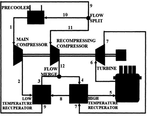
The input file contains pipe input data. CYCLES did not calculate pipe losses, and therefore did not have an input file for the pipes. Each pipe path is given a number, according to the pipe layout scheme shown in Figure 2.1. A description of the pipe paths is given in Table 2.2. Note that the reactor can also be an intermediate heat exchanger (IHX) when modeled as an indirect cycle.

PRECOOLERI

10 _LOW

SPLIT

Figure 2.1: Pipe Layout Scheme (Adapted from: Hejzlar et al., 2006) Table 2.2: Pipe Layout Scheme Description

Pipe Path Number Description

1 precooler to Main compressor

2 Main compressor and LTR

3 LTR to flow merge tee junction

5 LTR to flow merge tee junction

4 flow merge tee junction to HTR

5 HTR to IHX

6 IHX to turbine

7 turbine to HTR

8 HTR to LTR

9 LTR to flow split junction 10 flow split junction to precooler

11 flow split junction to recompressing compressor

The pipe data given in the HXdata. txt includes the diameter, cross-sectional area, length, form loss coefficient, and roughness. An abbreviated example of the pipe input data is given in Figure 2.2. A more detailed description of this pipe input data, including a description of the terms, as well as the other input data contained in HXdata. txt is provided in Section 3.2: Pipe and plena input data.

__··I__

0 0 0 0 000 0 k G r-I 0 0',I o 0 In o .-0 to_ooo 0 a NCNCl% r-I r-I N (h r-I Ro 0` $4 00 I I MN 0 0 Ooooo -rI 0 Eeooo tc m o 1 I% m_E-4 k * *r *rIkr 0 I-I-_0• 00 ;j O O O O U 0 A 0) v I I N M 00 * *4 I I I ooo 0000 I I I I 0000 o ooo O 5-Mr Pa N flu -# • *rI .rl P'S-S m_fu ·r4 0 In a p4 H

W-1

T-2.5

Output

CYCLES

The output for CYCLES is included in three files. One of the files, called res. txt, contains a summary of results, including overall and component efficiencies, work of the turbomachinery, heat transfer in the heat exchangers, and pressure drops in each of the components. The second file, cycres. txt, contains data for all the state points, including inlet and outlet temperatures, pressures, enthalpies, and entropies. The last file,

optimres. txt, contains the results of cycle optimization.

All of the data of the file res. txt is written on two lines, with the name of the output data on the first line, and the value on the data on the second line. In all, forty values are given across the two lines. The two lines spanned just over 360 columns. An abbreviated example of the first seven values of res .txt is:

pres-ra etal eta2 eta-net el-pow th-pow pumpwork...

2.600 50.787 50.770 50.696 304.691 599.942 541.684...

As shown, the descriptions of the variables above are abbreviations without units, but can be referenced in CyclesNew. doc.

The file cycres. txt contains five rows of numbers, with temperature points in the first column, pressure points in the second, enthalpy in the third, entropy in the fourth, and the fifth column is unused. The rows are grouped together by component: main compressor, recompressing compressor, turbine, low-temperature recuperator, and high-temperature recuperator. The data values are unlabeled, but can be referenced in CyclesNew. doc. An example of the output data in this file for the low-temperature recuperator is 60.9186 20000.0000 326.8039 0.0000 0.0000 156.3891 19991.1740 533.5467 0.0000 0.0000 0.0000 0.0000 0.0000 0.0000 0.0000 169.1683 7780.7524 605.2896 0.0000 0.0000 68.6519 7699.1980 477.1823 0.0000 0.0000 60.9186 7699.1980 464.0053 0.0000 0.0000

The first line contains values for the inlet on the cold side of the LTR, the second line has values for the outlet on the cold side, the third line is unused, the fourth has values of the inlet on the hot side, the fifth has values for ideal outlet conditions on the hot side, and the last line has values for the real outlet conditions.

CYCLES

II

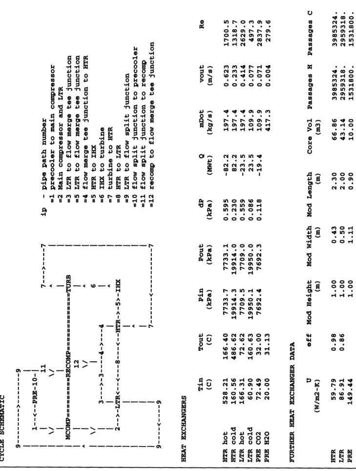
The output for CYCLES II combines important data from res. txt and cycres .txt into one file, output. txt. The output file is divided into five different sections: cycle schematic, heat exchangers, further heat exchanger data, turbomachinery, pipes, and overall cycle data. All numbers are explicitly labeled and include units (in the case where a number is dimensionless, no units are given). An example of the new output is shown in Figure 2.4.

Cycle Schematic - This section is provided as a visual to see where each of the components and pipes lies in relation to one other. Descriptions of the pipe path numbers, similar to those in Table 2.2, are given next to the schematic.

Heat Exchangers - This section provides important cycle state point parameters for the high-temperature recuperator, low-temperature recuperator, and precooler. Hot and cold side parameters are shown for each heat exchanger. Parameters include inlet and outlet temperatures and pressures, pressure drops, heat transfer rates, mass flow rates, outlet velocities, and Reynolds numbers. All values refer to the active length or core of the heat exchangers, which does NOT include the plena.

Further Heat Exchanger Data - This section provides further heat exchanger

parameters that pertain to the whole heat exchanger and not a particular side. Parameters include the overall heat transfer coefficient and effectiveness, as well as the module dimensions and the number of hot and cold channels. All values refer to the active length or core of the heat exchangers, which does NOT include the plena.

Turbomachinery - This section provides cycle state points parameters for the main

compressor, recompressing compressor, and the turbine. Parameters include inlet and outlet temperatures and pressures, pressure drops, power values, mass flow rates, efficiencies, and pressure ratios.

Pipes - This section provides important cycle state points for each of the pipes.

Parameters include inlet and outlet temperatures and pressures, pressure drops, and outlet velocities.

Overall Cycle - This section provides overall cycle data. Parameters include efficiency,

heat transfer rate in, heat transfer rate out, net power, pump power, minimum temperature difference in the heat exchangers, reactor pressure drop, overall flow rate, and fractional flow rate to the main compressor.

k 0 0 Tf 4), k kg 00 0l * .1 k 0 O *1 00 *) U r' gk S) 00+ o 0) 4)4)r 4,I 00k 14i *14 0 4)4) U i-I -I 4 mup 000U rlr4 0 4J'w k I In"~InC OF 0y-4C II II II II II II II II II II ri w-4 ri II II II III II A II In IIA II I II II P II I III I IIA V III I p4 '9 I I I II I tg I II I V II A III I II I V II I PS II EI IIA Pd I - ) -~ -t~~ 4)- o•-I-I r .14 ( .4 w~ (.4 In I I I I v I I I S.-I(.4 So ~On S0Oc)u

Figure 2.3a: Example of cycle output data contained in output.txt

In v 0 0 01-. (. 4) .-p4 WE'-4, 0 .1 0 (1)0r4 '9 I v-oov-I 000 000 Y.4Y-41-I', 0 I 0 I ri I I N A I I I I V I I I I I v.4-Iij C) C) II5P I~ -- - --- ~ br; S --- o ---- ~

O%0 B ' A.' d' A. ar M ' mnWMOO4W V4 CI M A Of 1 I W *****l0U ea wiO 0 -0 U o 0 W; O 1.00W C 0 0 t- '4 v M ri- M In I N ar rIm_I 0W owr* O •nI O)O1, o w-I Irn o W-M1 v M ,q ww MMMM • v • .n 0 Wt 0 w to '4 4w to Ln H4 C4 5_4' f --% 0 0 _o. rr NCM"Mwr-eMoCN '4'4'4

Figure 2.4b: Example of cycle output data contained in output.txt

00oo to En 0 0 0 0 0_o O O oa (4'40 C4 W; ; ,o I M PI JJ -Ow *16_Dii PIPI O q --. in rIU CO

E-1

I

I

2.6 Command window feedback

In CYCLES, when the program is executed successfully, the only feedback displayed to the command window is "recomp OK" after the convergence is complete. In an effort to show the user explicitly where the execution process is in the code, CYCLES II displays additional feedback to the command window. A typical execution of the program produces the following output to the command window:

reading file HXdata.txt...

make sure EX length is for zigzag channels

reading completed begin convergence 1 2 3 4 5 6 7 8 9 10 PRE converged

printing output to file output.txt... printing completed

The command window displays when the reading of the input files begins and ends, when the convergence algorithm begins and ends, and when the printing of the output begins and ends. The numbers 1-10 indicate the location of the execution process within the convergence algorithm.

2.7

Other simplifications

Optimization

CYCLES allows one to perform calculations on the recompression cycle one of two ways [Dostal, 2005]:

* Given the precise geometry of the heat exchangers, the code calculates single point efficiency, including the temperature and pressure drops across each component.

* Given a set total volume for the exchangers, the code optimizes the dimensions (length, width, and height) of the heat exchangers that will achieve the highest efficiency.

CYCLES II only performs the single point efficiency calculation and does not allow for optimization. This option was taken out for simplification. Furthermore, now that significant experience has been accumulated, a fairly narrow range can be pre-assigned for most independent variables.

Inter-cooling and re-heating

Both inter-cooling (using multiple compressors in series) and re-heating (using multiple turbines in series) are allowable in CYCLES. CYCLES allows these options in order to make the code more general, hence applicable to different S-C02 cycles. All calculations were performed on the recompression cycle. Also, since neither inter-cooling nor re-heating calculations is used in this cycle, these options are removed in CYCLES II for simplification.

2.8

Chapter summary

Many changes were made in CYCLES II in order to minimize the familiarization time, enhance the accuracy of the calculations, and reduce the complexity of the code:

* Instead of using common blocks to transfer global variables between subroutines, all global variables were placed in the module "modGlobalVariables".

* Variable names were changed to more easily recognizable names. For example, the value of the inlet temperature of the cold side of the low-temperature recuperator is stored in "ltr.TinCold" in CYCLES II, as opposed to "trl(1)" in CYCLES.

* Losses in both the pipes and the plena are taken into account in CYCLES II. * Straight or zigzag channel heat exchangers can be calculated

* Three different plate stacking patterns are allowed

* The input files for the heat exchangers and the pipes have been consolidated into one input file. The input file is commented so that the user knows the definition of each line of data, without having to reference a manual.

* Important output parameters are printed to one easily readable output file. The file is organized by component, and parameters are labeled with a description and units.

* The command window provides more feedback while the program executes to allow the user to know what is happening during the execution process.

* Optimization, inter-cooling and re-heating options have been removed from the code for simplification.

3 CODE DOCUMENTATION - FINAL VERSION

3.1 Introduction

CYCLES II is a modified version of the code CYCLES, which was written by Vaclav Dostal for his doctoral thesis at MIT in 2004. The code analyzes the steady-state thermodynamics of the S-C02 Brayton cycle. CYCLES II was modified specifically for the S-CO2 recompression Brayton cycle, which is shown schematically in Figure 2.1. All

changes that have been made to CYCLES are documented in Chapter 2. The purpose of this chapter is to provide a basic overview of the program for a new user to easily get acquainted with the code. A description of the input and output for the program is provided, and a flow chart is given to understand the algorithm logic.

3.2 Input

The input data for the program is written in the file HXdata. txt, which contains information on the overall cycle, heat exchangers, and pipes. At the end of the file, data for optimization purposes are also supplied. This section describes the input file and all its parameters.

The HXdata. txt file is broken up into six sections: "Main cycle input data", "HTR data", "LTR data", "PRE data", and "Pipe data". The actual titles of the sections are given in HXdata. txt, but the titles do not affect the calculations-they are read in and stored into a "dummy" variable that is never used. Each line, following the title of the section, contains one or more input parameters and a description of that input. The description always follows an exclamation mark. Anything written after the exclamation mark '!' is a comment and is not read in to the program. Where applicable, units are given in the description of the variable following the exclamation mark.

A Note on Turbomachinery Efficiency

When calculating the efficiency of turbomachinery components, it is important to know if the value indicates a total-to-total or total-to-static efficiency. Essentially, when a property is referred to as "total", such as total enthalpy, total temperature, or total pressure, it indicates that the velocity is taken into account. When a property is referred to as "static" it indicates that the velocity is not considered. Total conditions are typically used at the inlet of a turbine or compressor, but either total or static conditions can be used at the outlet [Cumpsty, 2004]. Either the difference in total-to-total enthalpies or the difference in total-to-static enthalpies can be used to calculate efficiency, which can lead to confusion if not explicitly stated which type is used. Dostal's code uses NIST

subroutines to calculate the conditions, which do not account for velocity (source). It is therefore best to consider the efficiency input values as a total-to-static efficiency.

To distinguish between the two efficiencies, first consider a control volume around a compressor. Under steady-state conditions and when assuming no heat transfer and no change in kinetic energy, the first law reduces to:

S= rh(k - h2) (3-1)

where W is the power required to run the compressor (W), rh is the mass flow rate (kg/s) of the working fluid, and hi and h2 are the specific enthalpies (J/kg) at the inlet and

outlet of the compressor, respectively. However, in some models, inlet and outlet velocities cannot be ignored. In the case where velocities are taken into account, the first law reduces to:

W = rh[(h - h -h (v - v2 ) / 2] (3-2)

where v indicates velocity (m/s). The enthalpy and velocity can be combined into one term, h,, which is the total (or stagnation) enthalpy:

ha = hI + v2 t/2 / 2 _1(3-3) h,2 = h2 + v/2

If the fluid as an ideal gas, then h is equal to cpT. Substituting this into the equations in (3-3) gives:

T = T+v2 / 2c

(3-4)

T,

=

T + v

/2c

where Tt is referred to as the total temperature. Combining equations 2), 3) and (3-4) gives:

W = hc, (T₁ - T2) (3-5)

To determine how the total enthalpies or total temperatures affect turbomachinery efficiency, we look at the efficiency of a compressor as an example, which is defined as:

Wideal

7c

=

where the subscript ideal refers to the case for an isentropic compressor and the subscript actual refers to the actual conditions. If total conditions are used at both the inlet and the outlet, then the efficiency is written as:

S=

(h

tt - ht2 actual

(3-7)

where ir, is the total-to-total efficiency, and all temperatures are denoted with a subscript 't' to indicate total values. If the total conditions are used at the inlet, but the static conditions are used at the outlet, then the efficiency changes to:

(3-8)

(hi1 - h2 ) actual

where St_, is the total-to-static efficiency and the temperature at the outlet is no longer total temperature but static temperature. Equation 3-8 is the convention adopted for

CYCLES II.

Main Cycle

Input

Data

An example of the input within the main cycle input data section is

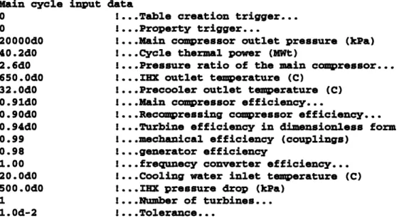
Main cycle input 0 0 2000040 40.240 2.6d0 650.040 32.040 0.91dO 0.90dO0 0.94d0 0.99 0.98 1.00 20.d00 500.040 1 1.04-2 data I.. I.. 1.. I.. o.. I.. I.o I.. I.. I..

.Table creation trigger... .Property trigger...

.Main compressor outlet pressure (kPa) .Cycle thermal power (MWt)

.Pressure ratio of the main compressor... .IHX outlet temperature (C)

.Precooler outlet temperature (C) .Main compressor efficiency...

.Recompressing compressor efficiency... .Turbine efficiency in dimensionless form .mechanical efficiency (couplings)

.generator efficiency

.frequnecy converter efficiency... .Cooling water inlet temperature (C) .IHX pressure drop (kPa)

.Number of turbines... .Tolerance...

As shown, for each line, the input parameter is given first, followed by a commented description. What follows is a more detailed description of each of the input parameters.

Table creation trigger - The table creation trigger is an integer, either '1' or '0', that

tables are created; if '0', old tables are used. If tables are created, the input file

createtables. txt must be used. An example createtables. txt input file

contains the following input:

200 ! .. .number of temperature points 200 !...number of pressure points 7000.0 1...table minimum pressure (kPa) 25000.0 !...table maximum pressure (kPa)

20.0 !... table minimum temperature (C)

650.0 !...table maximum temperature (C)

The above data, contained within the file createtables. txt, is only used if the table creation trigger is set to '1'.

Property trigger - The property trigger is an integer, either '1' or '0', that determines

whether to use property tables or NIST 12 pure fluid property subroutines. If '1', subroutines are used; if '0', tables are used. The NIST 12 subroutines are more accurate, but take much longer to converge to a solution (on the order of hours). The tables are less accurate, but take much less time to converge to a solution (on the order of seconds).

Main compressor outlet pressure - This is both the pressure at the outlet of the main

compressor as well as the maximum cycle pressure in kPa. The user should be cautious in changing this value because the pressure ratio of the main compressor should be changed in conjunction with it.

Cycle thermal power - The cycle thermal power, given in MWt, is the heat transfer rate

into the cycle through the intermediate heat exchanger (IHX). The fixed cycle thermal power is used to calculate the mass flow rate by the formula:

rh = , (3-9)

Ah

where

Qi,

Pressure ratio of the main compressor - The pressure ratio of the main compressor is

the ratio of the pressure at the outlet of the compressor to the pressure at the inlet of the compressor and is a dimensionless quantity:

mm Pout ,mcomp (3-10)

in,mcomp

where rmcomp is the pressure ratio of the main compressor, Pou,,tomp is the pressure at the

outlet of the main compressor (kPa), and Pin,mcomp is the pressure at the inlet of the main

IHX outlet temperature - This is both the intermediate heat exchanger outlet temperature (°C) and the maximum cycle temperature.

Precooler outlet temperature - This is the precooler outlet temperature (°C) of the

working fluid, CO2.

Main compressor efficiency - The main compressor efficiency is the dimensionless quantity used to calculate the power required to run the main compressor by the formula:

- hm (hn - hut'i (3-11)

mcomp 103· "7 mcomp

where Wlcom, is the power required to run the main compressor (MW), rhmcomp is the mass

flow rate through the main compressor (kg/s), hin is the specific enthalpy at the inlet of the main compressor (kJ/kg), hour., is the ideal specific enthalpy at the outlet of the main

compressor (kJ/kg), and rlmcomp is the main compressor efficiency (on a total-to-static

basis).

Recompressing compressor efficiency - The recompressing compressor efficiency is

the dimensionless quantity used to calculate the power required to run the recompressing compressor by a formula similar to that given in equation (3-11), except that each of the quantities refers to that of the recompressing compressor.

Turbine efficiency - The turbine efficiency is the dimensionless quantity used to

calculate the power supplied by the turbine by the formula:

W

_*u

_hrb

_'

(h,

hout,;)

_(3-12)

103

where W,rb is the power supplied by the turbine (MW), rhrb is the mass flow rate

through the turbine (kg/s), hi, is the specific enthalpy at the inlet of the turbine (kJ/kg),

hou,.' is the specific enthalpy at the outlet of the turbine (kJ/kg), and 7turb is the turbine

efficiency (on a total-to-static basis).

Mechanical efficiency (couplings) - The mechanical efficiency, which accounts for the

friction and rubbing of the gears, affects the calculation of the net power of the system by the formula:

net rb * mech mp ) +mc ec (3-13)

where Wet,,, is the net power (MW), 7_{,mech is the mechanical efficiency, and the power}

subscripts "turb", "mcomp", "recomp", and "pump" refer to the turbine, main compressor, recompressing compressor, and pump, respectively.

Generator efficiency and frequency converter efficiency - These two efficiencies are combined to yield the electric efficiency. The generator efficiency accounts for how well mechanical power is converted into electrical power, and frequency converter efficiency accounts for how well AC is converted into (and/or from) DC. The electrical efficiency affects the calculation of the net cycle efficiency by the following calculations:

Wnet

•net = 1elec ₍

Qin (3-14)

7

elec = 'gen • )fcon

where rlne, is the net efficiency, and the subscripts "elec", "gen", and "fcon" stand for

electrical, generator, and frequency converter efficiency, respectively.

Cooling water inlet temperature - This is the inlet temperature of the cooling water in the precooler and the minimum cycle temperature in 'C.

IHX pressure drop - The IHX (or reactor, for a direct cycle) pressure drop is the difference between the pressure at the inlet of the IHX and the pressure at the outlet of the IHX in kPa (a positive quantity):

dPIHX = n,HX Pout,IHX (3-15)

where dPHx is the IHX pressure drop (kPa), 4PnWx is the IHX inlet pressure (kPa), and

Pout,rIx is the IHX outlet pressure (kPa). The IHX is not modeled in CYCLES II, but

input as a fixed pressure drop.

Tolerance - The tolerance is used to determine when to stop the convergence algorithm. A lower value ensures a more precise solution, while a higher value obtains a converged solution more quickly. At the end of the convergence loop, the fractional pressure drop of a component is compared to the tolerance. The fractional pressure drop of a component is calculated by the formula:

dPn - dPn-I

Fractional pressure drop = (3-16)

dJP

where dP, is the pressure drop of a particular component (LTR, HTR, or PRE) on the nth convergence loop, and dP,__{1 is the pressure drop of the same component on the previous} convergence loop. As the convergence algorithm begins to reach a more accurate

solution, the value of the fractional pressure drop decreases. The convergence algorithm will exit when it reaches a value that is less than the tolerance. A typical value for the tolerance is 0.01.

HTR data

An example of the input within the HTR data section is

HTR data

htr !...HX type

strlhlc ! ... .Channel type...

0.002 !...hot channel diameter (m)

0.002 !...cold channel diameter (m)

0.0015 !...hot plate thickness (m)

0.0015 !...cold plate thickness (m)

1.0 !...module height (m)

0.434783 !... module width (m)

2.3 !...module length (m)

66.86 !...heat exchanger volume (m3)

25.0 !...plate thermal conductivity (W/m-K)

40.0 !...number of axial nodes...

0.005 !...precision

100.0 !...initial step

1.3 !...initial step adjustment

Similar to the main cycle input data, for each line, the input parameter is given first, followed by a commented description. What follows is a more detailed description of each of the input parameters.

HX type - The heat exchanger type is a three character string that indicates the type of heat exchanger ('htr' for high-temperature recuperator, 'Itr' for low-temperature recuperator, and 'pre' for precooler).

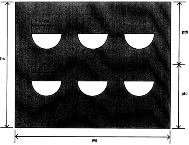
Channel type - The channel type is a seven character string that indicates the type of channels used in the heat exchanger and the stacking pattern for the plates. If the first three letters are "str", then the channels are straight; if the first three letters are "zig", then the channels are of the zigzag type. The last four letters indicate the stacking pattern. The last four letters can either be "lhlc" a one-hot, one-cold alternating stacking pattern, "lh2c" for a one-hot, two-cold stacking pattern, or "2hlc" for a two-hot, one-cold stacking pattern.

hs

N

Figure 3.1: Heat exchanger profile

Hot channel diameter - This is the diameter Dh in meters of the semicircular-shaped hot channels shown in Figure 3.1.

Cold channel diameter - This is the diameter Dc in meters of the semicircular-shaped cold channels shown in Figure 3.1.

Hot plate thickness - This is the thickness pth in meters of the hot plates as shown in Figure 3.1.

Cold plate thickness - This is the thickness ptc in meters of the cold plates as shown in Figure 3.1.

OP

L

.I

Figure 3.2: Dimensions of heat exchanger module

Module height - _{This is the height hs in meters of one heat exchanger module as shown}

in both Figure 3.1 and Figure 3.2.

Module width - This is the width ws in meters of one heat exchanger module as shown in both Figure 3.1 and Figure 3.2.

Module length - _{This is the length Is in meters of one heat exchanger module as shown}

in Figure 3.1.

Heat exchanger volume - _{This is the total volume of the heat exchanger core in m}3

.

Each module has a volume (length x width x height) of 1 m3_{, so the recuperator volume}

is also the total number of modules used in the calculation.

Plate thermal conductivity - _{This is the thermal conductivity of the plate in (W/m-K).}

Number of axial nodes - _{This is the number of axial nodes used to calculate the thermal}

performance of the heat exchanger. The heat exchanger calculations use a convergence algorithm whereby the heat exchanger is broken up into many different axial nodes and the heat transfer is analyzed iteratively until a solution is converged.

Precision - This value is used in the convergence loop within the heat exchanger subroutines to determine how precise the calculations need to be before the convergence loop ends. A typical value is 0.005.

Initial step - This is the first value used as an increment to iterate a solution for the recuperator subroutine. A typical value for a 300 MWe cycle is 100. This value needs to be scaled with power. Thus, for a 100 MWe cycle, this value should be reduced to 0.333. Initial step adjustment - This value is used to change the value of the incremental step each time convergence is not obtained. A typical value is 1.3 and is independent of power values.

LTR data

An example of the input within the LTR data section is

LTR data

htr I... HX type

strlhlc I... Channel type...

0.002 !...hot channel diameter (m)

0.002 !...cold channel diameter (m)

0.0015 !...hot plate thickness (m)

0.0015 i...cold plate thickness (m)

1.0 I...module height (m)

0.5000 1...module width (m)

2.0 I...module length (m)

43.14 ! ...heat exchanger volume (m3)

25.0 !...plate thermal conductivity (W/m-K)

40.0 !...number of axial nodes...

0.005d0 I...precision

100.Od0 !...initial step

1.3d0

l...

As shown, the input data for the low-temperature recuperator has the same number and type of parameters as the high-temperature recuperator. For a detailed description of each of the input parameters, refer to the previous section on "HTR data".

PRE data

An example of the input within the PRE data section is

PRE data

pre I .. .HX type

strlhlc I ... Channel type...

0.002 I...hot channel diameter (m)

0.002 _{!...cold channel diameter (m)}

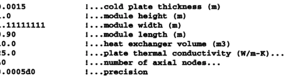
0.0015 1.0 1.11111111 0.90 10.0 25.0 40 0.0005d0

!...cold plate thickness (m) I...module height (m)

I .. .module width (m) I...module length (m)

!... heat exchanger volume (m3)

!...plate thermal conductivity (W/m-K) ...

!...number of axial nodes... I...precision

As shown, the input data for the precooler has almost the same number and type of parameters as the data for both the high-temperature recuperator and the low-temperature recuperator. The only difference is that the precooler data lacks two parameters: initial step and initial step adjustment. For a detailed description of each of the input parameters, refer to the previous section on "HTR data".

Pipe and plena data

The pipe data includes the information about the geometry and physical characteristics of the pipes, as well as that for the various plena. An abbreviated example of the input within the Pipe data section is given in Figure 3.3. The data is divided up into pipe paths, (labeled "precooler to main compressor", "main compressor to LTR", etc.) where each pipe path is numbered in the cycle schematic in Figure 2.1. The pipe paths contain different sections, where each section is made up of one or more identical pipes or plena. When multiple pipes or plena are given in a section, it indicates that they are parallel. A description of each of the sections within the pipe paths is provided as a comment in the right-most column. The data is sorted into columns, and the titles of the columns indicate the variable type.

pipe path sectior

variables

Pipe

)

.a.t

IP Nsec NpZipe Dpipe(ip) ...

precooler to

pipe path name

main compressor 1 4 72 0.1576 .1 37038 0.0030 *1 4 0.2400 61 2 0.500 main compressor to LTR 2 4 2 0.500 2 4 0.3048 2 12 0.3048 2 72 0.1151 LTR to merge T junction

... !precooler outlet plenum LP

... Iprecooler outlets LP

... lannular outlet - vessel

... Ipipe to main compressor

!distributing pipes

... ILTR inlet side plen

... !LTR inlet dist. plez

section descriptions

um HP

na HP

A description of the variables used to store the data in the pipe data section is given in Table 3.1.

Table 3.1: Description of variables used in the "Pipe data" section of HXdata.txt

Variables Description

ip pipe path number

NSec (ip) number of pipe sections with different flow areas (in series) for each path ip Npipe (j ip) number of parallel passages in section j of path ip

Dpipe (j, ip) hydraulic diameter for section j of path ip (m) Apipe (j, ip) cross sectional area for section j of path ip (m2) ELpipe (j,ip) pipe length for section j of path ip (m)

xsipipe (j, ip) form loss coefficient for section j of path ip (dimensionless) roughpipe (j,ip) pipe roughness for section j of path ip (m)

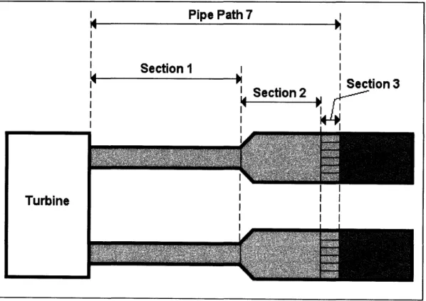
The pipe layout scheme given in Figure 2.1 can be misleading, since a pipe path can include multiple pipes and plena. For example, for the pipe path from the turbine to the HTR, it could consist of two turbine exhaust pipes in parallel, followed by distributing pipes, then thousands of inlet channels, and finally, fifty or more inlet plena that lead into the passages of the HTR core. To understand the basics of the pipe and plena input data in the input file, a simplified example is given in Figure 3.4 that shows a pipe path that runs from the turbine to two high-temperature recuperators.1

Figure 3.4: Pipe and plena input example

The pipe path is divided into three sections: section 1 contains two pipes in parallel, each with a diameter 0.3 m, section 2 contains two distribution pipes of 0.6 m, and section 3 contains two sets of 6 plena, each with a diameter of 0.1 m, that lead to the HTR core. The input data given in the input file for pipe path 7 is given in Figure 3.5.

Pipe data

IP Nsec Npipe Dpipe(ip) Apipe(ip) ELpipe(ip) xsi_pipe(ip) rough_pipe

(m) (m2) (m) (m)

turbine to HTR

7 3 2 0.3 0.07069 2.00 0.60 1.0E-04

7 2 0.6 0.28274 1.00 1.90 1.0E-04

7 12 0.1 0.00785 0.15 1.20 1.0E-04

Figure 3.5: Pipe and plena input data example

The pipe path name is "turbine to HTR", and the pipe path number (ip) is 7, as shown for each of the sections in the left-most column of numbers. The second column contains one number which indicates the number of sections (Nsec). The third column gives the diameter of each of the pipes or plena in the pipe paths sections. Notice that in the third section, the total number of plena equals 12 and not 6, since all plena in parallel are counted. For non-circular pipes, this value would be a hydraulic diameter. The cross sectional area is listed in the fourth column. For this example, the pipes were made circular, so the cross sectional area is simply D2 r / 4. The length of the sections is given under "ELpipe". The values "xsi_pipe" and "rough_pipe" are simply the form loss coefficients and roughness for each section.

3.3

Output

The output data for the program is written in the file output. txt, which contains data for heat exchangers, turbomachinery, pipes, and the overall cycle. Also included is a cycle schematic for reference. _{This section describes the output file and all its} parameters.

The output. txt file is broken up into five sections: "Cycle schematic", "Heat exchangers", "Further heat exchanger data", "Turbomachinery", "Pipes", and "Overall cycle". An example of all the data contained in the output file is given in Figure 2.4.

Cycle Schematic

This section provides a simple cycle schematic with all the components and pipe path numbers. The arrows along the pipe paths are provided to show the direction of mass flow. The connection between the main compressor, recompressing compressor, and the turbine represents the shaft. Descriptions of the pipe path numbers are given next to the schematic. A list of the terms used in this section and a description for each is given in Table 3.2.

Table 3.2: Description of terms used in the "Cycle Schematic" section of outputtxt

Terms Description

HTR high-temperature recuperator

LTR low-temperature recuperator

PRE precooler

MCOMP main compressor

RECOMP recompressing compressor

TURRB turbine

IHX intermediate heat exchanger

merge junction intersection of pipes 3, 4, and 12 split junction intersection of pipes 9, 10, and 11

Heat Exchangers

This section provides important cycle state point parameters for the high-temperature recuperator, low-temperature recuperator, and precooler. Hot and cold side parameters are shown for each heat exchanger. A list of the terms used in this section and a description of each is given in Table 3.3. All values refer to the active length or core of the heat exchangers, which do NOT include the plena.

Table 3.3: Description of terms used in the "Heat Exchangers" section of outputtxt

Terms Description

HTR hot hot side of high-temperature recuperator

HTR cold cold side of high-temperature recuperator

LTR hot hot side of low-temperature recuperator

LTR cold cold side of low-temperature recuperator

PRE C02 CO2 side of precooler

PRE H20 cooling water side of PRE

Tin (C) inlet temperature in 0C

Tout (C) outlet temperature in oC

Pin (kPa) inlet pressure in kPa

Pout (kPa) outlet pressure in kPa

dP (kPa) inlet pressure minus outlet pressure in kPa

Q (MWt) heat transfer rate in MWt (positive is heat in, negative is heat out)

mdot (kg/s) mass flow rate in kg/s

vout (m/s) outlet velocity in m/s

Re Reynolds number (dimensionless quantity)

Qstrewa = i -(hou, - hn ). 10-3

where Qstream is the heat transfer rate (MWt) for either the hot or cold stream, rt is the

mass flow rate (kg/s) for that stream, and ho,t and hin are the outlet and inlet specific

enthalpies (kJ/kg) for that stream, respectively. The mass flow rate of each stream is determined by the total mass flow rate of the system and, for the LTR, the fraction of the flow rate that splits to the main compressor. The outlet velocity of each stream in the heat exchangers is calculated as follows:

passage

Vout ,stream "-- (3-18)

where voW,stream is the outlet velocity (kg/s) for either the hot or cold stream, rihsage is the mass flow rate of the fluid per passage for that stream, p is the density of the fluid

(kg/m3_{) at the outlet for that stream, and Aassge is the passage cross sectional area (m2).}

The Reynolds number of each stream in the heat exchangers is calculated as follows:

d h mhpassage

Re stream dh ssage (3-19)

# "Apassage

where Restream _{is the Reynold's number (dimensionless) for either the hot or cold stream,}

dh is the hydraulic diameter of a passage (m), and

u

Further Heat Exchanger Data

This section provides the overall heat transfer coefficient and effectiveness for each heat exchanger, as well as the module dimensions and the number of hot and cold channels. All parameters refer to the heat exchangers as a whole. A list of the terms used in this section and a description of each is given in Table 3.4.

Table 3.4: Description of terms used in the "Further Heat Exchanger Data" section

Terms Description

HTR high-temperature recuperator

LTR low-temperature recuperator

PRE precooler

U (W/m2-K) _{overall heat transfer coefficient in W/(m}2_-K)

eff effectiveness

Mod Height (m) module height in meters Mod Width (m) module width in meters Mod Length (m) module length in meters

Core vol (m3) core volume in m

Passages H total number of hot passages

Passages C total number of cold passages