HAL Id: hal-01831897
https://hal.archives-ouvertes.fr/hal-01831897
Submitted on 6 Jul 2018
HAL is a multi-disciplinary open access archive for the deposit and dissemination of sci-entific research documents, whether they are pub-lished or not. The documents may come from teaching and research institutions in France or abroad, or from public or private research centers.
L’archive ouverte pluridisciplinaire HAL, est destinée au dépôt et à la diffusion de documents scientifiques de niveau recherche, publiés ou non, émanant des établissements d’enseignement et de recherche français ou étrangers, des laboratoires publics ou privés.
Integral Shape Averaging applied to delayed windows of
the same signal
Hervé Rix
To cite this version:
Hervé Rix. Integral Shape Averaging applied to delayed windows of the same signal. [Research Report] Laboratoire I3S / UNS; UMR 7271 UNS/CNRS member of UCA. 2018. �hal-01831897�
1
Research Report
Integral Shape Averaging applied to delayed windows of the same signal. Hervé Rix
Lab. I3S, UMR 7271 UNS/CNRS, SIS Team Université Nice- Sophia Antipolis member of UCA
ABSTRACT
Integral Shape Averaging (ISA) is a technique for averaging a series of positive signals using their normalized integrals. In case of equal shape signals, ISA gives an estimation of this shape with an increased SNR due to integration. A new application of ISA is presented here: from only one recording of a positive signal embedded in noise, applying ISA to a series of delayed windows containing the signal can give a good estimation of this signal. Simulation results are given on a double and then a triple Gaussian embedded in white zero mean noise, with different SNRs.
INTRODUCTION
The estimation of a signal embedded in another one, considered as noise, with a low signal to noise ratio (SNR), and present in a series of realizations is commonly made by the classical signal averaging method (or synchronous averaging). In the biomedical domain the main applications are in High Resolution Electrocardiography (HR ECG) for the detection and estimation of late potentials (LP) embedded in Electromyography (EMG) signal, and for Evoked Potentials (EP) embedded in EEG. In the first application the alignment for averaging is synchronized on the QRS complex, commonly the R wave. In the second one, the trials are aligned using the stimulus time. This averaging technique is optimal when all the averaged signals are the same shape with a perfect alignment, i.e. no jitter, and also no time scaling factor. In fact, due to physiology, random time shift and time scale fluctuations are often present which modify the common shape as detailed in [1]. If shape equality of two signals is the invariance through increasing affine transformations, the averaged signal, using Integral Shape Averaging (ISA), of a set of equal shape positive signals is the same shape with the mean position and the mean scale factor [1], [2].
In case of poor SNR an option is to increase the number or averaged signals. This is generally possible when the stimulus is repetitive, e.g.in auditory EPs. But if we are interested in cognitive EPs, like N400 wave emitted by the brain when a semantic incongruity is
detected, the stimulus must be changed at each trial. For further application to this situation the following method is proposed which artificially multiplies the number of averaged signals. The theory is explained in the next section, and then a simulation study with a double and then a triple Gaussian embedded in white noise is presented with different SNRs. The aim of
2
the paper is to present a new method improving the SNR on a single realization of a noisy signal, with the only information that the embedded signal is positive. Applications to practical situations like cognitive EP estimation are foreseen in a further work.
THEORY
1. Hypotheses
Let s(t) and v(t) be two positive signals, with finite supports, they will be said the same shape if and only if they are linked by equation (1) or its equivalent form (2).
0 0 ) ) (( . ) (t ks td a C k a v (1) k C C k k C d at v k t s( ) '. ( ) ' '1/ ' / (2)
Practically the offset C is assumed to be zero after subtracting a linear base line.
The data are a series of N positive equal shape signals embedded in zero mean noise, with random fluctuations of their time occurrences, their heights and their widths, as defined in (3):
N i t n a d t s k t si( ) i (( i)/ i) i( ) 1 (3)
In this equation ki , di and ai are realizations of independent random variables K, D and A, and
ni(t) is a sequence of the random zero mean noise n(t). In fact, for computation we have to
deal with the discrete form of (3) where the variable t is sampled in M equidistant values tj,
with step h, j=1 to M, leading to system (4):
M j N i t n a d t s k t si( j) i (( j i)/ i) i( j) 1 1 (4)
Every signal si(t) is assumed to have a finite support, each support being boarded by two
intervals with only noise, and included in a larger time interval [0,T]. Since we cannot know the exact support of the signal in every single trial, we take a larger interval [T1, T2],
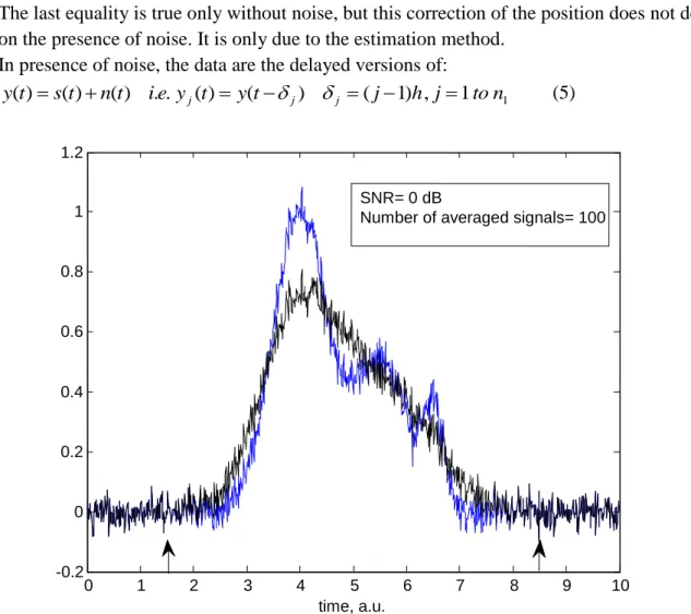
practically the union of all the supports, in estimating the support of the classical average. As shown in Fig.1, the signal support is assumed to be included in interval [T1, T2], which is
included in the larger interval [0, T], where T1=1.5, T2=8.5 (indicated by the arrows on the time axis) and T= 10. With our previous notations, we have:
Mh
T and let put: T1 n1h T2 n2h
2. Definition of the delayed windows
For a given trial, ISA signal is computed over the (n1+1) windows [0, T2], [h, T2+h]… [T1,
T2+T1] containing the same noisy signal, with different sequences of noise before and after
the signal. This ISA signal obtained on delayed versions of the same signal will be called ISAD. On Fig.1 the window sequence goes from [0, 8.5] to [1.5, 10]. Since we have only one trial, the index of s will be omitted. Without noise, all these windows move from left to right around the same signal s(t). For ISA it’s the same as moving the signal from right to left on a time distance T1. So the ISAD signal is this signal centered at the mean position i.e. at
3
T1/2. To get the good estimation we need to translate the ISA signal from left to right
according to T1/2. In other words, if w(t) is the ISAD signal, without noise, we have:
)) 2 / ( ( ) (t s t T1
w , and the estimate of s(t) is: ) ( )) 2 / ( ( ) (t wt T1 s t s
The last equality is true only without noise, but this correction of the position does not depend on the presence of noise. It is only due to the estimation method.
In presence of noise, the data are the delayed versions of:
1 1 , ) 1 ( ) ( ) ( . . ) ( ) ( ) (t s t nt ie y t yt j h j ton y j j j (5)
Fig. 1 Signal averaging with and without jitter or time scale fluctuations
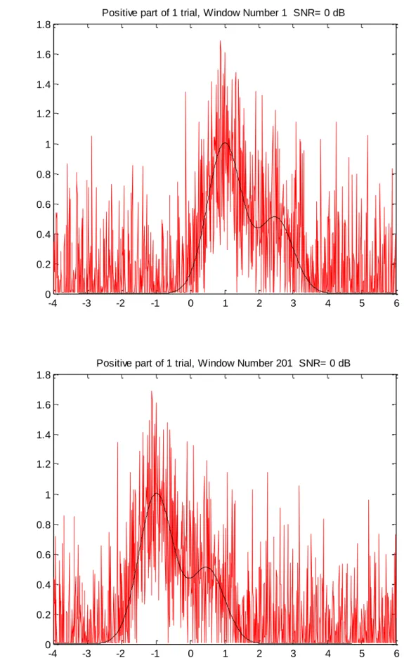
In fact since ISA must be applied to positive signals, it is applied to the positive part z(t) of y(t) defined in (6) : elsewhere zero and t y if t y t z( ) ( ) ( )0 (6)
In Fig. 2, an example of the first and the final window is shown, for signal z(t) defined in (6).
0 1 2 3 4 5 6 7 8 9 10 -0.2 0 0.2 0.4 0.6 0.8 1 1.2 time, a.u. SNR= 0 dB
4 -4 -3 -2 -1 0 1 2 3 4 5 6 0 0.2 0.4 0.6 0.8 1 1.2 1.4 1.6 1.8
Positive part of 1 trial, Window Number 1 SNR= 0 dB
-4 -3 -2 -1 0 1 2 3 4 5 6 0 0.2 0.4 0.6 0.8 1 1.2 1.4 1.6 1.8
Positive part of 1 trial, Window Number 201 SNR= 0 dB
5
SIMULATION STUDY WITH WHITE NOISE
The simulation study was made on two signal models: y2 and y3 representing the sum of two
Gaussians (7) and three Gaussians (8) respectively.
) ) 5 . 0 5 . 1 ( 5 . 0 exp( 5 . 0 ) ) 5 . 0 ( 5 . 0 exp( ) ( 2 2 2 t t t y (7) ) ) 2 . 0 5 . 2 ( 5 . 0 exp( 3 . 0 ) ( ) ( 2 2 3 y t t t y (8)
Then white noise sequences were added to these models for given signal to noise ratios (SNR). The averaging of such noisy signals gives an idea of SNR improvement in the ideal case, i.e. without jitter or scale factor fluctuations (Fig.1, blue curve). Since we are dealing with such possible fluctuations of the position and the width of averaged signals, a random delay and a random scale factor were introduced. Their values were chosen in order to obtain an averaged signal with only one maximum, for both the sums of two and three Gaussians. An example of the filtering effect of averaging in this case can be seen on Fig.1.
-4 -3 -2 -1 0 1 2 3 4 5 6 -0.1 0 0.1 0.2 0.3 0.4 0.5 0.6 0.7 0.8
Average of 200 trials with jitter and scale fluctuations
6
Fig. 4 Comparison of classical and ISA averaging, without noise
-4 -3 -2 -1 0 1 2 3 4 5 6 0 0.2 0.4 0.6 0.8 1 1.2 1.4
Averaging without noise, 2 peak model
b: The 2 peak model
g: Classical averaging of 200 trials r: ISA of 200 trials -4 -3 -2 -1 0 1 2 3 4 5 6 0 0.2 0.4 0.6 0.8 1 1.2 1.4
Averaging without noise, 3 peak model
b: The 3 peak model
g: Classical averaging of 200 trials r: ISA of 200 trials
7 -4 -3 -2 -1 0 1 2 3 4 5 6 0 0.2 0.4 0.6 0.8 1 1.2 1.4 1.6
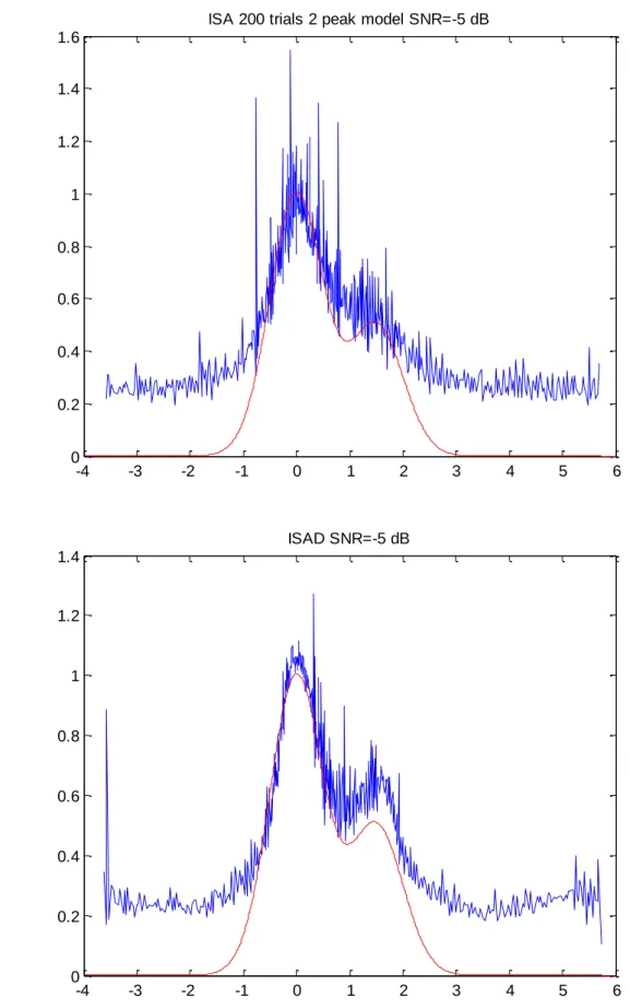
ISA 200 trials 2 peak model SNR=-5 dB
-4 -3 -2 -1 0 1 2 3 4 5 6 0 0.2 0.4 0.6 0.8 1 1.2 1.4 ISAD SNR=-5 dB
8 -4 -3 -2 -1 0 1 2 3 4 5 6 0.1 0.2 0.3 0.4 0.5 0.6 0.7 0.8 0.9 1 1.1
ISA of 200 signals, 3 peak model, SNR=0 dB
-4 -3 -2 -1 0 1 2 3 4 5 6 0.1 0.2 0.3 0.4 0.5 0.6 0.7 0.8 0.9 1 1.1
9 -4 -3 -2 -1 0 1 2 3 4 5 6 0 0.2 0.4 0.6 0.8 1 1.2 1.4
ISAD 1 trial (IK=5) 2 peak model, SNR= 0 dB
-4 -3 -2 -1 0 1 2 3 4 5 6 0 0.2 0.4 0.6 0.8 1 1.2 1.4
10 -4 -3 -2 -1 0 1 2 3 4 5 6 0 0.2 0.4 0.6 0.8 1 1.2 1.4
ISAD 1 trial (IK=15) 3 peak model, SNR= 0 dB
Fig. 6 Examples of ISA and ISAD for the 2 peak and 3 peak models, SNR= 0 dB
In these precedent examples we can see that ISAD gives on one trial and 200 windows a better estimation than ISA on 200 trials. In fact we have about 20 realizations to make 20 estimations with ISAD. This number is the maximum allowed if we want to make a classical average with different stimuli. In our case we observed variability in shape estimation by ISAD: but we can choose the” best one” or one of the best ones, computing the ISA signal of these 20 ISAD signals, the shape difference (using DFM) of each ISAD to this class centre, and also their mutual shape differences for outliers elimination.
11 -4 -3 -2 -1 0 1 2 3 4 5 6 -0.2 0 0.2 0.4 0.6 0.8 1 1.2 2 peak model SNR= 0 dB
r: Ideal synchronous averaging b: ISAD 1 trial, 200 windows k: Affine transformation of b to eliminate the offset.
In this example, we obtain from only one trial, without any information on the embedded signal except its positivity, practically the best estimation we could expect by the classical averaging of 200 trials in case of perfect alignment and no scale fluctuation!
REFERENCES
[1] - RIX H., MESTE O., MUHAMMAD W.
« Averaging Signals with Random Time Shift and Time Scale Fluctuations », Methods of Information in Medicine 2004, Vol. 43, pp.13-16.
[2]- BOUDAOUD S., RIX H., MESTE O.
« Integral Shape Averaging and Structural Average Estimation: A Comparative Study ». IEEE Trans. Signal Processing, 2005, Vol. 53, No. 10, pp. 3644-3650. hal-00356065