HAL Id: hal-03156583
https://hal.archives-ouvertes.fr/hal-03156583
Submitted on 11 Mar 2021
HAL is a multi-disciplinary open access
archive for the deposit and dissemination of
sci-entific research documents, whether they are
pub-lished or not. The documents may come from
teaching and research institutions in France or
abroad, or from public or private research centers.
L’archive ouverte pluridisciplinaire HAL, est
destinée au dépôt et à la diffusion de documents
scientifiques de niveau recherche, publiés ou non,
émanant des établissements d’enseignement et de
recherche français ou étrangers, des laboratoires
publics ou privés.
Investigating SEM-contour to CD-SEM matching
François Weisbuch, Jirka Schatz, Sylvio Mattick, Nivea Schuch, Thiago
Figueiro, Patrick Schiavone
To cite this version:
François Weisbuch, Jirka Schatz, Sylvio Mattick, Nivea Schuch, Thiago Figueiro, et al.. Investigating
SEM-contour to CD-SEM matching. SPIE Advanced Lithography, Feb 2021, Online Only, France.
�10.1117/12.2583715�. �hal-03156583�
Investigating SEM-contour to CD-SEM matching
Francois Weisbuch
a, Jirka Schatz
a, Sylvio Mattick
a, Nivea Schuch
b, Thiago Figueiro
b, Patrick Schiavone
b,c aGLOBALFOUNDRIES, Wilschdorfer Landstraße 101, 01109, Dresden, GERMANY
b
Aselta Nanographics, 4, place Robert Schuman, 38000 Grenoble, FRANCE
c
Univ. Grenoble Alpes, CNRS, CEA/LETI-Minatec, Grenoble INP, LTM, F-38054 Grenoble-FRANCE
ABSTRACT
Background: The control and the characterization of semiconductor very fine devices on a wafer are commonly
performed by mean of a scanning electron microscope (SEM) to derive a critical dimension (CD) from a pair of parallel edges extracted from the images. However, this approach is often not very reliable when dealing with complex 2D patterns. An alternative is to use SEM contour technique to extract all the edges of the image. This method is more versatile and robust but before being implemented in a manufacturing environment, it must demonstrate that it can be matched well with traditional CD-SEM.
Aim: The objective of this work is to present a method to evaluate and optimize the CD matching between a reference
standard SEM-CD and SEM-Contours.
Approach: After describing the metric used to assess the matching performance, we propose to screen some important
influent parameters to give an evaluation of the best matching that we achieved with our experimental data.
Results: After optimizing the matching calibration parameters and optimizing the selection of the best anchor pattern for
the matching we could achieve a 3s-Total Measurement Uncertainty of 0.8 nm and 3.2 nm for 1D and 2D patterns.
Conclusions: We established a method to achieve good matching performance that should facilitate the introduction of
SEM contour in a manufacturing environment.
Keywords: SEM, contour, critical dimension, matching, metrology, contour metrology 1. INTRODUCTION
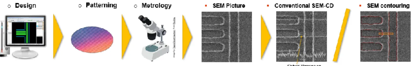
The characterization and the control of the dimensions of semiconductor very fine devices are commonly performed by mean of a scanning electron microscope (SEM) able to generate high-resolution top-down grayscale images. The standard approach is to process only a portion of the image restricted to a measurement window to derive a critical dimension (CD) from a pair of extracted parallel edges. However, when dealing with complex 2D patterns, the size of the measurement window can be very small which often decreases the reliability of the measurements unless spending a lot of effort to set up a robust metrology recipe. The increase of complexity and the diversification of the semi-conductor applications require always more such patterns to be precisely measured not only for engineering purposes but also in the context of manufacturing metrology.
Fig. 1: Conventional SEM-CD vs SEM-contour flow.
An alternative approach has emerged, which consists in taking into account all the edge information contained in the image by extracting SEM contours as shown in Fig. 1. Capturing more edge information often implies that fewer SEM images are needed and so the metrology cycle time can be greatly improved [1]. By construction, SEM contours are capable of characterizing very complex 2D-shapes without the restriction of having parallel edge pairs. Besides, SEM
contour extraction generates polygons to describe a pattern instead of a single CD number. This abstraction opens the door to new applications. By describing completely any pattern given by a SEM image, SEM contours are very valuable for OPC compact model [2, 3, 4, 5] or rigorous model [6] calibrations because they improve the design space coverage. SEM-contours are a very rich data source for any machine learning application [7, 8]. In addition, SEM-contours from different images can be combined to characterize the evolution of a pattern upon different process conditions, like micro-lens reflow [9], litho-etch bias [10] or perform in-situ overlay between patterns measured on different layers during the manufacturing [11]. Another advantage is that the contours represented with polygons can be merged with design. Hence, the nature of the contours offers new metrics for the metrology like Edge Placement Error [11], the measure of a pattern shift [12] or even characterization of pattern topography by considering contours measured at different heights in a material [13].
Even more fascinating applications are to come that stress the necessity to address the many challenges of handling SEM-contours, like edge extraction complexity with noisy or multi-pattern images, like contour post processing to align, clean and average contours, like bringing new concepts for pattern sampling and dedicated test pattern generation in the context of model calibration…An additional challenge, that we propose to discuss specifically in this work, is the question of the matching of SEM-contour to standard SEM-CD [10, 14]. The demonstration of the compatibility of SEM-contour with a reference SEM-CD appears to be a pre-requisite to establish SEM-contour as a reliable and mature alternative metrology method that can be adopted in a manufacturing environment.
Fig. 2 Standard SEM-CD vs SEM-Contour matching.
The objective of this work is to present a method to evaluate and optimize the CD matching (see Fig. 2) between a reference standard SEM-CD (CD_Ref) and SEM-Contour (CD_contour). After describing the metric used to assess the matching performance, we propose to screen some important influent parameters to give an evaluation of the best matching that we achieved with our experimental data.
2. METHODS 2.1 SEM Contour to SEM matching
❖ SEM-CD image acquisition and CD algorithms
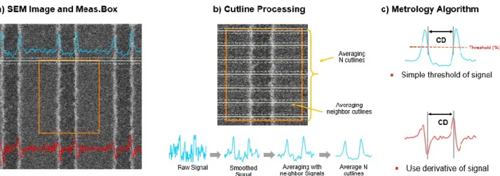
The raw image produced by a scanning electron microscope (SEM) depends on many parameters (e-beam intensity, voltage, scanning direction, the field of view, pixel size, number of frames, distortion…) that have a direct impact on the quality and shape of the signal. A SEM image is basically, a grayscale image highlighting the edges of the measured pattern. Fig. 3 shows an example of the amplitude and derivative of the signal of a cutline for a line and space pattern. The measurement is restricted to a portion of the image, the measurement box (orange rectangle) inside which the signal is analyzed line by line along a cutline. To improve the signal-to-noise ratio, the signal extracted by each cutline (b) is first smoothed (typically low-pass filter) and then averaged with a few neighbor cutlines. Finally, various cleaned cutlines sampled within the metrology window are averaged again to give the final signal that can be processed by the metrology algorithm to derive a pair of edge positions using either the amplitude or the derivative of the signal.
Fig. 3 From SEM image to CD. a) Grayscale SEM image showing a cutline of the signal (amplitude in blue, derivative in
red). b) The signal is cleaned and extracted inside a measurement box (orange rectangle). c) A metrology algorithm is applied to the signal to derive the edge position of the pattern and the CD.
❖ Matching conditions and definition
SEM contours are extracted by processing the signal of the same raw SEM image but with a more sophisticated algorithm to be more robust and versatile because the edge detection is not limited to a portion of the image. Note that a CD measured from contours is just a distance between polygons. Since a critical dimension of a pattern is derived by processing the signal of a SEM image then one can only compare CDs from images of the same substrate acquired with the same settings. In other words, the matching is only valid for a given process and metrology recipe.
More precisely, the matching can be defined for a given SEM image as the difference between a CD measured with the contour and the reference CD (see equation 1). This supposes to work with the same raw SEM image and make sure that the CD derived from the extracted contours is based from the same pixels delimited by the reference measurement box, i.e. with the same size and location (see Fig. 4).
∆𝐶𝐷𝑚𝑎𝑡𝑐ℎ𝑖𝑛𝑔= 𝐶𝐷𝑐𝑜𝑛𝑡𝑜𝑢𝑟− 𝐶𝐷𝑟𝑒𝑓 (1)
Fig. 4 The matching procedure implies using the same SEM image to derive the CD from the conventional SEM-CD
(CD_Ref) and the CD measured from the extracted contour (CD_contour). The size and the position of the measurement box (orange rectangle) must be perfectly matched.
❖ Contour matching flow: calibration and anchoring
The outcome of the matching is ruled not only by the contour extraction process itself, i.e. the effective position of the detected edges, but also by the method to derive the CD from the contours, i.e. the geometry of the measurement box and the cutline sampling. The ASELTA’s contour extraction technology, that we use for this work, has a dedicated flow to ensure enough degrees of freedom for the various matching steps (see Fig. 5). The matching process is divided into two main steps to generate a matching model. First, the contour extraction is calibrated by adjusting a few parameters having an impact on the edge detection position, the contour smoothing, and cleaning. Then, the position of the contour is finely adjusted with a model-based approach to fit a given reference CD, called anchor, using an equivalent measurement box in terms of size, position, and cutline sampling. Several measurements from one or more images may be used for matching, increasing the number of anchors to potentially improve the matching accuracy and its robustness to noise.
Fig. 5 Aselta’s contour matching flow. During the calibration step, the contours are optimized for the edge detection of the
pattern. In a second step, a model-based approach allows a fine adjustment of the contour position to fit a given reference CD (anchor) within the same measurement box (orange).
2.2 Data Preparation
Once a matching calibration model is available, it is used to extract the contours and derive the CDs of a batch of images processed and measured exactly like the anchor. All the matching values coming from each image of the batch are aggregated to evaluate the matching performance and validate the quality of the anchoring model as discussed more in detail in the next section §2.3. For this work, we measured around 200 patterns of various 1D and 2D geometries after lithography and after etch with a dedicated SEM tool. The lithography measurements were also augmented with positive and negative focus conditions. Fig. 6 gives an overview of the patterns, grouped according to their basic geometry. Each group is made of sub-groups representing parametric dimension variations of the group like pitch or linearity modulations. Finally, each single pattern is measured multiple time across wafer at different locations.
Fig. 6 Overview of the data patterns. Each group contains sub-groups generated by geometric parametric variations.
A valid matching necessitates a pair of reliable reference and contour measurements. As illustrated in Fig. 7b, any edge detection error from either the reference or the contour could disqualify the matching value. When looking more into details the variances of the CD_Ref and CD_contour measurement per feature group after lithography (see in Fig. 7a), it appears that in general 2D patterns are showing more CD variation than 1D patterns and the reference measurements suffer more from edge detection problems. This example highlights the importance of identifying and removing outliers before starting a matching analysis. For large image batch, it is not feasible to perform a manual inspection of the pair of measurements. Moreover, the distinction between outliers and valid data points is not obvious. Instead, we propose to remove automatically the outliers based on the property of the matching distribution as shown in Fig. 8. The idea is to keep only the 2%-98% inter-quantiles part of the distribution, with the assumption motivated by the observation that this arbitrary 2% threshold was enough to discriminate between obvious and not obvious measurement errors. This corresponds approximately to removing all measurement pairs with more than +/-6nm of matching value.
Fig. 7: Matching data screening. a) Comparing the variances of the reference and contour measurements for each pattern
Fig. 8: Outliers removal. The distribution of all the matching pairs shows the presence of outliers that can be detected by
considering all the value outside the 2-98% of the inter-quartile range. Inside this range, we observed no obvious measurement errors.
2.3 Matching metrics
Given the CD_Ref and CD_contour measurements of all the SEM images after removal of the outliers and calibration of the anchor model, it is possible to estimate the matching performance by evaluating the correlation between the two components of the dataset. A common method is to use the ordinary least square regression, but it has the drawback to consider that only one variable (y) is subject to error when performing the linear fit (see Fig. 9). A more appropriate method is to recognize that both x and y variables are subject to measurement errors and to take into account their relative variances when performing the regression. Such regression is known as Mandel’s [15, 16] or Deming’s regression [17] and will minimize both x and y errors according to the variance ratio.
Fig. 9: Ordinary Least Square regression considers only error for the y variable, i.e. minimizing the vertical distance
between the points and the fitted line. Mandel Regression takes into account both x and y errors, minimizing a distance at
any angle [0,90°] between the points and the fitted line. Note that if =1 then the distance is orthogonal to the line.
From the Mandel regression, four metrics can be derived to serve as a figure of merits to evaluate and optimize the matching performance between reference measurements and a measurement system under test (TuT):
Mandel Regression Slope (𝜷)̂: it evaluates the difference of sensitivity between TuT and Ref. Unity slope guarantees a good relative accuracy
TMU: From the Mandel regression, one can measure the scatter of the point around the optimal fit line, by computing
the RMS of the residuals, to measure the matching performance of a dataset. However, to evaluate the pure contribution of the SEM-contour measurement uncertainty to the matching error, one has to remove the contribution from the
reference measurement uncertainty. This idea illustrates the concept of TMU (Total Measurement Uncertainty) [18, 19, 16, 20] that was introduced to measure both the precision and the relative accuracy of a tool or system under test (TuT). The relative accuracy refers to the capability of the TuT to follow closely changes in the reference measurement. TMU is a 3-sigma quantity describe by the following equation:
𝑇𝑀𝑈 = 3√𝜎̂ − 𝜎𝑅𝑒𝑔2 ̂ ~ 3𝑅𝑒𝑓2
𝜎𝑇𝑢𝑇
𝛽̂ ̂
(2)
Where 𝜎𝑅𝑒𝑔 2 , 𝜎𝑅𝑒𝑓2 , 𝜎𝑇𝑢𝑇2 are the estimations of the variances of the regression, reference measurement, TuT measurement
and 𝛽̂ the estimation of the regression slope. The measure of the TMU supposes a good estimation of the Ref and TuT measurement variances (or their ratio) which was not available for this work. Instead, we assumed both measurement variances to be equal which is probably a conservative statement especially for 2D patterns which are obviously more prone to measurement errors (see Fig. 7a). To make the estimation of the TMU effective, it is important to restrain it to a particular pattern but with relevant geometric variations potentially affecting the measurement accuracy. For this reason, in this work, the TMU values are computed for each pattern group.
Dataset offset and Std Deviation of the matching: Independently of the regression, these 2 metrics capture any
constant bias in the CD matching distribution.
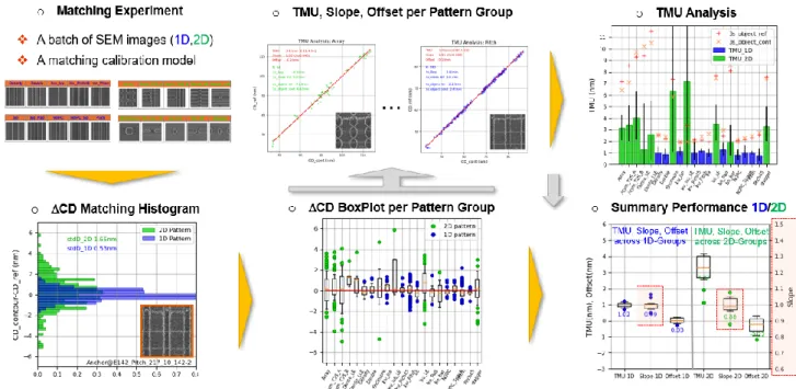
In the experimental section §3, we explore different experiments varying either the batch of SEM images (different processes) or the matching calibration model (model parameters or anchor pattern). Each time, we follow the same methodology to evaluate the matching performances based on the 4 metrics (see above and Fig. 10). First, we plot for a given anchor pattern the matching distribution of all the patterns to identify systematic offset. More details are given by the box-plots representing the matching values per pattern group. Then we run a Mandel regression for each of these groups, to derive the TMU, slope, and offset separating 1D and 2D patterns. Finally, all the metrics can be summarized in a synthetic graph showing in box-plot format, the distribution of the TMU, slope and offset of all pattern groups.
Fig. 10 Matching performance evaluation flow. For each experiment, the TMU, slope, offset and stdD of the matching
dataset is derived per pattern group. Then all the group results are aggregated in a box-plot to get a synthetic view of the matching performance. 𝑂𝑓𝑓𝑠𝑒𝑡 = 𝑦̅̅̅̅̅ − 𝑥𝑟𝑒𝑓 ̅̅̅̅̅̅ (3) 𝑇𝑢𝑇 𝑆𝑡𝑑𝐷 = √∑ ((𝐶𝐷𝑐𝑜𝑛𝑡,𝑖− 𝐶𝐷𝑟𝑒𝑓,𝑖) − 𝑂𝑓𝑓𝑠𝑒𝑡) 2 𝑁 − 1 𝑁 𝑖=1 (4)
3. EXPERIMENTAL RESULTS
In this section, we will investigate the influence of various parameters on the matching performance. In order to get a meaningful comparison, all the matching experiments are run with the same pattern dataset, i.e. measuring always the same patterns at the same location on a wafer.
3.1 Influence of the model calibration parameters
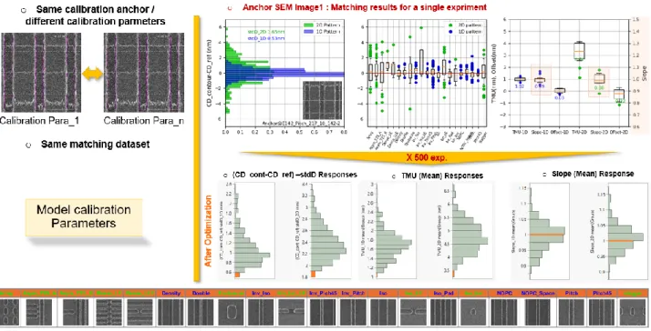
In section §2.1, we described the flow to calibrate a matching model with the help of an anchor image. The model can be tuned with a few parameters that need to be optimized in the first place because they have a strong influence on the matching performance. For that, we run around 500 experiments after lithography with the same anchor to explore the parameter space, allowing each parameter to vary between roughly 0 and 200% of the best guess starting point. The corresponding responses of the matching indicators (TMU, slope, offset, stdD) are compiled in Fig. 11. We can observe a strong spread of the matching performance, highlighting the importance of this first optimization step. Note that this was a blind optimization, meaning no prior knowledge of the reference metrology algorithm.
Fig. 11: Influence of the model calibration parameters.
3.2 Influence of the SEM image pixel size
The purpose of this experiment is to understand how the SEM image pixel sizes influence the matching performance, keeping all other SEM parameters identical. The same isoline pattern was measured after lithography, with rectangular and square pixels (see Fig. 12a). Each image is then used as an anchor to calibrate a “square pixel” and a “rectangular pixel” models (see Fig. 12b). Each model is then cross-validated by measuring the CDs of a limited batch of SEM image with rectangular and square pixels. Fig. 12c shows that there is a very good correlation between the two calibration models, meaning that the pixel size has no significant impact on the matching performance. Note that the pixel size has still a strong impact on the CDs because of the resist shrinkage induced by the SEM e-beam.
3.3 Influence of the pattern geometry: 1D vs 2D
The matching experiments run on section §3.2, after lithography, establish clearly that the 1D pattern groups perform much better than the 2D pattern group. It is interesting to have a closer look at the TMU because it is supposed to measure only the variance of the measurement system and not that of the pattern dimension itself, which is expected to be generally higher for complex shape more difficult to print during lithography (see Fig. 13c). Fig. 13 gives a
comparison of the TMU analysis between a 1D and a 2D pattern groups. The Mandel regression for 1D pattern is around 3 times better than for 2D patterns. This was expected because we observed a much higher rate of measurement errors for 2D patterns, especially for the reference measurement. where the measurement box is much smaller and there are much fewer pixels available to get reliable statistics (see Fig. 13b). For the TMU derivation, we assumed the variances of the reference and contour measurements to be identical (see section §2.3). This is mostly true for 1D patterns where the SNR of the measurement is improved thanks to the large measurement box (see Fig. 13b). However, the TMU is overestimated for 2D pattern because we noticed much more measurement errors of the reference caused by the limited amounts of pixels available to derive the CD. Therefore, in the case of noisy SEM images, 1D images are better candidates to serve as a matching anchor.
Fig. 12: Influence of the SEM image pixel size: (a) The same pattern measured with rectangular or square pixels used to
calibrate 2 models. (b) Each model is validated with a batch of rectangular or square pixel images. (c) The cross-validation of the models shows a good matching.
3.4 Influence of the calibration anchor image
In our dataset, we made sure to have always a few repetitions (8 times) of the very same pattern (see Fig. 6) measured at different locations on the wafer. This gives us the possibility to estimate the influence of the calibration anchor image itself on the matching performance, by calibrating a specific instance of a pattern but with different SEM images with the same matching dataset each time. Fig. 14 shows a significant performance variation between 2 anchors. The Anchor2 is showing clearly a double distribution of the matching values that could be attributed to a symmetrical separation between line and space patterns. By overlaying the available reference edge points (in white in Fig. 14) and the contours (in magenta in Fig. 14) from each anchor image, we can see a very good matching of the edge detection for the first anchor, whereas the second anchor image reveals a few locations with high discrepancy (see orange arrows in Fig. 14 ). Note that the measurement error shifts with the same amplitude the matching distribution of the line and space patterns but with opposite values, which is to be expected because the sum of neighbor line and space -equal to a pitch- remains per definition constant.
Fig. 14: Influence of the calibration anchor image.
The TMU is not affected too much because the main consequence of the localized and limited edge detection errors is to bias the calibration which can be seen as an offset shift in the Mandel regression with limited impact on the correlation itself.
This observation suggests that reciprocally the matching could be improved by biasing on purpose the reference CD of the anchor. Indeed, any measurement error is equivalent to biasing the true CD_Ref of the anchor as illustrated in Fig. 15a. It is then possible to recover the true CD by monitoring the evolution of the matching indicator as a function of the added bias (Fig. 15b, c). The minimum of the curve corresponds to the optimal bias that would compensate at best the edge detection errors. Note: for the sake of the demonstration, we assumed only a measurement error of the reference, but the biasing compensation works actually by combining both contributions of the reference and contour measurement errors.
3.5 Influence of the calibration anchor design
In this section, we want to investigate whether the matching performance can be further improved by selecting an optimal anchor among all the measured patterns. The objective is to determine if specific pattern designs are more suitable for calibration. The study is restrained to 1D patterns, measured after lithography, giving more reliable measurements than 2D patterns. In section §3.4, we have seen that for a given pattern, the matching performance can vary significantly from one SEM image to another. To mitigate this effect, we run around 900 matching calibrations, taking sequentially all the 1D SEM images as an anchor, with a repetition of 8 images per pattern (see Fig. 6). For the sake of clarity, only the matching standard deviations (stdD) are compiled per 1D-pattern group in the box-plot graph of Fig. 16. Confirming the observation of §3.4, it shows that the calibration performance can vary significantly within the same pattern or pattern group. The interesting point is that with enough SEM images, it is always possible to find a good anchor for a given pattern. In addition, this experiment demonstrates that the design of the 1D anchor has no noticeable influence on the matching performance whereas the quality of the measurement for a SEM image does.
Fig. 16 Influence of the anchor pattern design. (a) Plotting the matching standard deviation (stdD) distributions for every
single image of 1D pattern of the dataset taken as an anchor. The box-plots compile the stdD per pattern group. (b) Details of the pattern group ”Double” by plotting the box-plots of the stdD per pattern.
3.6 Influence of the calibration anchor sampling
This brute force analysis of all the possible anchors is not a valid option to optimize the matching because it takes too long to run, but it demonstrates that with enough SEM images, good anchors can be found. Indeed, we propose methods to take advantage of the CD matching distribution to identify the best anchors.
The first method requires 2 iterations of matching calibration with a single anchor and is particularly suited for noisy images with a higher rate of edge detection failure. The first iteration is performed with a random anchor with a given matching distribution signature. Depending on the dataset, it is possible to identify one or two normal distributions corresponding to the line and space patterns. Any pattern with a matching value close to the center of a distribution can be selected as a good anchor candidate for an effective second matching calibration (see Fig. 17b, c).
The second method (see Fig. 17d) is only applicable if the line and space patterns are used and their respective matching distribution centers can be clearly separated because of significant edge detection errors (see §3.4). Following the observations made in section §3.4, we can derive that the distance between the two distribution centers is equal to 2 times the bias that needs to be applied to the reference measurement to compensate exactly for the measurement errors. After biasing the initial anchor CD, the optimized calibration can be run.
Finally, a more rigorous approach consists in considering multiple anchors for the matching calibration. Doing so, the influence of measurement errors of the anchors can be minimized as a result of the statistical effect -assuming the errors to be random. This method is effective only if enough images are sampled to get a good estimation of the matching distribution as illustrated in Fig. 17e, f, g. The best matching performance can be achieved with 900 anchors giving a TMU of around 0.8nm for 1D patterns and 3.2nm for 2D patterns with stdDev of 0.44 nm and 1.52 nm. The regression slope per feature group is also very well centered around unity.
Fig. 17: Influence of the calibration anchor sampling. (a) Taking advantage of a 2 steps calibration to first analyze the
matching distribution to select (b, c) optimal anchors close to the matching distribution centers or (d) assessing a corrective bias for the anchor CD. (e, f, g) Taking advantage of multiple anchor calibration.
3.7 Influence of the lithography focus
In this section, we want to understand whether SEM images measured on patterns printed with different lithography focus conditions are compatible in terms of matching. This question is legitimate as we expect a change of the resist profile as well as a roughness increase for large defocus. For that, we measured the same dataset again on wafers exposed at large positive and negative defocus with identical SEM image acquisition parameters as in the previous experiments. Each time, we compared the matching performance of the dataset measured at a given defocus by using the same anchor pattern measured either at nominal focus or at defocus (see Fig. 18 and Fig. 19). For each run, we selected the best anchor available for the pattern under investigation (see section §3.6). Fig. 18 and Fig. 19 indicate that whatever the defocus, there is no significant difference of the matching performance when using the anchor at nominal focus. This implies that there is no need to redo the matching calibration when changing the lithography focus condition. Note that the overall matching performance is anyhow reduced at defocus because the SEM images are more difficult to measure.
Fig. 18: Influence of lithography negative defocus on the matching performance.
3.8 Influence of the process
The purpose of this last experiment is to compare the matching performance of the very same pattern dataset measured after lithography and after etch. The SEM magnification and the image size are identical in both cases, but the e-beam and frame settings are very different what triggered a preliminary re-calibration of the matching parameters for the post-etch images (see §3.1). Then we evaluated the matching performance with an optimal single anchor selected with a method presented in section §3.6. After etch, we observe much less variability of all the matching indicators, roughly 4 times better matching performance (See Fig. 20) because the patterned edges after etch are much smoother and the image noise much reduced compared to the post lithography condition. The measurement quality is so improved that even 2D patterns measured with a small measurement box can serve as an anchor. Indeed, the example of Fig. 21 shows similar matching performances for 1D and 2D patterns.
Fig. 20: Influence of the process on the matching performance.
4. CONCLUSIONS
In this work, we used a comprehensive dataset of 1D and 2D patterns to investigate the matching between CD-SEM and SEM-contour after lithography and etch. As metrics to evaluate the matching performance, we used the Total Measurement Uncertainty, the slope of the Mandel regression, and the analysis of the matching CD distribution. After running many experiments to assess the parameters influencing the matching performances, we observed that the performances are largely driven by the quality of the SEM measurements (both CD-SEM and SEM-contour) rather than the pattern geometry (pitch, dimension…) of the anchor pattern used to calibrate the matching model. We also noticed that the matching performance is marginally impacted by the lithography defocus but strongly improved after etch. Finally, we propose a few methods to find an optimal matching. They are based either on the analysis of the matching CD distribution of a preliminary calibration or involve multiple anchors for the calibration. Lastly, we have established a method to achieve good matching performance that should facilitate the introduction of SEM contour in a manufacturing environment.
5. REFERENCES
[1] F. Weisbuch and K. Jantzen, "Enabling scanning electron microscope contour-based optical proximity correction models," in J.
of Micro/Nanolithography, MEMS, and MOEMS, 14(2), 021105 (2015). https://doi.org/10.1117/1.JMM.14.2.021105, 2015.
[2] Vasek.J and etal, "SEM-contour-based OPC model calibration through the process window," in Proceedings Volume 6518,
Metrology, Inspection, and Process Control for Microlithography XXI; 65180D, 2007.
[3] F. Weisbuch and A. Naranaya, "Assessing SEM contour based OPC models quality using rigorous simulation," 2014.
[4] Hibino.D and etal, "High-accuracy OPC-modeling by using advanced CD-SEM based contours in the next-generation lithography," in Proceedings Volume 7638, Metrology, Inspection, and Process Control for Microlithography XXIV;, 2010. [5] Wei.C and etal, "Realizing more accurate OPC models by utilizing SEM contours," in Metrology, Inspection, and Process
Control for Microlithography XXXIV;DOI: 10.1117/12.2554527, 2020.
[6] Kuechler.B and etal, "Contour-based model calibration to a minimum number of," in Proc. SPIE 11613, Optical
Microlithography XXXIV, 116130G (22 February 2021); doi: 10.1117/12.2584714, 2021.
[7] Kim.Y-S and etal, "OPC model accuracy study using high volume contour based gauges and deep learning on memory device," in Proceedings Volume 10959, Metrology, Inspection, and Process Control for Microlithography XXXIII; 1095913, 2019. [8] Wei.C and etal, "Realizing more accurate OPC models by utilizing SEM contours," in Proceedings Volume 11325, Metrology,
Inspection, and Process Control for Microlithography XXXIV; 1132524, 2020.
[9] Lakcher.A and etal, "SEM contour based metrology for microlens process studies in CMOS image sensor technologies," in
Proceedings Volume 10587, Optical Microlithography XXXI; 105870T;, 2018.
[10] Weisbuch.F and etal, "Calibrating etch model with SEM contours," in Proc. of SPIE Vol. 9426 94261T-2;· doi:
10.1117/12.2180271, 2015.
[11] Weisbuch.F and etal, "Characterizing interlayer edge placement with SEM contours," in J. of Micro/Nanolithography, MEMS,
and MOEMS, 18(2), 021203, 2019.
[12] Lakcher.A and etal, "Advanced metrology by offline SEM data processing," in Proceedings Volume 10446, 33rd European Mask
and Lithography Conference; 104460L, 2017.
[13] Le-Gratiet.B and etal, "Contour based metrology: “make measurable what is not so"," in Proceedings Volume 11325, Metrology,
Inspection, and Process Control for Microlithography XXXIV;, 2020.
[14] Fischer.D and etal, "Challenges of implementing contour modeling in 32nm technology," in Proceedings Volume 6922,
Metrology, Inspection, and Process Control for Microlithography XXII; 69220A (2008), 2008.
[15] J. Mandel, "Evaluation and control of measurements," in Quality and Reliability Series, 1991. [16] B. Bank and C. Archie, "Characteristics of accuracy for CD," in SPIE Vol. 3677 • 0277-786X/9, 1999. [17] "Deming regression," Wikipedia, 2021. [Online]. Available: https://en.wikipedia.org/wiki/Deming_regression.
[18] Hartig.C and etal, "Practical aspects of TMU based analysis for," in 40th International Convention on Information and
Communication Technology, Electronics and Microelectronics (MIPRO), 2017.
[19] Rana.N and etal, "The measurement uncertainty," in Proc. of SPIE Vol. 7272 727203-1, 2009.
[20] R. Weed and R. Barros, "Demonstration of Regression Analysis with Error in the Independent Variable," in Transportation