HAL Id: inria-00345954
https://hal.inria.fr/inria-00345954
Submitted on 11 Dec 2008
HAL is a multi-disciplinary open access
archive for the deposit and dissemination of
sci-entific research documents, whether they are
pub-lished or not. The documents may come from
teaching and research institutions in France or
L’archive ouverte pluridisciplinaire HAL, est
destinée au dépôt et à la diffusion de documents
scientifiques de niveau recherche, publiés ou non,
émanant des établissements d’enseignement et de
recherche français ou étrangers, des laboratoires
Multi-agent Systems as Discrete Dynamical Systems:
Influences and Reactions as a Modelling Principle
Vincent Chevrier, Nazim Fatès
To cite this version:
Vincent Chevrier, Nazim Fatès. Multi-agent Systems as Discrete Dynamical Systems: Influences and
Reactions as a Modelling Principle. [Research Report] 2008. �inria-00345954�
Multi-agent Systems as Discrete Dynamical
Systems: Influences and Reactions as a Modelling
Principle
Vincent Chevrier and Nazim Fat`
es
∗Nancy Universit´
e – INRIA Nancy Grand-Est – LORIA
December 10, 2008
Abstract
Finding adequate descriptions of multi-agent systems is a central issue for modelling collective dynamics. We propose a mathematical description of multi-agent systems as discrete dynamical systems. The ground of our proposition is the influence-reaction method of Ferber and M¨uller. The key idea is that agents should never act directly on other components of the system (agents or environment) but release influences which are then combined to update the state of the system. We propose a method which decomposes the definitions of multi-agent system into six parts: (1) the basic sets, (2) the perception of the agents, (3) the influences, (4) the updating of the agents’ internal state, (5) the updating of the environment, (6) the updating of the position and observable states of the agents. We illustrate our method on the multi-Turmite model, also known as the multiple Langton’s ants model. We exhibit two formulations of this model, which we study with three different simulation schemes. We show that for the same formulation, and the same initial conditions, the use of different simulation schemes may lead to qualitatively different evolutions of the system. As a positive spin-off of this study, we exhibit new phenomena of the multi-Turmite model such as deadlocks or gliders.
Keywords: multi-agent systems ; discrete dynamical systems ; collec-tive dynamics modelling ; Langton ants.
1
Introduction
The thesis of this paper is that multi-agent systems should be described and analysed by clearly separating, on the one hand, the description of
∗corresponding author: INRIA Nancy Grand-Est - Campus scientifique - CS 20101 - 54603
the agents, and, on the other hand, the simulation scheme. By “simula-tion scheme”, we mean all the opera“simula-tions that regard the update of the components of a system, by opposition to the local laws that define the behaviour of each component. We consider such a separation as a means of answering two questions:
• How to describe a multi-agent system with a mathematical formal-ism that removes ambiguities of formulation and that allows readers to reproduce an experiment with precision?
• To which extent does the global behaviour of a multi-agent system depend on the laws governing the agents and to which extent does it depend on the simulation scheme used to update the system? To give a metaphor, let us consider an orchestra where musicians have to perform a concert. Clearly, giving each musician its partition is not sufficient. How to write this partition so that they can play together? Can they play without listening to the other musicians? Should they play independently for some time and get together at some specific moments? When can they play freely and when do they need to follow a chief con-ductor? etc. These questions can of course be raised for many types of dynamical systems. The case of multi-agents is especially interesting since it involves a great number of entities, which are of two types: the agents and the cells of the environment. A dedicated formalism is needed to ensure that the agents and the environment “play the right partition”.
There exists a wide variety of formalisms to describe multi-agent sys-tems, each devoted to a given architecture of agent. Agents are said situated when they are located in a shared environment (they have a po-sition), when they perceive it and can act upon it. It is common to divide the agents types into the reactive agents with a small memory and limited reasoning, and the cognitive agents, which possess an internal (partial) image of their environment and are able of making reasoning and deduc-tions [19, 21]. In this article we will consider only situated and reactive multi-agent systems: agents do not communicate directly by messages and their behaviour is equivalent to reflex rules.
Our proposition is to take the influence-reaction method of Ferber and M¨uller [12] as a basis for describing situated and reactive multi-agents. The key idea is that agents do not act directly on their environment but rather produce influences, which modify the environment and the agents. This method is particularly useful when one needs to employ a synchronous updating of the system. Our description aims at removing the ambiguities that could appear if the description of the system were given in pseudo-code or in a specific programming language. This influence-reaction method allows its followers to easily deal with the “conflicts” or “combinations” resulting from simultaneous actions of agents. Loosely speaking, our formalism might be seen as taking a step further the idea of Ferber and M¨uller of considering multi-agent systems as discrete dynam-ical systems.
In our proposition, we decompose the description of a system by considering a collection of state vectors (the environment components, the agents’ positions, the agents’ states) that evolve according to well-defined functions (as opposed to computer procedures). More precisely,
the method is to decompose the definition of multi-agent system into six parts: (D) the definition of the basic sets, (A1) the agent’s perception, (A2) the agent’s production of influences, (A3) the agent’s internal updat-ing, (SE) the updating of the environment and, (SA) the updating of the positions and observable states of the agents. The steps (A1), (A2), (A3) define the laws related to the reduction of information from a global point of view to a local one. The steps (SE) and (SA) define the laws related to the inverse operation, from local to global, which consists in collecting influences and combining them to solve potential conflicts created when agents act simultaneously on the same components.
2
Related works
An import topic in the multi-agent field regards the mathematical de-scription of these systems [19, 21]. Several authors have worked to estab-lish a separation between the expression of the behaviour of the agents and the simulation scheme. Ferber and M¨uller proposed the influence-reaction model as a first attempt to separate tentative actions from the environment reaction [12]. Following this direction, F. Michel proposed a computational model that follows the influence-reaction principles [16]. This work was then precised by a formal framework which represents the environment as “a dynamical system that encapsulates and regulates its own dynamism” [14]. These propositions aim at removing the ambigui-ties of description that exist when a multi-agent system is described only with a computer language. However, the question to know how much the simulation scheme contributes to the global behaviour of the system is rarely considered.
On the other hand, there are several works which concern multi-agent systems [1, 4, 20, 18] or cellular automata [6, 11] where the authors have focused on evaluating the effect of the updating scheme on the global behaviour of the system. They considered several variations in the updat-ing scheme and demonstrated that it has an important influence on the global outcome of a simulation. In the case of cellular automata, it was even shown that minor changes in updating scheme can produce substan-tial ones at global level [10, 9]. In most of these works, the main concern of the authors is to evaluate changes of behaviours but not necessarily to propose a formal description that allows to test for a wide varieties of simulation strategies.
In short, it appears that authors so far have focused their efforts either on the formalisation side (how to describe mathematically multi-agent systems?) or on the experimental side (how does the updating scheme affects the outcome of a simulation?). In this article, we propose to com-bine these two questions to perform an analysis of a simple multi-agent system, namely, the multi-Turmite system.
3
Turmites as Case Study
In this paper, we illustrate our method by focusing on a simple model. The agents evolve on a grid; their actions are limited to: (1) moving forward, (2) turning left or right and, (3) inverting the state of the cell on which they are located (an operation that we call flipping the cell). The most popular expression of the system was proposed by C. Langton in his pioneering paper on “artificial life” [15]. In Langton’s view, we can gain insights on how living organisms obtain there distinguishing properties -as opposed to inert matter - by modelling an “artificial biochemistry” that would rely on interactions between “artificial molecules”. These artificial molecules are modelled by virtual automata, whose behaviour is specified by simple rules that only rely on local interactions. Among many examples given by the author, a proposition concerns the study of artificial “insect colonies” where the insect, called vant (for virtual ant), obeys the simple rules [15]:
◮The vant moves on a square lattice where each cell can be blue or yellow; cells are initially all blue.
◮If it encounters a blue cell, it turns right and leaves the cell coloured yellow.
◮If it encounters a yellow cell, it turns left and leaves the cell coloured blue.
As pointed out by A. Gajardo, this model was also discovered, indepen-dently by other authors, among whom L. Bunimovich and S. Troubetzkoy [3], and A. Dewdney [7] , who described the agents as Turmites. We adopt this name in the following of the article as it underscores that each Tur-mite, when considered isolated from the other Turmites, is an example of a Turing machine that operates on a two-dimensional tape.
Authors observed that these simple rules produced a complex be-haviour even when the system is composed of a single ant. Before going further, readers who are not familiar with this system should perform a few simulation steps “by hand”. This small exercise is rather puzzling since predictions of behaviour are difficult to extend beyond a few time steps. One reason for this difficulty stands in the absence of clear repetitive pat-terns: a Turmite passes through the same positions again and again but leaves a different trail behind it at each of its return. Long time simula-tions show that the behaviour of the Turmite does not stay “chaotic” for ever: after ∼ 10 000 time steps, it enters into a cyclic behaviour where it repeats the same relative moves forever. These repetitions result in a reg-ular displacement in one of the four diagonal axes, leaving a “self-limited pathway” behind it.
Figure 1-left illustrates the evolution of a single Turmite on a grid that is initially empty. In order to show the sensitivity to the initial condition of the system, we flipped the cell (0, 1). Figure 1-right shows the evolution of the system for this new initial condition. We observe that the Turmite also reaches the “pathway regime”, but at an earlier time (t ∼ 3 000). This experiment underlines how small changes may affect the evolution of the system. This property of sensitivity to the initial condition will be useful for demonstrating the benefits of separating the description of
t= 11500 t= 3000
Figure 1: Evolution of a single Turmite from position (0, 0, North): (left) Initially, all cells are in state 0; (right) Same initial condition, except that the cell (0, 1) is set in state 1 (e(0,1)= 1). 0-cells and 1-cells are displayed in white
and blue (or dark), respectively. Turmites appear in red (or grey) but is by no means important. Simulations were produced by the FiatLux simulator [8].
a model and its execution scheme.
The study of the behaviour on a single ant gave rise to numerous studies and readers may refer to the work of Gajardo et. al. for an overview (see e.g. [13]). Now we examine a question that has been much less examined: what happens when several ants are put together? To our knowledge the only references that considered multiple Turmites are the work of Chopard and Droz [5] and the paper by Beuret and Tomassini [2]. Remark that before we study this model, we need to specify how Turmites interact. According to Langton’s own words [15]: “ There are so many ways that these virtual ants can encounter one another that the transition rules have not yet been worked out for all possible encounters.” This lead him to propose to adopt the simple strategy that consists of leaving the ants “pass through each other” and react to the cells’ state without taking account of the other Turmites.
We may note that although the solution is perfectly acceptable, the problem of dealing with multiple ants is only half-solved. Indeed, how should simulation programs operate in the case where several Turmites share the same cell and simultaneously change the state of their cell? As nothing is specified, we are allowed either to choose arbitrarily, or, what is wiser, to believe that the implicit assumption of the author is that the updating of the agents is sequential: Turmites (and their cells) are always updated one after the other in a fixed order. However, it a is well-known problem that this method of taking a sequential updating of agents is by no means a panacea:
• Ambiguities in the model exist if the order of updating is not well-specified. As a consequence, the reproduction of experiments with different simulation environments is made difficult, if not impossible.
• Even in the case where the updating scheme is well-specified, it may introduce an artificial causality and create unwanted effect such as biases in the simulation or an artificial symmetry breaking (see later for examples).
Our purpose is to illustrate, on the case of Turmites, a method to specify independently how the agents behave and how to execute the simulation with many agents. In particular, we provide a description of a synchronous updating of multiple Turmites and their environment. But before we go further, let us reformulate the behaviour of Turmites with a new perspective, intended to facilitate its transcription with influences and reactions:
◮Each cell in the environment can be in state 0 or 1. ◮If a Turmite finds a 0-cell it attempts to flip the cell, to turn right and to move forward.
◮If a Turmite finds a 1-cell it attempts to flip the cell, to turn left and to move forward.
As readers might have noticed, this rewriting of the rules not only takes the agent’s perspective but also describes the behaviour of the agent in terms of attempts, or influences, rather than in terms of effective actions. The next section describes how to capture this idea in a mathematical way with the discrete dynamical systems point of view.
4
Describing Multi-agents as Discrete
Dy-namical Systems
Our convention is to use ‘calligraphic’ letters for the basic sets E, P, O, I. We use vectors for denoting collections of such sets (e.g., ~E ). We use lower case for instances of sets, (e.g., o ∈ O ); vectors denote ordered collections of such elements (e.g., ~o ∈ ~O ).
4.1
Foundations
We define a reactive discrete multi-agent system as an association of a col-lection of static cells, the environment, and a colcol-lection of mobile entities, the agents. Space is modelled by the regular square grid Z2 in which each cell c = (cx, cy) ∈ Z2 is associated to a state. The set of possible states
for each cell is E. An environment ~e is an assignation of a state to each cell, the set of all possible environments is ~E = EZ2
.
The agents are entities that evolve by acting on the environment and by interacting together. Let A be the number of agents; for the sake of simplicity, we will consider that it is fixed over time.
Agents are situated and we associate to each agent a a position pa ∈
P = Z2 on the grid. The collection of the positions of the A agents is
denoted by ~p ∈ ~P = PA. Note that we adopt two different notations for
positions and cells even though the two sets are here equal. This semantic distinction should ease the exposition of the formalism, allowing readers to see directly when cells are considered as positions and when they are
considered as components of the environment. This distinction may also have a counterpart in the coding of our formalism in a computer language but this issue is out of scope of the present article. Also note that in a more general framework, one could imagine that the positions of the agents are continuous while their environment is discrete.
We divide the state of an agent into two categories, the internal and observable states:
• The internal state is the information that an agent can modify di-rectly without taking into account the other agents or the environ-ment. Internal states are neither “visible” by the environment nor by the other agents. Examples of typical internal states would be an agent’s time counter or a memory of the last decision taken. • The observable state is the information that an agent have to share
with other components (environment and other agents). By defini-tion an agent cannot modify it by itself; an agent can only produce influences that will modify observable states according to a reaction of the system. Typical observable states are signals sent to other agents. For example, if we need to model a bad reception of a signal from an emitter agents to a receiver agent, we should not allow the emitter agent to modify directly the state of the receiver agent. Note that in many cases the decision to put an information as an internal or observable state is somehow ad hoc. This choice depends mainly on what we need to observe in this model. In the next sections, we will illus-trate this freedom of modelling by presenting and analysing two models of the same behaviour, but with different modelling choices.
4.2
Discrete Updating the System
The set of observable states is denoted by O, the set of internal states by I. The sets of the observable and internal states of the A agents are ~O = OA
and ~I = IA, respectively. We denote by ~σ = (~e, ~p, ~o,~i) ∈ ~E × ~P × ~O × ~I
the given state of a MAS where:
• ~e ∈ ~E represents the state of the environment,
• ~p ∈ ~P represents the sequence of positions of the A agents,
• ~o = ` o1, . . . , oA´ ∈ ~O represents the observable states of the A
agents,
• ~i =` i1, . . . , iA´ ∈ ~I represents the internal states of the A agents.
We suppose that these vectors are updated with a discrete time updating function. A simulation step is obtained with ~σ(t+1) = SystemUpdateˆ ~σ(t) ˜; the SystemUpdate function is calculated by using four steps:
(1) The perceptions of agents at time t are calculated with: ~π(t) = Perceiveˆ ~e(t), ~p(t), ~o(t) ˜
(2) The computation of the influences produced by agents is obtained with:
(3) The new internal state of agents is obtained with: ~i(t + 1) = AgentUpdateˆ~i(t), ~π(t) ˜
(4) The new state of the environment, the new positions and the new observable states of the agents are given by:
(~e, ~p, ~o)(t + 1) = Evolveˆ (~e, ~p, ~o, ~γ)(t) ˜
We now examine with more details how to express the four functions Perceive, Decide, AgentUpdate and Evolve.
4.3
Autonomy and Homogeneity of Agents
The multi-agent perspective leads us to express the functions Perceive, Decideand AgentUpdate as the collection of A functions specific to each agent. In other words, the autonomy of the agents is translated formally by describing these three functions as the product of independent local functions, e.g., ~π = (πa)a∈{1,...,A}with:
πa(t) = Perceiveaˆ ~e(t), ~p(t), ~o(t) ˜
This formulation explicitly forbids an agent a to use the perception of another agent a′. Decisions are also made independently according to:
γa(t) = Decideaˆ ia(t), πa(t)˜
As the internal state is updated by the agent without any constraint from the environment or from the other agents, its value is set according to:
ia(t + 1) = AgentUpdateaˆ ia(t), πa(t)˜
Intuitively, we would define as homogeneous a system whose agents are all identical. Note that as the perception depends on the position of the agents, it is not possible to define homogeneity by simply requiring that the functions Perceivea, Decidea, and AgentUpdateado not depend
explicitly on a. A formal definition of a homogeneous system is available in the Annex (see page 30).
4.4
Locality in the Perceptions of Agents
The perception function Perceivea defines what part of the system has
a direct effect on an agent a. In general, the agents’ perception is limited to its neighbouring environment and to the observable states of the neigh-bouring agents. The neighneigh-bouring components are defined with functions that depend only on the information located around the agents’ position pa. Formally speaking, Perceiveaassociates to an environment, a set of
positions and observable states of agents a value in a set denoted Perc: Perceivea: ~E × ~P × ~O → Perc
The set Perc represents all the possible information that an agent might access in his “neighbourhood”. In order to keep our formal framework open, we purposely do not further specify how this neighbourhood should be defined; however, it is easy to see that it can be formally expressed with the graph distance between the positions in the grid Z2.
4.5
From Perception to the Behaviour of an Agent
How are the perceptions used to define the “behaviour” of an agent? Following the influence-reaction method, we model the behaviour as a production of influences and the updating of the internal state.
The production of influences is made following: Decidea: I × Perc → Infl
(i, π) → γ
In other words, each agent produces an influence γ ∈ Infl as a function of its internal state i and its perception π. The influences produced by different agents will be combined by the global system and act on its evolution. Note that we can divide influences into three categories: (1) the “requests” of the agents for modifying their own observable state (e.g., “I want to turn and move forward”), (2) the requests which concern other agents (e.g., “push neighbouring agent”), and (3) the “requests” on their environment (e.g., “I want to flip the state of my cell”). We require that the set of influences Infl contains at least the null influence, denoted by ⊙, whose effect is to leave the agent and the environment in the same state.
The updating of the internal states is made following: AgentUpdatea: I × Perc → I
(i, π) → i′
Defining AgentUpdatea should be rather straightforward as internal
states do not directly influence the behaviour of the system. Their ef-fect is indirect, they are a type of memory, that operates on how the agent’s decisions are made.
4.6
Conflicts Resolution: From Influences to
Ef-fects on the System
With a synchronous updating, the global transition of the system from time t to t + 1 is simply obtained with the function:
Evolve: E × ~~ P × ~O × InflA → E × ~~ P × ~O
(~e, ~p, ~o, ~γ) → (~e′, ~p′, ~o′)
There are of course various ways of expressing this function, the most in-tuitive way being to decompose the calculus of each component separately. In the next section, we will take another approach and define the multi-Turmite system with intermediary functions and variables. This simplifies the reading of Evolve and to prevent useless repetitions of computations. In the case where we do not update simultaneously all the components of the systems at each time step, we need to define an asynchronous updating of the system. For example, a possibility to define a sequential updating is to take into account only the influence of the agent to update and to artificially set the other influences to the ⊙ influence. We give the formal description of the sequential updating scheme in the Annex (see page 30).
4.7
Synthesis: A Method for Describing Models
We proposed a method to express multi-agent systems as with the formal-ism of discrete dynamical systems. The elements required for expressing a model are summed up in Table 1. Note that none of the functions used to specify the system’s behaviour explicitly depend on time. This restric-tion yields us to include all the time dependencies in the internal state of agents. For example, if agents depend on batteries that have a limited lifetime, then this lifetime has to be explicitly considered as part of the agents’ internal state. The next two sections propose an illustration of this method ; each section is devoted to study a different choice on how to model the multi-Turmite model.
5
First Multi-Turmite model
We now study how to describe the multi-Turmite model with our method. In this first interpretation of this model, we suppose that each Turmite has a ”sense of orientation”: it is able of choosing its own direction without any constraint from the environment, this direction is thus modelled as an internal state.
5.1
Modelling Part
Step (D) Let us first define the basic sets of the model. The environ-ment is made of cells that are passive and binary: E = {0, 1}. We denote the four cardinal directions by D = {North, East, South, West}. The set of internal states of an agent is I = D; it represents the orientation of the agent. As we need no other information to model the problem, the set of observable states is here empty: O = ∅.
Step (A1) The set of perceptions is Perc = E. An agent perceives only a state of according to:
Perceivea: E × ~~ P × ~O → Perc (~e, ~p, ~o) → π
where π = epa is the state of the cell on which agent a is located.
Step (A2) The set of influences Infl = InflF × InflD is composed of two parts. The first set InflF = {Flip, NoFlip} represents the influ-ences on the cells: “flip” or “no flip” influence. The second set InflD = {ToN, ToE, ToS, ToW, Stay} represents the attempts of moves of the agents (“go to direction X” or “stay”). The null influence is defined as ⊙ = (NoFlip, Stay). The decision function writes:
Decidea: I × Perc → Infl
(i, 0) → ` Flip, To(Right(i)) ´ (i, 1) → ` Flip, To(Left(i)) ´
where each element i ∈ D is associated to the Left(i) and Right(i) operations expressing left or right turn respectively to i, for example
Table 1: Notations and method to describe a model
Sets:
Z2 . . . Set of cells (grid) E . . . Set of states for each cell ~
E= EZ2
. . . Environment P = Z2 . . . Position of agents I . . . Internal states of agents O . . . Observable states of agents Perc . . . Set of perceptions Infl . . . Set of influences
Functions:
Perceivea: ~E × ~P × ~O → Perc . . . Perception function of an agent Decidea : I × Perc → Infl . . . Decision function of an agent AgentUpdatea: I × Perc → I . . . Internal state updating of an agent Evolve: ~E × ~P × ~O × InflA→ ~E × ~P × ~O . . . Updating of the system
Steps of the method:
(D) Define basic sets of the model: the environment E, the agent’s internal states I and observable states O.
(A1) Define the agent’s set of perception Perc and its perception function Perceivea.
(A2) Define the agents’ set of influences Infl and its decision function Decidea.
(A3) Define the agents’ internal updating function AgentUpdatea.
(S) Define the system’s global transition function Evolve. The definition of this function may be split into two parts:
(SE) Define the new state of the environment.
Left(East) = North. The function To(d) associates to each direction d its corresponding influence, for example To(North) = ToN.
Step (A3) An agent updates its internal state freely according to: AgentUpdatea: (I × Perc) → I
(i, 0) → Right(i) (i, 1) → Left(i)
5.2
Simulation Part
Recall that we define the simulation part with the function: Evolve: E × ~~ P × ~O × InflA → E × ~~ P × ~O
(~e, ~p, ~o, ~γ) → (~e′, ~p′, ~o′)
We now express simulation schemes by giving different definitions of the three components ~e′, ~p′, ~o′ provided the four components ~e, ~p, ~o and ~γ.
These definitions necessitate to transform influences into effective modifi-cations of the system. In the case of the multi-Turmite model, we separate the definition of the simulation scheme into two parts: (a) the updating scheme, which will be synchronous or sequential (b) the influence manage-ment policy, which defines how to deal with conflicts created by influences which operate on the same elements. We only consider the conflicts cre-ated by simultaneous attempts to move on a single cell.
Definition of step (SE) The first step (SE) consists in calculating, for each cell c, the new state of this cell e′
c according to the influences
produced by the agents. The new state depends on how many flips are applied on this cell. In a free interpretation of the multi-Turmite model, we arbitrarily choose to apply the Fusion influence management policy, in which flips applied simultaneously on a cell combine into a single flip. Of course, another simple choice would be to apply an Annihilation policy, where the simultaneous flips annihilate by pairs (see [5]). Formally, given a couple of positions and their associated influences (~p, ~γ), the “flip counting function” CountFlip[c] writes:
CountFlip[c] : P × Infl~ A
→ N
(~p, ~γ) → card{a ∈ A , (pa, γa.1) = (c, Flip)}
where γa.i denotes the i-th element of γa. The evolution of an environment
cell is then given by:
(SE) e′c=
(
1 − ec if CountFlip[c](~p, ~γ) > 0
ec otherwise
Note that the definition of o′
a, is here unnecessary as the observable
state is empty. To perform step (SA), we now present two different influ-ence management policies for the calculus of p′
Step (SA): the Allow policy The Allow influence management pol-icy consists in handling multiple influences without applying any exclusion principle. The new position of the agents ~p′is thus defined independently
for each agent a with:
p′a= pa+ Move(γa.2)
where the Move function associates an influence of relative move to an offset on the lattice:
Move: InflD → Z2 Stay → (0,0) ToN → (0,1) etc.
Figure 2 presents a comparative evolution of three systems with four Turmites arranged in square: the agents are placed in the following posi-tions: (0, 0, North), (4, 0, North), (4, 4, South), and (0, 4, South), with their respective order 1,2,3,4. The three systems are defined with the Allowpolicy, but with three different updating schemes: (left) synchronous updating, (middle) sequential updating with order 1-2-3-4, (right) sequen-tial updating with order 1-3-2-4. We observe that the synchronous up-dating preserves the central symmetry of the initial pattern while the sequential updating breaks this symmetry in two different ways, depend-ing on which the updatdepend-ing order is chosen. The asymptotic evolution of the three systems is different: the synchronous systems produces four pathways in four different directions, while the sequential systems evolve with no symmetry. This experiment illustrates the artificial biases that can arise when we update the agents one after the other in an arbitrary order (see also ref. [2] for similar observations). Interestingly, if the initial distance between agents is set to 5 instead of 4, all the three systems have the same execution ; in particular, no symmetry breaking is observed (not shown here).
In order to stay with a simple model, we now limit our scope to syn-chronous updating, leaving the study of other updating policies for further work. We denote by < Model M, Pol > a system defined with model M with synchronous updating and influence management policy P ol. Note that the Allow influence management policy was the only policy consid-ered so far by authors who studied a multi-Turmite model [15, 5, 2]. Let us now examine another policy.
Step (SA): The Exclude policy The strong exclusion policy consists in allowing an agent to move to a target cell if and only if this target cell contains no agent and if there is only one agent attempting to move to this cell; otherwise, the move is forbidden.
The problem is now to compute ~p′ by taking into account all the
attempts to move to a same target cell. Given a couple of associated positions and influences (~p, ~γ), we denote the target cell of an agent a by ˜
pa= pa+ Move(γa.2). We then introduce a “presence counting function”
CountPresence[c] such that:
CountPresence[c] : P~ → N ~
t= 0 t= 0 t= 0
t= 50 t= 50 t= 50
t= 89 t= 89 t= 89
t= 90 t= 90 t= 90
t= 13000 t= 2000 t= 3000
Figure 2: Comparison of three systems with initial condition: (0, 0, North), (4, 0, North), (4, 4, South), and (0, 4, South). (Left) < Model 1, Allow > with synchronous updating (Middle) < Model 1, Allow > with sequential updating 1-2-3-4. (Right) < Model 1, Allow > with sequential updating 1-3-2-4.
and a “move counting function” CountMove[c] that counts the simulta-neous influences which have cell c as a target:
CountMove[c] : P × Infl~ A → N
(~p, ~γ) → card{a ∈ A , ˜pa= c}
We can now define the Exclude policy by introducing the predicate IsFree[c](~p, ~γ) which tells whether Turmites might access to cell c given a couple (~p, ~γ):
IsFree[c](~p, ~γ) ⇐⇒
CountPresence[c](~p) = 0 and CountMove[c](~p, ~γ) = 1 The new position of an agent a is then given by:
p′a=
( ˜
pa if IsFree[˜pa](~p, ~γ)
pa otherwise
Clearly, we may define many other influence management policies, such as choosing one agent randomly to move and blocking all the others. For the sake of conciseness, we limit our study to the Allow and Exclude policies.
5.3
A First Comparison of the Two Policies
As a preliminary remark, we wish to draw the attention of the reader that in case of a single ant, an initial condition leads to the same evolution of the system whatever the model, the policy and the updating are.
Figure 3 shows the evolution of the system with two Turmites and with the Allow (left) and Exclude policy (middle). The system is composed of two agents initially located at positions (0, 0, South) and (2, 0, North). Initially, all cells are in state 0.
For the four first steps of the simulation, as there is no interaction between the agents, the two systems evolve identically. The divergence appears at time t = 5 when two agents attempt to go on the same cell. From that time, the evolution of the two systems diverges. Eventually, we find that their asymptotic evolution is qualitatively similar (two paths are created), but it is quantitatively different: the two paths appear at different time steps and have different directions.
This small experiment illustrates how the use of two simulation schemes may lead to different evolutions even though the agents have the same def-inition. We now examine a second model, in which the expression of the Turmites’ orientation is modified.
6
Second Multi-Turmite model
In this second model, Turmites are no longer supposed to have a sense of orientation. All they can do is to make attempts to move forward and attempts to turn left or right. These attempts can be either realised or forbidden by the laws of the environment. As opposed to the first model where Turmites could choose freely their orientation, this new model is more adapted to modelling real agents such as robots.
t= 0 t= 0 t= 0
t= 4 t= 4 t= 4
t= 5 t= 5 t= 5
t= 6 t= 6 t= 6
t= 2500 t= 6200 t= 7500
Figure 3: Comparison of three systems with initial condition: (0, 0, South) and (2, 0, North). (Left) < Model 1, Allow > (Middle) < Model 1, Exclude >. (Right)< Model 2, Exclude >.
6.1
Modelling Part
Step (D) The environment is not changed: E = {0, 1}. The agents are now defined with the set of internal states as I = ∅, and the set of observable states as O = D.
Step (A1) The perception of an agent is identical to those of Model 1; we have Perc = E and
Perceivea: E × ~~ P × ~O → Perc (~e, ~p, ~o) → π
where π = epa is the state of the cell on which agent a is located.
Step (A2) The set of influences is now Infl = InflF × InflT × InflM. The set InflF = {Flip, NoFlip} is identical to the previous model’s. The set InflT = {Tleft, Tright, NoTurn} represents the “turn left”, “turn right”, “no turn” influence. The set InflM = {Fwd, Stay} represents the “go forward” or “stay” influence. The null influence is defined as: ⊙ = (NoFlip, Stay, NoTurn). The Decidea function is now:
Decidea: Perc → Infl
0 → (Flip, Tright, Fwd) 1 → (Flip, Tleft, Fwd)
Step (A3) Since the set of internal states is empty, the AgentUpdatea
function is empty.
We emphasise that although the definitions of steps (A2) and (A3) are different than for Model 1, the formalisation expresses the same individual behaviour of agents. Let us now examine what are the differences in terms of influence management policies.
6.2
Simulation Part
Recall that the Evolve function defines the simulation scheme: Evolve: E × ~~ P × ~O × InflA
→ E × ~~ P × ~O (~e, ~p, ~o, ~γ) → (~e′, ~p′, ~o′)
Again, we split the definition of the simulation scheme into two parts.
Step (SE) The calculus of ~e′for the evolution of an environment cell is
identical to the first model (see Sec. 5.2).
Step (SA) To compute the new position p′
a and the new observable
state o′a, of an agent a we first introduce the target orientation ˜oadefined
by:
˜
oa= Turn(oa, γa.2)
where Turn associates a direction and a rotation to a direction: Turn: D × InflT → D
(W,Tleft) → S (N,Tright) → E etc.
The target cell of an agent a is computed according to: ˜
pa= pa+ Offset(˜oa)
where the Offset associates a direction to an offset on the lattice: Offset: D → Z2
N → (0,1) E → (1,0) etc.
Note that Offset operates on D whereas Move met in Sec. 5.2 operates on InflD. We now express the different policies that define the step (SA).
Step (SA): the Allow policy The updated position p′aand observable
states o′
ais written simply as:
(p′a, o′a) = (˜pa, ˜oa)
Fact 1 (First Equivalence) The systems < Model 1, Allow > and < Model 2, Allow> are equivalent.
This equivalence results from the systematic validation of the influences without applying any constraint from the environment.
Step (SA): the Exclude policy As for Model 1, we define this policy by applying a strong exclusion principle: the state of an agent is not modified as soon as a conflict appears. We have:
(p′a, o ′ a) = ( (˜pa, ˜oa) if IsFree[˜pa](~p, ~γ) (pa, oa) otherwise
The predicate IsFree[c] is defined as in the previous section. Note that as the set of influences has changed, the set of definition of IsFree[c] and CountMove[c] changes accordingly. However, the notations are identical. Fact 2 The systems < Model 1, Exclude > and < Model 2, Exclude > are not equivalent.
The difference between both systems comes from the status of the ori-entation. In case of conflict, in Model 1, the orientation of a Turmite is modified, while it remains unchanged in Model 2. The divergence of behaviour between the two systems is illustrated on Fig. 3-middle and Fig. 3-right.
Step (SA): Turn & See policy This case is more interesting since we can now introduce the possibility for an agent to turn but not to go forward when a conflict appears. In this case, we update the agent’s position and observable state with:
(p′a, o′a) =
(
(˜pa, ˜oa) if IsFree[˜pa](~p, ~γ)
(pa, ˜oa) otherwise
Fact 3 The systems < Model 1, Exclude > and < Model 2, Turn & See> are equivalent.
The equivalence is obtained as: (a) when no conflict appears the evolu-tions of the two systems is identical; (b) when a conflict appears the new orientation of the Turmite is “validated” while the new position is not.
6.3
Synthesis
In this second model of Turmites, the heading of the agent is an observ-able state and not an internal state of the agent. This new formulation of the multi-Turmite model raises more possibilities to define influence management policies. This second formulation of the model illustrates how the status of a parameter, here the orientation, leads to different for-mulations of the sets and functions used to express the model. However, different formulations do not necessarily imply different executions. As we established two equivalences of systems; we are left with three different systems to study: (a) < Model 1, Allow >, (b) < Model 1, Exclude >, (c) < Model 2, Exclude >. In the next section, we establish a quick comparison of the these three systems.
7
Experiments and Observations
We now illustrate the necessity to separate the simulation scheme from the description of the model on small simulations. We show that in some cases, we observe qualitatively different behaviours even when starting from the same initial condition. The experiments presented here are not meant to be an exhaustive exploration of the behaviours displayed by the multi-Turmite model. However, two novel phenomena will be exhibited; they are strongly related to our description of the systems in terms of influences and reactions.
7.1
Paths, Cycles and Ever-Growing Squares
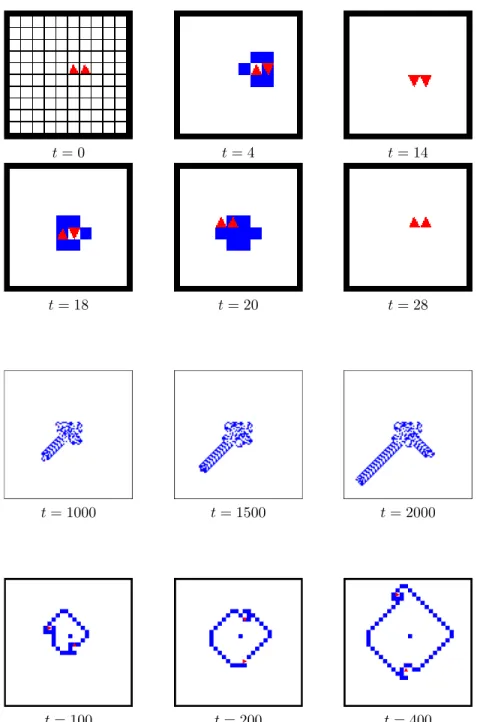
Let us first observe a simple evolution of a two-agent system where the two Turmites are placed next to each other with the same orientation: (0, 0, North) and (1, 0, North). This initial configuration illustrates how the choice of an update leads to different evolutions:
• Figure 4-top presents the evolution of the < Model 1, Allow > sys-tem. This systems has a cyclic behaviour: the system returns to its initial state in 28 steps. Similar cyclic behaviours were also observed in the synchronous multi-Turmite model considered by Chopard and Droz [5] and in the sequential system considered by Beuret and Tom-massini [2]. An open question is to know under which conditions cyclic patterns appear.
• Figure 4-middle presents the evolution of the system < Model 1, Exclude >. The behaviour is more “common” since the two Tur-mites escape to infinity by building two paths in different directions (this path-building behaviour was also observed in the three evo-lutions in Figure 3). The first Turmite starts building its path at t ∼ 400 and the second Turmite reaches the path-building behaviour at t ∼ 1700.
• Finally, Figure 4-bottom presents the evolution of the system < Model 2, Exclude >. We observe that the two Turmites follow each other’s path but with a difference of one cell (at the right of the previous path). This results in the apparition of a square constituted of cells
t= 0 t= 4 t= 14
t= 18 t= 20 t= 28
t= 1000 t= 1500 t= 2000
t= 100 t= 200 t= 400
Figure 4: Evolution of two Turmites starting from initial condition (0, 0, North) and (1, 0, North). (Top) < Model 1, Allow >, cyclic behaviour. (Middle) <Model 1, Exclude >, pathway building. (Bottom) < Model 2, Exclude >, ever-growing square.
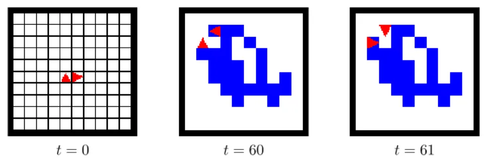
t= 0 t= 60 t= 61
Figure 5: Evolution of two Turmites starting from initial condition (0, 0, North) and (1, 0, East), < Model 1, Exclude > system. The system reaches a deadlock at time t = 60. The configuration at time t = 62 is identical to time t = 60.
in state 1, this square grows for ever, its width is increased by one at each of the Turmite’s return. Such behaviour was already observed by Langton, for whom they were a good a example of a “collabo-ration” between Turmites to build patterns. It is an open question to know whether more elaborate patterns can be built with similar cases of “collaboration”.
7.2
Deadlocks
Figure 5 shows the < Model 1, Exclude > system. The two Turmites are again put next to each other, but with the second Turmite turned by 90 degrees: (0, 0, North) and (1, 0, East). We observe that after 60 steps the system reaches a configuration where the two agents will not move. At time t = 60, the agents attempt to move to the same cell, as they turn and flip their cell. At time t = 61, they turn simultaneously and flip their cell. Again, their attempt to move to the same cell is blocked. As consequence, the configuration reached at time t = 62 is identical to the configuration at time t = 60 and the evolution is then cyclic with two static Turmites and two “blinking” cells. We call deadlocks the configurations where the Turmites are static. It is to our knowledge the first time that these phenomena are observed; their very existence is due to the synchronous updating of the system and to the introduction of the Exclude policy.
7.3
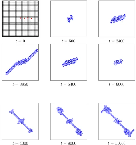
Path Retraction and Path Turn
Figure 6 shows a curious evolution of the < Model 1, Allow > system: two symmetric paths develop and retract cyclically. This phenomenon is obtained with four Turmites initially placed on a horizontal line, at distance 3 from each other, with alternating orientations. The cycle has length 6576 and can be decomposed into five parts: (a) from time t = 0 to time t = 1182, the system evolves in the “chaotic” regime, the pattern of 1-cells extends and then shrinks until the space is all-0 (the Turmites are in different positions than at t = 0); (b) from time t = 1183 to time t ∼ 2400 a new chaotic regime is started; (c) at time t ∼ 2400 two Turmites start
t= 0 t= 500 t= 2400
t= 3850 t= 5400 t= 6000
t= 4000 t= 8000 t= 11000
Figure 6: Initial condition is: (0, 0, North), (3, 0, South), (6, 0, North), (9, 0, South). (Top) < Model 1, Allow >, cyclic retracting path phenomenon. (Bottom) < Model 1 , Exclude >, turning path phenomenon.
building a pathway, (d) they are then rejoined by the two other Turmites and they interact at time t ∼ 3850; (e) the result of this interaction is to create a path retraction and the erasing of the 1-pattern until the initial condition is attained at time t = 6576.
This observation shows that paths can be retracted during their con-struction when two Turmites interact. Moreover, it appears that this path retraction is a particular case of a “pattern erasing regime” where the past actions of the Turmites are reversed. It is an open problem to analyse un-der which conditions this pattern erasing regime appears. An explanation of this phenomenon as a time-reversal symmetry is given by Chopard and Droz in [5]. From the first observations conducted, it seems that it is a consequence of a “collision” between two Turmites.
Interestingly, starting from the same initial condition with the Exclude policy leads to observe a “turning path” phenomenon (see Fig. 6-bottom. This phenomenon is obtained in five phases: (a) The four paths evolve in a chaotic regime; (b) Two Turmites T1, T2 build a path while the two
others T3 and T4 stay in a chaotic regime; (c) T3 and T4 enter into the
path built by T1, T2 and follow this path until they “collide” with T1, T2;
(d) This collision initiates a new chaotic phase with the four Turmites; (e) A new pair of Turmites emerges T′
1 and T2′ from the chaotic regime and
builds a path that is here orthogonal to the first path.
7.4
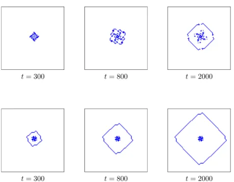
Ever-Growing Squares with Opposite
Rotat-ing Directions
Figure 7 presents an example where the same initial condition leads to the formation of ever-growing squares, but with squares growing in opposite directions. Both models are run with the Exclude policy, < Model 1, Exclude > gives birth to a square which grows with Turmites rotating counter-clockwise while the Turmites of < Model 2, Exclude > turn clock-wise. We also observe that that the transient phase before starting build-ing the square is shorter for Model 2 than for Model 1.
This indicates that is no general law of “conservation of momentum” in the multi-Turmite system. However, in some restricted cases, other conservation laws exist. For example, with the Allow policy, the fact that position and the orientation of the Turmites changes at each time step implies that parity conservation laws can be derived rather easily.
7.5
Gliders
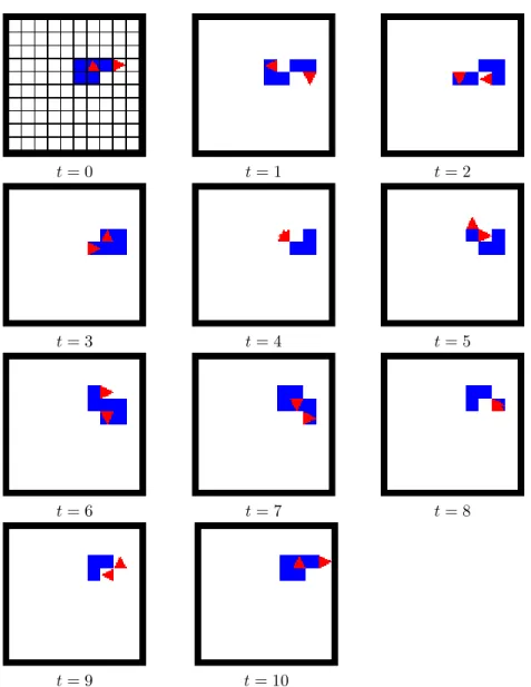
Last, but not least we report the observation of a new kind of translating pattern which we name “gliders” by analogy with cellular automata. Con-trarily to many cellular automata, like the game of Life, the apparition of gliders with in the multi-Turmite model is rare. We could observe only one configuration which gave birth to gliders and this configuration was found by chance out of dozens of experiments.
Figure 8 shows the evolution with a simple initial condition with four Turmites disposed in a square pattern. Note that the orientation of the Turmites is such that the initial condition is symmetric with respect to the central symmetry but it is not rotationally symmetric. The system evolves
t= 300 t= 800 t= 2000
t= 300 t= 800 t= 2000
Figure 7: Evolutions of two systems with initial condition: (0, 0, North), (0, 4, East), (4, 4, South), (4, 0, West). (Top) < Model 1, Exclude >, ever-growing square rotating counter-clockwise. (Bottom) < Model 2, Exclude >, ever-growing square rotating clockwise.
t= 0 t= 600 t= 640
Figure 8: Evolution of < Model 1, Allow > system with initial condition: (0, 0, East), (0, 4, North), (4, 4, West), (4, 0, South). Two gliders are ejected in diagonal directions.
t= 0 t= 1 t= 2
t= 3 t= 4 t= 5
t= 6 t= 7 t= 8
t= 9 t= 10
Figure 9: Focus on the translation cycle of a glider observed with the < Model 1, Allow>system.
chaotically until two gliders are “ejected” from the the central pattern at time t ∼ 550. Figure 9 shows a close-up on the translation mechanism of a glider: it is constituted of a pair of Turmites, which translate by (±1, ±1) every 10 time steps.
An interesting question is to know whether it is possible to take gliders as a basis for building a universal Turing machine with the multi-Turmite model. This is one of the numerous questions that remain to examine in order to have a more comprehensive view of the multi-Turmite model.
8
Discussion and Perspectives
Synthesis This article aimed at presenting fundamental tools for the mathematical definition of situated and reactive multi-agent systems. Fol-lowing the path drawn by Ferber and M¨uller [12], we exposed the thesis that multi-agent systems gain to be described as discrete dynamical sys-tems. The method we proposed to produce this description separates into two distinct parts what regards the description of the agents and their environment, on one side, and what regards the interaction between com-ponents, on the other side. We advocated that following the six steps of the method should bring the following effects:
• Defining multi-agent systems in a mathematical language allows us to clarify the hidden assumptions on how the components of a system should interact. Obviously, expressing multi-agent systems in this formalism necessitates some efforts, but among the positive counter-parts, we expect to ease the reproduction of the experiments. This point is important since reproducibility of experiments is a funda-mental requirement of scientific investigation. Another important point is to allow an expression of a synchronous updating of a multi-agent system: the synchronous updating scheme has the advantage of removing the artificial biases that may arise with an ad hoc choice of an updating order.
• Our method is also meant to evaluate to which extent a model is ro-bust to changes of its simulation scheme. Simulation schemes were defined as a combination of different possibilities of updating the system and solving conflicts. In the simple examples we studied, the conflicts were created by simultaneous attempts to move to a cell or to modify the cell state. More complicated models should gener-ate an even wider range of simulation schemes. Ideally, simulation programs should allow their users to define the agents’ behaviour in a first step and then to test different simulation schemes for each agent’s definition.
This mathematical approach to multi-agent systems is clearly limited to simple systems and even for such systems, limits have still to be pre-cised in many ways. We do not claim that our proposition fits all the scientific purposes and nor that it could be used to describe all the sys-tems. As a next step, its relevance should be to assessed by considering a wider range of examples. We see three main directions to follow this exploration: exploring further the multi-Turmite model or other related
models, searching for other expressions of the formalism, working on suit-able implementations of the formalism. Let us now conclude by describing briefly each of these three directions.
On the exploration of simple models The series of experiments we conducted allowed us to see that one single model, here the multi-Turmite model, may be defined differently, depending on what interpre-tation is chosen on its internal and observable states. The experiments we conducted with each model allowed us to reproduce previous observations as well as to discover new qualitative behaviours such as deadlocks and gliders. As these experiments are described using a rigorous and unam-biguous formalism, they can be reproduced and further investigations can be undertaken.
Simulation schemes were defined as a combination of the updating scheme and the influence management policies, which were themselves decomposed into many parts. The breaking of simulation scheme into elementary components facilitates the study of the role that plays each component in the global system’s behaviour. In this article, we focused our attention on displaying cases of non-robustness. However, the con-verse problem is also interesting: in which cases does the system behave robustly to the modifications of its simulation scheme? Our point is that if we consider natural models, such as real ants models, it may be well that the multi-Turmite system is rather an exception than a representa-tive example. It is probable that the robustness of the natural systems should somehow be translated into the models themselves and that small modification of the simulation scheme of the model should not trigger qualitative modifications of their behaviour.
On the formalism The formalism proposed in this article, although rigorous, should not be considered as a fixed and rigid proposition. In-stead, we emphasise that there are many directions in which it can be extended, either by broadening the abilities of the agents (direct commu-nication, birth and death of agents, continuous positions, etc.) or, on the contrary by narrowing the language to allow for a more “secure” descrip-tion. For example, no specification on the set of influences were given, which authorises arbitrary communications between agents or arbitrary interactions between agents and their environment. A possibility to pre-vent such effects, if they are unwanted, is to consider that influences are (a) “attached” to a cell and (b) act on cells which update their state ac-cording to a particular “cellular automaton rule”. This particular rule would take into account not only the state of the neighbouring cells but also the presence or absence of influences.
On the implementation The question of the actual coding of the formalism in a programming language was purposely left apart. Al-though there are certainly many programming techniques that sponta-neously come to mind, we underscore that an advantage of describing multi-agents systems as dynamical systems is to make them independent for any hardware or software contingencies. Of course much efforts remain
to be produced, for each class of model, and for each type of hardware and software, to identify what is the suitable coding technique to use. For example, we can remark that coding the Turmites on a sequential machine or on massively parallel computing device will not result in using the same structure. In the first case agents should be declared in an independent list while in the second case, they should rather be an attribute of the cell itself [17].
These are just a few directions open for further research and there are just as much remaining to tackle the question of determining, in the computer science modelling area, what part of an observation is due the model and what part is due to the simulation scheme.
References
[1] Robert L. Axtell, Effects of interaction topology and activation regime in several multi-agent systems, Multi-Agent-Based Simulation, Lec-ture Notes in AI Volume 1979, Springer-Verlag, 2001, pp. 33–48. [2] Olivier Beuret and Marco Tomassini, Behaviour of multiple
gener-alized langton’s ants, Proceeding of the Artificial Life V Conference (Nava, Japan) (C. Langton and K. Shimohara, eds.), MIT Press, 1998, pp. 45–50.
[3] Leonid A. Bunimovich and Serge E. Troubetzkoy, Recurrence prop-erties of lorentz lattice gas cellular automata, Journal of Statistical Physics 67 (1992), 289–302.
[4] Geoffrey Caron-Lormier, Roger W. Humphry, David A. Bohan, Cathy Hawes, and Pernille Thorbek, Asynchronous and synchronous updating in individual-based models, Ecological Modelling 212 (2008), no. 3-4, 522–527.
[5] Bastien Chopard and Michel Droz, Cellular automata modeling of physical systems, Cambridge University Press, 1998.
[6] David Cornforth, David G. Green, and David Newth, Ordered asyn-chronous processes in multi-agent systems, Physica D: Nonlinear Phe-nomena 204 (2005), no. 1-2, 70–82.
[7] Alexander K. Dewdney, Two-dimensional Turing machines and tur-mites make tracks on a plane, computer recreations, Scientific Amer-ican (1989), 180–182.
[8] Nazim Fat`es, Fiatlux CA simulator in Java, See http://webloria. loria.fr/∼fates/.
[9] , Asynchronism induces second order phase transitions in el-ementary cellular automata, Journal of Cellular Automata 4 (2009), no. 1, 21–38, http://hal.inria.fr/inria-00138051.
[10] Nazim Fat`es and Michel Morvan, An experimental study of robustness to asynchronism for elementary cellular automata, Complex Systems 16 (2005), 1–27.
[11] Nazim Fat`es, Michel Morvan, Nicolas Schabanel, and Eric Thierry, Fully asynchronous behavior of double-quiescent elementary cellular automata, Theoretical Computer Science 362 (2006), 1–16.
[12] J. Ferber and J.P. M¨uller, Influences and reaction : a model of situ-ated multiagent systems, Proceedings of the 2nd International Con-ference on Multi-agent Systems, 1996, pp. 72–79.
[13] Anah´ı Gajardo and Eric Goles, Dynamics of a class of ants on a one-dimensional lattice, Theoretical Computer Science 322 (2004), no. 2, 267–283.
[14] Alexander Helleboogh, Giuseppe Vizzari, Adelinde Uhrmacher, and Fabien Michel, Modeling dynamic environments in multi-agent sim-ulation, Autonomous Agents and Multi-Agent Systems 14 (2007), no. 1, 87–116.
[15] Christopher G. Langton, Studying artificial life with cellular au-tomata, Physica D 22 (1861), 120–149.
[16] Fabien Michel, The IRM4S model: the influence/reaction princi-ple for multiagent based simulation, AAMAS’07, Sixth International Joint Conference on Autonomous Agents and Multiagent Systems, Honolulu, Hawaii, USA, May 14-18, 2007.
[17] Antoine Spicher, Nazim Fat`es, and Olivier Simonin, From reactive multi-agent models to cellular automata - illustration on a diffusion-limited aggregation mode, Proceedings of ICAART’09 (to appear), Lecture Notes in Computer Science, Springer, 2008, http://hal. archives-ouvertes.fr/hal-00319471/.
[18] Giuseppe Vizzari and Stefania Bandini, Coordinating change of agents’ states in situated agents models, AAMAS ’05: Proceedings of the fourth international joint conference on Autonomous agents and multiagent systems (New York, NY, USA), ACM, 2005, pp. 1319– 1320.
[19] Gerhard Weiss, Multiagent systems a modern approach to distributed artificial intelligence, ISBN 978-0-262-73131-7, MIT Press, 1999. [20] Danny Weyns and Tom Holvoet, Model for simultaneous actions in
situated multi-agent systems, MATES, Lecture Notes in Computer Science, vol. 2831, Springer, 2003, pp. 105–118.
[21] Michael Wooldridge, An introduction to multiagent systems, ISBN 0 47149691X, John Wiley and Sons (Chichester, England), 2002.
9
Annex
In order to ease the reading of the paper, we have placed here two mathe-matical definitions: the asynchronous updating of the system and the ho-mogeneity of the agents of a system. Defining the asynchronous updating is important since it is the updating method that is the most commonly used with multi-agents. As for the homogeneity, it is a property that is often required in the design of emergent systems: one often wants to observe the emergence of a global interesting behaviour even with sim-ple and equal agents (e.g., there is no chief agent that realises a central coordination of the other agents).
9.1
Asynchronous Updating of Systems
To express the asynchronous updating of the system, we keep the same Evolve function, but going from time t to t + 1 requires a sequence of computations. As a starting point, let us examine how to define a sequen-tial updating in a fixed order, say from agent 1 to agent A. The first agent makes its perception, it produces its influence, this influence is taken into account to modify the environment, its position and state and, possibly, it may also modify the position and state of the other agent (for example if an agent releases a “push” influence on a neighbouring agent). Then, the second agent perceives the new state of the environment, and performs the same type of actions. We thus need to compute intermediary states of the environment and of the agents: we introduce the notation t + k.∆t where ∆t = 1/A denotes an intermediary step. At each step k ∈ {1, . . . , A}, the “active” agent has index k and its perception function is now given by:
πk(t) = Perceivekˆ (~e, ~p, ~o)(t + (k − 1)∆t) ˜
The definitions of each influence and each new internal state are not mod-ified: γk(t) = Decidekˆ ik(t), πk(t) ˜ and ik(t + 1) = AgentUpdatekˆ ik(t), πk(t) ˜
However, the global collection of influences at “time” t + (k − 1)∆t has now to be defined as a vector all composed of empty influences except at rank k: ~γ` t + (k − 1)∆t ´ = (⊙, ⊙, . . . , γk(t), , . . . , ⊙).
The intermediary states of the environment and the agents are given by:
(~e, ~p, ~o)(t + k∆t) = Evolveˆ (~e, ~p, ~o, ~γ)(t + (k − 1)∆t) ˜
The state at time t + 1 is obtained for k = A, i.e., when the system has completely updated its state. It is easy to generalise this definition to other type of asynchronous updating, for example by considering that the order of updating is modified at each time step (i.e., after updating all the agents) or by considering an α-asynchronous updating where the agents have a probability α to be updated [10].
9.2
Homogeneity of Agents
Informally, we say that we have a homogeneous system in the case where all agents have the “same” perception, decision and internal state updat-ing functions. To express formally the condition that agents have the “same” perception, note that, as the perception naturally depends on the position of the agent pa, and thus on its index a we cannot simply say
that the perception does not depend on a. Intuitively, we say that the agents have the “same perception” if for a given agent, any other agent would have the same perception if it were placed at the same position. To express the two other conditions is easier we only need to verify that Decideaand AgentUpdatea are independent from a.
Formally, we say that the system is homogeneous iff for any pair of agents x and y in {1, . . . , A}:
∀(~e, ~p1, ~o1), Perceivex(~e, ~p1, ~o1) = Perceivey(~e, ~p2, ~o2) and
Decidex= Decideyand
AgentUpdatex= AgentUpdatey
where (~p2, ~o2) is obtained by a permutation of (~p1, ~o1) at the indexes x
and y. As an example of a non-homogeneous system, consider the case where agent 1 perceives only the state of the cell on which it is located and where agent 2 perceives the state of the cell situated north of it. This would translate into:
Perceive1(~e, ~p, ~o) = ep
1
Perceive2(~e, ~p, ~o) = ep2+(0,1)
It is easy to verify that this system is not homogeneous. The multi-Turmite system that we consider is homogeneous.