HAL Id: insu-01472195
https://hal-insu.archives-ouvertes.fr/insu-01472195
Preprint submitted on 20 Feb 2017
HAL is a multi-disciplinary open access archive for the deposit and dissemination of sci-entific research documents, whether they are pub-lished or not. The documents may come from teaching and research institutions in France or abroad, or from public or private research centers.
L’archive ouverte pluridisciplinaire HAL, est destinée au dépôt et à la diffusion de documents scientifiques de niveau recherche, publiés ou non, émanant des établissements d’enseignement et de recherche français ou étrangers, des laboratoires publics ou privés.
Distributed under a Creative Commons Attribution - NonCommercial - ShareAlike| 4.0
Rupture process of the Oklahoma Mw5.7 Pawnee
earthquake from Sentinel-1 InSAR and seismological
data
Raphaël Grandin, Martin Vallée, Robin Lacassin
To cite this version:
Raphaël Grandin, Martin Vallée, Robin Lacassin. Rupture process of the Oklahoma Mw5.7 Pawnee earthquake from Sentinel-1 InSAR and seismological data. 2017. �insu-01472195�
Rupture process of the Oklahoma Mw5.7 Pawnee earthquake
from Sentinel-1 InSAR and seismological data
Raphaël GRANDIN,1* Martin VALLÉE,1 Robin LACASSIN1
1 Institut de Physique du Globe de Paris (IPGP), UMR 7154, Sorbonne Paris Cité, Université Paris Diderot, Paris, France.
grandin@ipgp.fr ; vallee@ipgp.fr ; lacassin@ipgp.fr
* To whom correspondence should be addressed; Email: grandin@ipgp.fr
Abstract
Since 2009, Oklahoma has experienced a sore in induced seismicity, a side effect of extensive saltwater injection into subsurface sedimentary rocks. The seismic hazard entailed by these regional-scale injection operations is however difficult to assess. The September 3, 2016, Mw5.7 Pawnee earthquake is the largest since the increase of seismic activity. The event was preceded by a mb3.2 foreshock two days before, and changes in injection rates have been reported on wastewater disposal wells located less than 10km from the epicenter, suggesting that the earthquake may have been induced. Using Sentinel-1 spaceborne interferometric synthetic aperture radar, we unambiguously show that the earthquake produced peak-to-peak line-of-sight displacement of 3 cm at the surface. Kinematic inversion of geodetic and seismological data shows that the main seismic rupture occurred between 4 and 9km depth, over a length of 8km, with slip reaching at least 40cm. The causative fault is entirely buried within the Precambrian basement, i.e. well beneath the Paleozoic sedimentary pile where injection is taking place. Potentially seismogenic faults in the basement of Oklahoma being poorly known, the risk of Mw≥6 events triggered by fluid injection remains an open question.
INTRODUCTION
Central US, and in particular the state of Oklahoma, has experienced a marked increase in seismicity rate since 2009 (Ellsworth, 2013; Hough and Page, 2015; Frohlich et al., 2016). A body of evidence, the most compelling being the temporal and spatial coincidence (Fig. 1a), strongly suggests that this enhanced seismic activity is primarily induced by the injection of large volumes of wastewater into porous sedimentary formations (Walsh and Zoback, 2015; Weigarten et al., 2015). Injected wastewater consists of variable proportions of coproduced water naturally present in the reservoir and coming with oil and gas, as well as of flow-back of fluids previously injected in the reservoir for enhanced recovery, or fracking (e.g. Rubinstein and Mahani, 2015). As oil and gas exploitation in continental US has boomed in the last decade, the amount of produced wastewater followed the same trend.
The issue is particularly acute in Oklahoma because wastewater is being injected on a regional scale. The necessity of disposing of enormous volumes of wastewater arises from an exceptionally high volume ratio of produced saltwater:fossil fuel, as large as 7 to 9 in some parts of Oklahoma, as opposed to 1 or less in other regions (Murray, 2014). Such a high ratio originates from increasing exploitation of unconventional reservoirs by stimulated production techniques (Matson, 2013; Murray, 2015; Rubinstein and Mahani, 2015). The bulk of the coproduced saltwater is mainly injected into the Arbuckle group, which consists of u n d e r p r e s s u r e d O r d o v i c i a n - C a m b r i a n limestones and dolomites (Murray, 2015). These formations are located at the very bottom of the sedimentary pile, just above contact with the crystalline basement.
The dramatic increase in the number of felt earthquakes has raised legitimate concern about the possibility of triggering even larger earthquakes. To help answer this pressing issue, studying past and present seismic activities in this previously seismically quiet intraplate
Figure 1. a. Class II wastewater disposal wells in the 2009-2016 period (squares) and seismicity with M>2.5 reported by USGS for the same period (circles). Mapped faults are shown in the background (Holland, 2015). Recent clusters of seismicity are indicated by stars. Fa : Fairview MWmax5.1 2016 (Yeck et al., 2016a); Mi : Milan MWmax4.9
2014 (Choy et al., 2016); Gu: Guthrie MWmax4.0 2014 (Benz
et al., 2015); Jo : Jones 2009-2014 (Keranen et al., 2014); Cu: Cushing MWmax4.3 2014 (McNamara et al., 2015) and
Mwmax5.0 2016; Pr: Prague MWmax5.7 2011 (Keranen et al.,
2013). b. Disposal wells in the area of the 2016 Pawnee earthquake (rectangle in a.) are indicated by squares scaled according to the average injection rate in the 2 months prior to the Pawnee mainshock. Solid circles are aftershocks of the Pawnee earthquake reported by Yeck et al. (2016b) scaled according to magnitude. Diamond indicates 1 September 2016 foreshock (Yeck et al., 2016b). Empty circles represent the USGS seismicity in the 2009-2016 period as in a.
region is an obvious need. Most of the well-recorded seismicity in the area lies within the Precambrian basement (Keranen et al., 2013, 2014; Choy et al., 2016; McNamara et al., 2015; Yeck et al., 2016a). This observation suggests that faults located at seismogenic depth (5-15km) could be destabilized by injection operations carried out in the shallow sub-surface. Unfortunately, due to lack of coseismic ground deformation measurements, rupture area of the largest recent earthquakes could not be easily determined. Hence, the actual radius of influence of injection operations, although suspected to be greater than 10 km horizontally and perhaps 5-10 km vertically (Yeck et al., 2016a; Keranen et al., 2013; Choy et al., 2016; Shirzaei et al., 2016), remains subject to uncertainty.
The 3 September 2016 Mw5.7 Pawnee earthquake is the largest reported earthquake in Oklahoma since the recent increase of seismicity. The earthquake reached shaking intensity VII, causing damage to some buildings in the epicentral area (USGS, 2015). The aftershock sequence of the Pawnee earthquake was precisely recorded thanks to rapid deployment of a seismic network (Yeck et al., 2016b). Aftershock seismicity is concentrated at ~6km depth, delineating an ESE-WNW trending vertical fault (Fig. 1b). However, the depth and slip area of the causative fault involved in mainshock remain poorly constrained.
Synthetic aperture radar interferometry (InSAR) has proved to be a powerful tool to characterize seismic and aseismic deformation induced by hydrologic effects of human activity (e.g. Barnhard et al., 2011; González et al., 2012; Yeck et al., 2016b). Yet, previous M>5 earthquakes in Oklahoma could not be studied by InSAR due to lack of sufficient observations. As a consequence, the combined effect of decorrelation and atmospheric noise
could not be overcome, explaining why these small events have remained, so far, undetectable from space. The new Sentinel-1 system of the European Space Agency (ESA), consisting of two twin satellites launched in April 2014 and April 2016, operating in a novel wide-swath acquisition mode, has recently allowed for significant improvements in terms of detection of small deformation signals (e.g. Geudtner et al., 2014). Due to the relatively strong magnitude of the Pawnee earthquake, the static coseismic surface displacement was deemed sufficient for a measurement using the Sentinel-1 system.
In the following, using this geodetic information together with seismic waves recorded at close and far distances, we analyze the spatio-temporal rupture process of this moderate earthquake. Its relationship with injection operations and implications in terms of seismic hazard are also discussed.
INSAR PROCESSING METHODS
In order to isolate the static surface deformation induced by the Pawnee earthquake, we collected data acquired by ESA's Sentinel-1 satellites before and after the earthquake, and computed a number of interferograms spanning different time intervals. We selected images from relative orbit 34, which provide the most complete temporal coverage (Fig. 2). They are acquired in ascending pass with an incidence angle of 41° in the epicentral area. An anomaly is indeed d e t e c t e d i n t h e e p i c e n t r a l a r e a f o r interferograms bracketing the earthquake. However, because of the small magnitude of the displacement (a few centimeters), individual interferograms are dominated by atmospheric turbulence (Yeck et al., 2016b). In order to improve the signal-to-noise ratio, we compute a time-series of the line-of-sight signal with a temporal resolution of 12 days. This fine temporal resolution, which is a uniquecapability of the Sentinel-1 system, makes it possible to isolate the subtle signal associated with the earthquake by averaging out non-t e m p o r a l l y c o r r e l a non-t e d a non-t m o s p h e r i c disturbances.
Sentinel-1 TOPS data is first pre-processed using the method described in Grandin, 2015. The NSBAS software (Doin et al., 2011), which partly relies on ROI_PAC (Rosen et al., 2004) for individual interferometric calculation, is then used for time-series processing. We use six images acquired prior to the mainshock, and six images acquired after. After co-registration onto a single master i m a g e ( 2 0 1 6 / 0 7 / 2 9 ) , a t o t a l o f 5 5 interferograms are computed (Fig. 2). The choice of the interferograms is based on a minimization of the perpendicular baseline and a minimum redundancy of 7 interferograms for any acquisition. Topography is removed using a 10 m resolution digital elevation model from the National Elevation Dataset (NED) (Gesch et al., 2002). To improve the signal-to-noise ratio, interferograms are then multi-looked by a
factor 128 in range and 32 in azimuth, leading to a ground posting of approximately 500 meters, and an adaptive filter is applied (Goldstein and Werner, 1998). Finally, unwrapping is performed using the branch-cut algorithm (Goldstein and Zebker, 1988).
Figure 2. Spatio-temporal relation between acquisitions used in this study. Vertexes represent Sentinel-1 acquisitions in a baseline-time diagram, whereas lines connecting the acquisitions correspond to computed interferograms. Thin grey lines indicate interferograms that were discarded due to poor quality. Sentinel-1A acquisitions correspond to circles, whereas the only Sentinel-1B acquisition is indicated by a square. Master image is indicated by a ticker symbol. Mainshock date is marked by vertical dashed line.
Figure 3. a. Line-of-sight cumulative interferometric signal as a function of time decomposed on each time interval separating two successive acquisitions. Interferograms are here unwrapped and re-wrapped with a color palette cycle of 2.5 cm for the purpose of facilitating interpretation. Dashed rectangle indicates epicentral region of the Pawnee earthquake. The six upper panels represent acquisitions preceding the earthquake, whereas the six lower panels are for acquisitions made after the earthquake. b. Line-of-sight displacement deduced from pixelwise inversion using a model consisting of a constant (A) and a step function (B) (Equation 1).
Using NSBAS software, a time-series is computed from the interferograms using a small-baseline approach, which consists in isolating the apparent line-of-sight signal corresponding to each time interval separating two consecutive acquisitions (e.g. Berardino et al., 2002; Schmidt and Bürgmann, 2003). Nine interferograms corrupted by large-scale unwrapping errors are first removed from the analysis. A first iteration is carried out to identify and correct small unwrapping errors, which are detected according to the pixelwise misclosure they provoke in the interferometric network (Cavalié et al., 2007; López-Quiroz et al., 2009). Pixels leading to a residual RMS misclosure exceeding 2.5 radian (equivalent to 1.1 cm) are rejected. This cutoff was chosen by trial and error to exclude points evidently corrupted by residual small-scale unwrapping errors.
Low pass temporal filtering is then applied in the time-series inversion to separate any
steadily accumulating signal (either due to deformation (e.g. Shirzaei et al., 2016) or seasonally-aliased atmospheric phenomena (e.g. Doin et al., 2009)) from the erratic contribution of atmospheric turbulence and earthquake signal. According to this test, no steady signal could be detected in the time-series, meaning that deformation can be entirely interpreted as coseismic, the remaining contribution to phase variations being temporally uncorrelated atmospheric turbulence. As a consequence, the low-pass filtering step is discarded in the following in order to avoid aliasing of the coseismic signal. A second iteration is performed by weighting interferograms by the inverse of the RMS residual in each time step. In a third iteration, another subset of two interferograms affected by large atmospheric noise, corresponding to the largest overall residual, are discarded. An unfiltered time-series inversion is finally performed using the 44 remaining interferograms (Fig. 3, top).
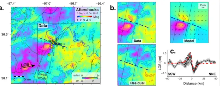
Figure 4. a. Ground deformation for the period spanning the Pawnee mainshock derived from Sentinel-1 radar interferometry (InSAR). Background shows motion in the line-of-sight (LOS) of the satellite using a color palette cycle of 2.5cm. Positive is for motion away from the satellite. Negative is for motion toward the satellite. The LOS direction is indicated by the arrow at the bottom left. Dashed line marks the surface projection of the upper edge of the modeled fault. Circles and lines are aftershocks and faults, respectively, as in Fig. 1. b. Zoom in the epicentral area (highlighted by rectangle in a.) showing observed, modeled and residual displacement. The model is here computed from the kinematic slip model, deduced from joint inversion of geodetic and seismological data. Arrows indicate predicted horizontal components of surface displacement. c. Comparison of observed and synthetic LOS displacement along swath profile indicated by the thin dotted lines in a. and b. The thin continuous line is the observed displacement averaged in 0.5-km bins in a 10km-wide swath profile, with the grey band in the background indicating the data range in the swath profile. Circles show decimated data used as input for the inversion and associated error bars. Thick dashed line is synthetic displacement from finite source kinematic inversion sampled in the middle of the swath profile.
At this stage, the phase changes corresponding to each time interval separating consecutive acquisitions are determined. They include both the atmospheric fluctuations and the coseismic earthquake signal. In order to isolate the contribution of the Pawnee mainshock, we use a simple forward model consisting of the sum of a constant term A (corresponding to atmospheric noise in the reference image) and a step function H with amplitude B (the earthquake signal), synchronized with the date of the earthquake tEQ :
A +H(tEQ)xB (1)
Misfits between observation and model are interpreted as reflecting atmospheric artifacts. Using the forward model d=Gm, where d is the data column vector, m is the column vector of model parameters and G is the design matrix containing ones and zeros, corresponding to the discretization of Equation (1), the weighted least-squares problem is solved as :
m' = (Gt W G )-1 Gt W d (2)
Weights in W are determined by assessing the level of noise in the maps of incremental deformation from each time interval. This is achieved by computing empirical semi-variograms clipped to a maximum distance x of 75 km (after masking out the deformation area), and fitted with an exponential model with expression S2*[1-exp(-x/r)] + n. We use
the asymptotic semi-variance in the exponential model Si2 to quantify the uncertainty associated
with each time step interferogram i. These values are then used to fill a weight matrix
W=diag(1/Si2) used to solve the pixelwise
weighted least-squares problem.
Finally, the time-series interferograms are geocoded and subsampled based on model resolution (Lohman and Simons, 2005), with a minimum spacing of 2km between data points in the near field (i.e. approximately within 15km of fault trace, see Fig. 4c).
We find that the earthquake is responsible for two areas of significant line-of-sight motion, taking the form of two distinct lobes characteristic of a blind strike-slip fault (Fig. 4a). The location of the fringes, to the west of the epicenter, is consistent with this displacement being induced by a combination of east-west and vertical motion. Peak-to-peak amplitude of line-of-sight displacement reaches 3cm over a distance of 10km. The shape and magnitude of this fringe pattern provide strong constraints on the location and depth of the rupture area. Other features visible in the coseismic interferogram (Fig. 3 and 4) likely reflect residual atmospheric artifacts with maximum amplitude of ~1.5cm.
SEISMOLOGICAL DATA AND
VELOCITY MODEL
The earthquake has been recorded by local broadband seismometers from GS, N4, TA, and OK networks. Even if some of the closest stations are clipped, the subset of five stations shown in Figure 5a offers a good azimuthal coverage of the earthquake. We first conduct a point source inversion of these data, in order to determine the first-order characteristics of the earthquake (focal mechanism, centroid depth) together with a suitable structure model. The method used, hereafter referred as MECAVEL, s i m u l t a n e o u s l y o p t i m i z e s ( w i t h t h e Neighborhood Algorithm of Sambridge, 1999) the source parameters and a simplified velocity model, parametrized by a superficial low-velocity layer above a crustal increasing gradient. The searched source parameters include the strike, dip, and rake of the focal mechanism, the centroid location, the source origin time and duration, and the moment magnitude. Waveform modeling in the 1D velocity model is performed with the discrete wave number method of Bouchon (1981). In the MECAVEL method, the three-component
displacement waveforms are bandpassed between a low frequency (Fc1) and a high
frequency (Fc2) threshold. Fc1 is typically
chosen above the low-frequency noise that may affect the waveforms of a moderate earthquake and Fc2 is mostly controlled by the limited
ability of a 1D model for the waveform modeling. Fc2 has also to be chosen below the
earthquake corner frequency, as the earthquake time history is simply modeled by a triangular source time function. In the specific case of the Pawnee earthquake, Fc1 is chosen at 0.02Hz
(classical value for a moderate earthquake) and Fc2 at 0.125Hz; the latter value can here be
chosen higher than in more complex media (for example in subduction zones), which enlarges the frequency range and hence the parameter resolution. Another application of the MECAVEL method in a different context can be found in Mercier de Lépinay et al. (2011), where the aftershocks of the 2010 Haiti earthquake are analyzed.
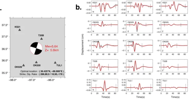
We show in Fig. 5a the optimal source parameters determined by the MECAVEL method and the associated waveform agreement in Fig. 5b. We find that the focal
mechanism of the Pawnee earthquake is consistent with nearly pure left-lateral strike-slip on an ESE-WNW trending vertical fault, in agreement with the alignment of aftershocks reported by Yeck et al., 2016a (Fig. 1). The epicentral centroid location, shifted about 2km in the East direction compared to the USGS epicenter, also favors the activation of the plane delineated by aftershocks. The centroid depth is constrained at 5.6 km, i.e. well within the Precambrian basement. Fig. 6b shows the optimized velocity model which scope is to represent an equivalent propagation medium, possibly not directly interpretable in terms of real structure. We however note that the inverted thickness of the shallow layer (about 2km) agrees well with the information available for the basement depth in the epicentral area (Fig. 6a) (Campbell and Weber, 2006).
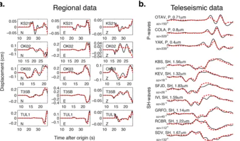
More precise analyses of the Pawnee earthquake (see next section) require to model the waveforms at higher frequency. To do so, we consider the local displacement waveforms in the frequency range [0.02Hz 0.5Hz] and restrain our analysis to the early part of the seismograms, comprised between the first
P-Figure 5. Point source inversion a. Local stations (triangles) and optimal source parameters from MECAVEL point source inversion. Note that the moment magnitude is found slightly larger (5.71) in the finite fault inversion. b. Comparison between observed (thin continuous line) and modeled (thick dashed line) three-component (N,E,Z) seismograms for the point source inversion. Here, data and synthetics are filtered between 0.02Hz and 0.125Hz.
wave arrival and a few seconds after the S-wave arrival (Fig. 7b). This excludes the high-frequency surface-waves, which carry more information about unknown characteristics of the propagation medium than on the source. We also include body-wave records at teleseismic distances f r o m t h e F e d e r a t i o n o f D i g i t a l Seismograph Networks (IRIS-USGS and GEOSCOPE networks), band-pass filtered in displacement between 0.0125Hz and 0.5Hz. Three P-wave and seven SH-wave records with good signal-to-noise ratio in this frequency range are selected (Fig. 7a).
KINEMATIC SLIP INVERSION
The geodetic and seismic data are jointly inverted using the method of Delouis et al., 2002 (see also Delouis et al., 2010 and Grandin et al., 2015), adapted here for a m o d e r a t e m a g n i t u d e e a r t h q u a k e configuration. The modeled fault is subdivided into 9 columns along strike and 7 rows along dip, measuring 1.5 km along strike and dip. The geometry is held fixed according to parameters determined from the point source inversion (strike = 288°, dip = 88°). Fault location is determined by fixing one grid node to the coordinates of the USGS epicenter (36.425°N, 96.929°W, depth = 5.6km). Sub-faults forming the upper and lower edges of the modeled finite fault are centered on depths of 2.6 km and 11.6 km, respectively. The waveforms are modeled by summing point sources located at the center of each subfault, with individual source time functions consisting of two isosceles triangular shaped functions with duration 1s. The onset time ofFigure 6. a. Depth to the basement in Oklahoma deduced from well data (Campbell and Weber, 2006). Area of Pawnee earthquake is indicated by the circle. Background is an interpolation of individual well data, indicated by dots.
b. Velocity model from MECAVEL point source inversion. Figure 7 (below). Finite source kinematic inversion a. Observed (thin continuous line) and modeled (tick dashed line) waveforms at local stations. Three-component (N,E,Z) displacement seismograms (filtered between 0.02Hz and 0.5Hz) are shown and modeled in a window starting from the P wave arrival and stopping a few seconds after the S-wave arrival. b. Observed (thin continuous line) and modeled (tick dashed line) waveforms at teleseismic distances. P-waves are shown in the three subplots at the top, and SH waves on next seven subplots below, both being bandpass filtered in displacement between 0.0125Hz and 0.5Hz. Duration shown is 21s and 30s for P- ans SH-waves, respectively. Name, azimuth of the station (az) and maximum amplitude in microns are indicated for each seismogram.
slip, together with the rake angle and slip amount of individual point source, are determined by a simulated annealing optimization algorithm. The onset time of slip is constrained by average rupture velocities allowed to vary between 0.5km/s and 3km/s and the rake angle is constrained to remain at +/-15° from the pure strike slip mechanism determined in the MECAVEL inversion. The cost function to be minimized includes the average of the root-mean-square misfit of each data set (InSAR, regional data, teleseismic data) as well as the spatial and temporal roughness of coseismic slip, rupture velocities and rake angle variations. All synthetics are computed in the velocity model optimized in the previous section through the MECAVEL point-source approach (Fig. 6b). Specifically, local synthetic seismograms and teleseismic P and SH displacements are computed using the discrete wave number method of Bouchon (1981) (Bouchon, 1981) and the reciprocity approach of Bouchon (1976) (Bouchon, 1976), respectively. Static displacements for InSAR are computed using the static Green functions approach of Wang et al., 2003.
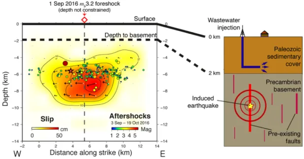
The space-time evolution of slip determined by the joint inversion of InSAR, local and teleseismic seismological data, is shown in Fig. 8 a n d 9 . T h e s e i s m i c m o m e n t o f Mo=4.64x10¹⁷N.m (Mw=5.71), slightly larger
than in the MECAVEL point-source inversion, is released in 4 seconds (Fig. 8). We find slip to be concentrated in a 8km long rupture area, at depths comprised between 4 and 9km, over which the slip reaches at least 40cm (Fig. 9). The aftershocks of the Pawnee earthquake appear to delineate the upper edge of the main slip area (Fig. 9). Significant slip (>10cm) at shallow depth is excluded thanks to the high model resolution in the 0-4km depth range provided by InSAR data. After a slow start in the hypocentral area during the first second, the rupture propagates both eastward (in agreement with the location of the MECAVEL centroid) and downward (Fig. 8). The rupture remains therefore entirely confined within the basement, failing to enter the superficial sedimentary cover. These first-order features remain valid when using the hypocenter depth of 4.7km reported by Yeck et al. (2016b), albeit at the cost of a slightly degraded fit and increased space-time complexity of the source.
DISCUSSION AND CONCLUSIONS
Although it is generally difficult to ascertain the causal relationship between wastewater injection and the occurrence of a particular earthquake, the context strongly suggests that the 2016 Pawnee earthquake represents another case of induced seismicity (Fig. 10). Indeed, in the year preceding the mainshock, at least twoFigure 8 a. Time of peak slip rate release referenced to the hypocentral time for the area of significant slip. Star marks hypocenter location. b. Source time function derived from the kinematic slip inversion.
wells were injecting saltwater at rates exceeding 500m3/day within 7km of the
e p i c e n t e r ( w e l l s “ O L D H A M ” a n d “SCROGGINS”) (Fig. 10a and 10b). Furthermore, an increase of the injection rate is reported at two wells located near the epicenter o f t h e P a w n e e e a r t h q u a k e . A t w e l l “SCROGGINS” (7km), injection rate increased by more than 50% in the three months prior to the earthquake, reaching a peak of 1100m3/day
in early August 2016 (Fig. 10c). It may be argued that these changes could have destabilized the fault involved in the Pawnee sequence, as changes in injection rates with the same order of magnitude and taking place over similar distance and duration were reported before the nearby Cushing and Milan seismic sequences (Choy et al., 2016; McNamara et al., 2015).
On a shorter time scale, even more rapid changes in injection rate can be noticed. At well “NORMAN” (8km), in spite of a significantly lower average injection rate of only 35m3/day in the two months preceding the
Pawnee earthquake, the injection rate was abruptly increased by a factor 6 on 28 August
2016, i.e. five days before the mainshock (Fig. 10d). According to Yeck et al. (2016b), a mb3.2 foreshock was recorded in the epicentral area of the Pawnee earthquake on 1 September 2016 (diamond in Fig. 1, 9 and 10). Retrospective analysis of microseismicity in the epicentral area of the Pawnee earthquake revealed that this foreshock belonged to an episode of enhanced seismicity that had started 90 days before the mainshock (Walter et al., 2017). Should the hypothesis of an injection-induced earthquake hold for the 3 September Pawnee mainshock, then these foreshocks may represent a case of precursory seismic activity. However, in spite of the spatial and temporal coincidence between seismic activity and changes injection rates in the Pawnee area, categorizing with certainty the Pawnee earthquake as an induced earthquake would require further investigation, in particular the careful validation of reports made by disposal well operators.
Our study reveals that nucleation of the 2016 Pawnee earthquake occurred deep into the basement, whose top lies at 2 km under the surface (Fig. 7). The earthquake may therefore result from destabilization of a fault buried 3-4
Figure 9. Slip model of the Pawnee earthquake from joint kinematic inversion of geodetic and seismological data. Aftershocks are from Yeck et al., 2016b. Diamond and vertical dashed line indicate 1 September 2016 foreshock (Yeck et al., 2016b). Basement depth is indicated by horizontal dashed line. Star marks hypocenter location.
km below the depth range where fluids are being injected. Similarly deep aftershocks were reported following the M5.7 2011 Prague (McNamara et al., 2015) and M5.1 2014 Fairview (Yeck et al., 2016a) earthquakes. Two physical mechanisms can explain this induced response: (a) pore pressure increase on the fault plane, and (b) remote stress triggering due to host rock poroelastic deformation (Ellsworth, 2013). While the latter mechanism decays rapidly over short ranges, the former is more problematic to quantify. Indeed, the presence of pervasive fracturing within the basement makes it possible for fluid pressure changes to be conveyed down to great depth (McGarr, 2014). This effect heavily distorts the shape of the perturbed volume of surrounding rocks away from the spherical shape predicted by a simple
isotropic theoretical model (Chang and Seagall, 2016). The resulting magnitude and location of fluid pressure perturbations are therefore subject to large uncertainties.
Whichever mechanism should apply, the link between the 2016 Pawnee earthquake and s h a l l o w i n j e c t i o n a c t i v i t i e s i s n o t straightforward. The rupture has nucleated well into the basement and coseismic slip seems to have died down as it propagated updip (Fig. 8). The rupture therefore failed to enter the superficial sedimentary layers that cover the basement, even though the effect of fluid injection would be expected to be highest at the shallow depths where injection is taking place. Instead, the Pawnee rupture activated a previously unmapped fault entirely confined
Figure 10. a. Location of main wastewater injection wells (inverted triangles) operating in the Pawnee area prior to the 3 September 2016 Mw5.7 Pawnee earthquake. Open circles are aftershocks from Yeck et al., 2016b. Diamond indicates 1 September 2016 foreshock (Yeck et al., 2016b). b. Daily injection rate averaged from 1 July to 3 September 2016 for wells indicated in a. c. Evolution of daily injection rates (squares) for three selected wells from 1 January 2015 to 1 November 2016. Circles show pressure data, when available. Date of Pawnee mainshock is indicated by the vertical dashed line. Inset d. shows a blow-up of injection history for well NORMAN near the date of the Pawnee earthquake (grey area in c.).
into the basement, thereby illustrating how dormant structures can sometimes be only recognized a posteriori.
Nevertheless, the orientation of the fault involved during the 2016 Pawnee mainshock is not random. Akin to other recent earthquakes in Oklahoma, the focal mechanism of the Pawnee earthquake is also consistent with the activation of strike-slip faults striking either NE-SW (right-lateral) or ESE-WNW (left-lateral) (McNamara et al., 2015). This consistency highlights the brittle response to a coherent background regional stress, with maximum compressive stress oriented ~ E-W, suggesting that such well-oriented faults should be considered in priority in future seismic hazard assessment models (Walsh and Zoback, 2016). More strikingly though, these recent earthquakes are also kinematically consistent with surface displacement on the Meers fault in SW Oklahoma, the only fault where a Holocene surface rupture is clearly documented in the area (Crone and Luza, 1990) (Fig. 1). This key observation suggests that, despite a lack of measurable present-day tectonic strain in Oklahoma, this intraplate region may be seismically active in the long-term. Such a behavior has been identified in several stable continental regions (SCR), including Central US, where rare, energetic earthquakes have been reported in the historical past or inferred from paleo-seismology (Liu and Stein, 2016; Calais et al., 2016). Hence, in Oklahoma, fluid injection might stimulate the occurrence of earthquakes that would otherwise occur infrequently. In other words, wastewater injection activities may force the natural process to be played in fast-forward. Although the recent enforcement of a regulation putting a cap on saltwater injection rates appears to have led to a significant decrease in the seismicity rate since the first quarter of 2016 (Lagenbruch and Zoback, 2016; Yeck et al., 2016b), the
actual improvement gained in terms of seismic hazard is still unclear. Unless actions to mitigate or stop those activities are taken, the implacable projection of the Gutenberg-Richter law from current seismicity trends (van der Elst et al., 2016) makes it likely that at least a few more earthquakes with magnitudes exceeding M5.5, and possibly higher, will strike Oklahoma in the next years to decades.
In conclusion, the Pawnee earthquake occurred in the crystalline basement, not in the sedimentary cover. The earthquake generated detectable surface deformation which, in addition to dynamic shaking, could affect infrastructure in these regions (roads, pipelines, settling ponds, etc). Spaceborne InSAR observations of significant earthquakes, in combination with regional and teleseismic seismological data, while not necessarily directly informing triggering mechanisms, provides an important additional input for pore pressure and hazards modeling studies.
DATA AND RESOURCES
We downloaded Sentinel-1 data processed to level-1 (SLC) format from the PEPS web site (https://peps.cnes.fr/rocket/). We downloaded the restituted orbits, and, when available, precise orbits, from ESA's Sentinel-1 web site (https:// qc.sentinel1.eo.esa.int/). We used 10 m resolution digital elevation model from the National Elevation Dataset (NED), made available by USGS (http:// earthexplorer.usgs.gov/).
Teleseismic data are from the FDSN (Federation of Digital Seismograph Networks). Local and regional data are from GS, N4, TA, OK networks, made available through IRIS.
A statewide wastewater disposal well database is available from the Oklahoma Corporation C o m m i s s i o n ( O C C ) w e b s i t e ( h t t p : / / www.occeweb.com/og/ogdatafiles2.htm). We used daily reported volumes of all Arbuckle disposal wells, submitted by operators via the OCC file system (ftp://ftp.occeweb.com/OG_DATA/ Dly1012d.ZIP, last accessed 26 January 2017).
ACKNOWLEDGEMENTS
We are grateful to the IRIS-USGS and GEOSCOPE networks (belonging to the Federation of Digital Seismograph Networks), and to the GS, N4, TA, OK networks, for public access to the data used in the teleseismic and regional seismological analyses, respectively. Two anonymous reviewers and Editor Dr. Xiaowei Chen are thanked for providing constructive comments on the manuscript. This project was supported by Programme National de Télédétection Spatiale grant “PNTS-2015-09”. This is IPGP contribution number 3825.
REFERENCES
Barnhart, W. D., H. M. Benz, G. P. Hayes, J. L.
Rubinstein, and E. Bergman (2014), Seismological and geodetic constraints on the 2011 Mw5.3 Trinidad, Colorado earthquake and induced deformation in the Raton Basin, J. Geophys. Res. Solid Earth, 119(10), 2014JB011227, doi:10.1002/2014JB011227. Benz, H. M., N. D. McMahon, R. C. Aster, D. E.
McNamara, and D. B. Harris (2015), Hundreds of earthquakes per day: The 2014 Guthrie, Oklahoma, earthquake sequence, Seismological Research Letters, 86(5), 1318–1325.
Berardino, P., G. Fornaro, R. Lanari, and E. Sansosti (2002), A new algorithm for surface deformation
monitoring based on small baseline differential SAR interferograms, IEEE Transactions on Geoscience and Remote Sensing, 40 (11), 2375–2383.
Bouchon, M. (1976), Teleseismic body wave radiation from a seismic source in a layered medium,
Geophysical Journal International, 47(3), 515–530. Bouchon, M. (1981), A simple method to calculate
Green’s functions for elastic layered media, Bulletin of the Seismological Society of America, 71(4), 959–971. Calais, E., T. Camelbeeck, S. Stein, M. Liu, and T. Craig
(2016), A New Paradigm for Large Earthquakes in Stable Continental Plate Interiors, Geophysical Research Letters 43(20).
Campbell, J. A., and J. A. Weber (2006), Wells drilled to basement in Oklahoma, Oklahoma Geological Survey Special Publication 2006-1.
Cavalié, O., Doin, M. P., Lasserre, C., & Briole, P. (2007). Ground motion measurement in the Lake Mead area, Nevada, by differential synthetic aperture radar interferometry time series analysis: Probing the lithosphere rheological structure. Journal of Geophysical Research: Solid Earth, 112(B3). Chang, K. W., and P. Segall (2016), Injection induced
seismicity on basement faults including poroelastic stressing, J. Geophys. Res. Solid Earth, 121, doi: 10.1002/2015JB012561.
Choy, G. L., J. L. Rubinstein, W. L. Yeck, D. E. McNamara, C. S. Mueller, and O. S. Boyd (2016), A Rare Moderate-Sized (Mw 4.9) Earthquake in Kansas: Rupture Process of the Milan, Kansas, Earthquake of 12 November 2014 and Its Relationship to Fluid Injection, Seismological Research Letters 87(6), 1433-1441. Crone, A. J., and K. V. Luza (1990), Style and timing of
Holocene surface faulting on the Meers fault,
southwestern Oklahoma, Geological Society of America Bulletin, 102(1), 1–17.
Delouis, B., D. Giardini, P. Lundgren, and J. Salichon (2002), Joint inversion of InSAR, GPS, teleseismic, and strong-motion data for the spatial and temporal
distribution of earthquake slip: Application to the 1999 Izmit mainshock, Bulletin of the Seismological Society of America, 92(1), 278–299.
Delouis, B., J.-M. Nocquet, and M. Vallée (2010), Slip distribution of the February 27, 2010 Mw= 8.8 Maule earthquake, central Chile, from static and high-rate GPS, InSAR, and broadband teleseismic data, Geophysical Research Letters, 37 (17).
Doin, M. P., Lasserre, C., Peltzer, G., Cavalié, O., & Doubre, C. (2009). Corrections of stratified
tropospheric delays in SAR interferometry: Validation with global atmospheric models. Journal of Applied Geophysics, 69(1), 35-50.
Doin, M.-P., S. Guillaso, R. Jolivet, C. Lasserre, F. Lodge, G. Ducret, and R. Grandin (2011), Presentation of the small baseline NSBAS processing chain on a case example: the Etna deformation monitoring from 2003 to 2010 using Envisat data, in Proceedings of the Fringe Symposium, pp. 3434–3437, ES.
Science, 341 (6142), 1225,942.
Frohlich, C., H. DeShon, B. Stump, C. Hayward, M. Hornbach, and J. I. Walter (2016), A Historical Review of Induced Earthquakes in Texas, Seismological Research Letters, 87(6).
Gesch, D., Oimoen, M., Greenlee, S., Nelson, C., Steuck, M., & Tyler, D. (2002). The national elevation dataset. Photogrammetric engineering and remote sensing, 68(1), 5-32.
Geudtner, D., Torres, R., Snoeij, P., Davidson, M., & Rommen, B. (2014, July). Sentinel-1 system capabilities and applications. In Geoscience and Remote Sensing Symposium (IGARSS), 2014 IEEE International (pp. 1457-1460). IEEE.
Goldstein, R. M., and C. L. Werner (1998), Radar interferogram filtering for geophysical applications, Geophysical Research Letters, 25(21), 4035–4038. Goldstein, R. M., H. A. Zebker, and C. L. Werner (1988),
Satellite radar interferometry: Two-dimensional phase unwrapping, Radio Science, 23 (4), 713–720.
González, P. J., K. F. Tiampo, M. Palano, F. Cannavó, and J. Fernández (2012), The 2011 Lorca earthquake slip distribution controlled by groundwater crustal unloading, Nat. Geosci., 5(11), 821-825, doi:10.1038/ ngeo1610.
Grandin, R. (2015), Interferometric processing of SLC Sentinel-1 TOPS data, in Proceedings of the 2015 ESA Fringe workshop, ESA Special Publication, SP, vol. 731.
Grandin, R., M. Vallée, C. Satriano, R. Lacassin, Y. Klinger, M. Simoes, and L. Bollinger (2015), Rupture process of the Mw= 7.9 2015 Gorkha earthquake (Nepal): insights into Himalayan megathrust
segmentation, Geophysical Research Letters, 42 (20), 8373–8382.
Holland, A. A. (2015), Preliminary Fault Map of Oklahoma, OF3-2015, Oklahoma Geological Survey Open File Report.
Hough, S. E., and M. Page (2015), A century of induced earthquakes in Oklahoma?, Bulletin of the
Seismological Society of America, 105(6), 2863–2870. Keranen, K. M., H. M. Savage, G. A. Abers, and E. S.
Cochran (2013), Potentially induced earthquakes in Oklahoma, USA: Links between wastewater injection and the 2011 Mw 5.7 earthquake sequence, Geology, 41(6), 699–702.
Keranen, K. M., M. Weingarten, G. A. Abers, B. A. Bekins, and S. Ge (2014), Sharp increase in central Oklahoma seismicity since 2008 induced by massive wastewater injection, Science, 345(6195), 448–451. Langenbruch, C., & Zoback, M. D. (2016). How will
induced seismicity in Oklahoma respond to decreased saltwater injection rates?. Science Advances, 2(11), e1601542.
Liu, M., and S. Stein (2016), Mid-continental
earthquakes: Spatiotemporal occurrences, causes, and hazards, Earth-Science Reviews, 162, 364–386. Lohman, R. B., and M. Simons (2005), Some thoughts
on the use of InSAR data to constrain models of surface deformation: Noise structure and data downsampling, Geochemistry, Geophysics, Geosystems, 6(1). López-Quiroz, P., M.-P. Doin, F. Tupin, P. Briole, and
J.-M. Nicolas (2009), Time series analysis of Mexico City subsidence constrained by radar interferometry, Journal of Applied Geophysics, 69(1), 1–15.
Matson, S. (2013), Mississippi lime play: From outcrop to subsurface – The evolution of a play, AAPG Search and Discovery article 110170.
McGarr, A. (2014), Maximum magnitude earthquakes induced by fluid injection, Journal of Geophysical Research: Solid Earth, 119 (2), 1008–1019.
McNamara, D. E., H. M. Benz, R. B. Herrmann, E. A. Bergman, P. Earle, A. Holland, R. Baldwin, and A. Gassner (2015a), Earthquake hypocenters and focal mechanisms in central Oklahoma reveal a complex system of reactivated subsurface strike-slip faulting, Geophysical Research Letters, 42(8), 2742–2749. McNamara, D. E., G. Hayes, H. M. Benz, R. Williams, N.
D. McMahon, R. Aster, A. Holland, T. Sickbert, R. Herrmann, R. Briggs, et al. (2015b), Reactivated faulting near Cushing, Oklahoma: Increased potential for a triggered earthquake in an area of United States strategic infrastructure, Geophysical Research Letters, 42 (20), 8328–8332.
Mercier de Lepinay, B., A. Deschamps, F. Klingelhoefer, Y. Mazabraud, B. Delouis, V. Clouard, Y. M. Hello, J. Crozon, B. Marcaillou, D. Graindorge, M. Vallée, J. Perrot, M.-P. Bouin, J.-M. Saurel, P. Charvis, and M. St-Louis (2011), The 2010 Haiti earthquake: a complex fault pattern constrained by seismologic and tectonic observations, Geophysical Research Letters, 38, L22305.
Murray, K. E. (2014), Class II underground injection control well data for 2010–2013 by geologic zones of completion, Oklahoma, OF1-2014, Oklahoma Geological Survey Open File Report.
Murray, K. E. (2015), Class II Saltwater Disposal for 2009–2014 at the Annual-, State-, and County- Scales by Geologic Zones of Completion, Oklahoma, OF5-2015, Oklahoma Geological Survey Open File Report, doi:10.13140/RG.2.1.4841.7364.
Rosen, P. A., S. Hensley, G. Peltzer, and M. Simons (2004), Updated repeat orbit interferometry package released, Eos, Transactions American Geophysical Union, 85(5), 47–47.
Rubinstein, J. L., and A. B. Mahani (2015), Myths and facts on wastewater injection, hydraulic fracturing, enhanced oil recovery, and induced seismicity, Seismological Research Letters, 86(4), 1060–1067. Schmidt, D. A., and R. Bürgmann (2003),
Time-dependent land uplift and subsidence in the Santa Clara valley, California, from a large interferometric synthetic aperture radar data set, Journal of Geophysical
Research: Solid Earth, 108 (B9).
Shirzaei, M., W. L. Ellsworth, K. F. Tiampo, P. J. Gonzalez, and M. Manga (2016), Surface uplift and time-dependent seismic hazard due to fluid injection in
eastern Texas, Science, 353(6306), 1416–1419. van der Elst, N. J., M. T. Page, D. A. Weiser, T. H. W.
Goebel, and S. M. Hosseini (2016), Induced earthquake magnitudes are as large as (statistically) expected, J. Geophys. Res. Solid Earth, 121, 4575– 4590, doi:10.1002/2016JB012818.
Walsh, F. R., and M. D. Zoback (2015), Oklahoma’s recent earthquakes and saltwater disposal, Science advances, 1(5), e1500,195.
Walsh, F. R., and M. D. Zoback (2016), Probabilistic assessment of potential fault slip related to injection-induced earthquakes: Application to north-central Oklahoma, USA, Geology, pp. G38,275–1.
Walter, J., Chang, J. and Dotray, P. J. (2017), Foreshock seismicity suggests gradual stress increase in the months prior to the 3 September 2016 Mw 5.8 Pawnee earthquake, Seismological Research Letters, this issue (in revision).
Wang, R., F. L. Martín, and F. Roth (2003), Computation of deformation induced by earthquakes in a multi-layered elastic crust - FORTRAN programs EDGRN/ EDCMP, Computers & Geosciences, 29(2), 195–207. Weingarten, M., S. Ge, J. W. Godt, B. A. Bekins, and J. L. Rubinstein (2015), High-rate injection is associated with the increase in US mid-continent seismicity, Science, 348(6241), 1336–1340.
Yeck, W., M. Weingarten, H. Benz, D. McNamara, E. Bergman, R. Herrmann, J. Rubinstein, and P. Earle (2016a), Far-field pressurization likely caused one of the largest injection induced earthquakes by
reactivating a large preexisting basement fault structure, Geophysical Research Letters 43(19). Yeck, W. L., Hayes, G. P., McNamara, D. E., Rubinstein,
J. L., Barnhart, W. D., Earle, P. S., & Benz, H. M. (2016b). Oklahoma experiences largest earthquake during ongoing regional wastewater injection hazard mitigation efforts. Geophysical Research Letters 44.