HAL Id: hal-03227614
https://hal.archives-ouvertes.fr/hal-03227614
Submitted on 17 May 2021HAL is a multi-disciplinary open access
archive for the deposit and dissemination of sci-entific research documents, whether they are pub-lished or not. The documents may come from teaching and research institutions in France or abroad, or from public or private research centers.
L’archive ouverte pluridisciplinaire HAL, est destinée au dépôt et à la diffusion de documents scientifiques de niveau recherche, publiés ou non, émanant des établissements d’enseignement et de recherche français ou étrangers, des laboratoires publics ou privés.
Copyright
Calculation of a key function in the asymptotic
description of moving contact lines
Julian Scott
To cite this version:
Julian Scott. Calculation of a key function in the asymptotic description of moving contact lines. Quarterly Journal of Mechanics and Applied Mathematics, Oxford University Press (OUP), 2020, 73 (4), pp.279-291. �10.1093/qjmam/hbaa012�. �hal-03227614�
Calculation of a key function in the asymptotic description of moving contact lines Julian F. Scott
Laboratoire de Mécanique des Fluides et d’Acoustique (LMFA), Université de Lyon, France
Abstract
An important element of the asymptotic description of flows having a moving liquid/gas interface which intersects a solid boundary is a function denoted Qi
by Hocking and Rivers (1), where 0 is the contact angle of the interface with the wall.
i
Q arises from matching of the inner and intermediate asymptotic regions introduced by those authors and is required in applications of the asymptotic theory. This article describes a new numerical method for the calculation of Qi
, which, because it explicitly allows for the logarithmic singularity in the kernel of the governing integral equation and uses quadratic interpolation of the nonsingular factor in the integrand, is more accurate than that employed by Hocking and Rivers. Nonetheless, our results show good agreement with theirs, with, however, noticeable departures near . We also discuss the limiting cases and 0 . The leading-order terms
of Qi
in both limits are in accord with the analysis of Hocking (2). The next-order terms are also considered. Hocking did not go beyond leading order for and we 0 believe his results for the next order as to be incorrect. Numerically, we find that the next-order terms are
2O for and 0 O
1 as . The latter result agrees with Hocking, but the value of the O
1 constant does not. It is hoped that giving details of the numerical method and more precise information, both numerical and in terms of its limiting behaviour, concerning Qi
will help those wanting to use the asymptotic theory of contact-line dynamics in future theoretical and numerical work. 1. IntroductionFlows with a moving fluid/fluid interface which intersects a solid wall are problematic because the usual model, i.e. the Navier-Stokes equations with a no-slip condition at the wall, leads to an unacceptable singularity at the contact line (see e.g. Moffatt (3), Huh and Scriven (4)). Although there is no agreed definitive model of this situation (Bonn et al. (5)), a commonly used one is to allow slip at the wall via a Navier condition in which slip is proportional to the shear rate, the constant of proportionality being referred to as the slip length and denoted .
In such a model, the slip length is very small, of the order of molecular scales, which leads to different matched asymptotic regions, the smallest of which being the inner region, for which the distance from the contact line is O
.In addition to his notable later work on the lubrication approximation (see Hocking (6)), an analysis of the innerregion was given by Hocking (2) and forms the basis of the present paper. Subsequently, Hocking and Rivers (1) studied the slow spreading of a liquid droplet on a plane wall without gravity using matched asymptotic expansions. Their work is limited to the most commonly occurring case, in which the outer fluid is a gas of negligible viscosity (compared with the liquid), as is ours. Three asymptotic regions, namely inner, intermediate and outer, were used. The outer region represents the bulk of the drop, while, as its name suggests, the intermediate region corresponds to distances from the contact line which are small compared with the drop scale, but large compared with . Matching was applied between the outer and intermediate regions and between the intermediate and inner ones. The latter matching condition is expressed by equation (4.7) of Hocking and Rivers and involves information from the inner solution via a single function of the contact angle, , denoted j
. j
is in turn related to the function Qi
(i for inner), which is the subject of this article, by their equation (5.10). This function is at the heart of the asymptotic theory and is required for its use.Hocking and Rivers made a number of simplifying assumptions: axisymmetry, small Reynolds and Bond numbers and neglect of the unsteady term in the momentum equation. Because Qi
arises from consideration of the flow at distances from the contact line which are much smaller than the drop size, the resulting inner/intermediate matching condition has more general applicability. For instance, there may be significant effects of fluid inertia and gravity in the outer region, but provided they do not reach down into the inner region, matching between the inner and intermediate regions is unaffected. Furthermore, we expect the flow near the contact line to be two dimensional so local application of the matching condition should be valid for asymmetric drops (see Cox (7)).Interest in the function Qi
has recently re-emerged in attempts to use the asymptotic theory to undertake numerical simulations of (possibly three-dimensional) flows with moving contact lines for realistic values of the slip length (Sui and Spelt (8), Sui, Ding and Spelt (9)). The computational costs of numerical simulations of the full problem (wherein the flow is resolved numerically down to the slip length) are prohibitive due to the very large range of length scales involved, but coupling the numerically resolved interface with the asymptotic theory to represent the unresolved flow has been demonstrated to yield useful results (Sui and Spelt (10), Solomenko, Spelt and Alix (11)).This paper describes a new numerical method for calculating Qi
and presents some results. The motivation is that only a table of values is given by Hocking and Rivers and details of the numerical method are not given, except to say it is based on that of Hocking (2). Referring to the latter paper, the method approximates the integral in equation [I.3.6] (where, here and henceforth, we refer to equation (x.y) of Hocking (2) as [I.x.y]) using the midpoint rule. Given the presence of a logarithmic singularity in the derivative of the integrand, one may ask questions about the numerical accuracy ofthe results, questions which are not addressed by these authors. For these reasons, we revisit the numerical solution of the integral equation [I.3.1], providing a new method which allows for the singularity and is also more precise because it uses quadratic interpolation of the nonsingular part of the integrand. We believe it to be considerably more accurate.
The paper is organised as follows. Section 2 gives the integral equation which is subsequently solved numerically and the expression for Qi
in terms of the solution. Section 3 concerns the leading-order behaviour of Qi
in the limits and 0 . Although these limits are addressed in Hocking (2), we give a brief description
to prepare the reader for later numerical results. This is especially needed in the analysis of the limit, whose presentation by Hocking using Bessel functions of small order is best described as opaque and with which we disagree at higher order. Section 4 describes the numerical method, while section 5 gives results, compares them with those of Hocking and Rivers and examines their consequences in the limits and 0
.
2. Formulation of the problem
The tangential stress at the wall in the liquid is given by the first of equations [I.2.18], where the nondimensional quantity k
is governed by the integral equation [I.3.1], i.e.
1 e k L k d
, (2.1)
ln r/ , r is distance from the contact line and
2 sinh 4 cosh 1 L d
, (2.2)which follows from [I.3.3] when 0. L
is an even, positive function having a logarithmic singularity at 0 and which decays exponentially as . According to [I.3.5],
2 sin cos 1 2sin L d k
, (2.3)where k is the limit of k
. In the opposite limit, k
as 0 . Both limits are approached exponentially rapidly. Note that, to simplify the notation, we have dropped the subscript 1 from k and L .
k k 0, (2.4)
k 0, (2.5)
goes to zero as . Using (2.3), (2.1) implies
0
e L d k K e
0, (2.6)
0
e L d k K
0, (2.7) where
0 K L d
. (2.8)(2.6) and (2.7) provide an alternative form of the integral equation which will be used in the subsequent numerical method.
As ,
~
k d k j
, (2.9)which defines the function j
. Note that the corresponding equation, (4.6), of Hocking and Rivers is incorrect: there should be an integral over on the left-hand side, as in our equation (2.9). Using (2.4) and (2.5),
j d
. (2.10)Equation (5.10) of Hocking and Rivers gives
1
i
Q k d
(2.11)for the function which it is our aim to calculate. This requires determination of
and evaluation of the integral in (2.11).3. The limits and 0 at leading order
3.1 Small
When is small, (2.2) implies that L
is only significantly nonzero for O
. Presuming variations of k
take place over ranges of O
1 , as found numerically,
1 1 ~ k e k , (3.1)which corresponds to [I.3.17]. According to (3.1), k
undergoes a transition from e behaviour to the constant value k as increases. The transition region is located atln k
and has O
1 width. The latter of these results indicates that k
doesindeed vary over ranges of O
1 . The former result, combined with k ~ 31 from
(2.3), locates the transition region at ln 3
1 . Thus, the transition region moves toincreasingly large as decreases. This can be understood as follows.
lnk O 1
for the transition region corresponds to r O k
O
1
, whichmeans that the distance of the liquid/gas interface from the wall is O
. Outside this region, slip at the wall is small, whereas inside it is significant. Thus, for small , the condition for significant slip is that the distance of the interface from the wall be of the order of the slip length. As decreases, significant slip occurs further and further from the contact line.Using (2.4), (2.5) and (3.1),
~ 1 k e e k 0, (3.2)
1 1 ~ e k 0, (3.3)whose integration yields
d ~ k lnk
. (3.4) Employing (2.11),
~ ln ~ ln 1 3 i Q k , (3.5)which agrees with [I.3.18]. 3.2 near
It is shown in Appendix A that
/ 1 1 4 n n e e L n e n n
. (3.6)Consider the first of the bracketed terms in (3.6) when n1. This term dominates the others as , hence
~
1 /
~ 4 4 e e L , (3.7)where 1 / is small. (2.8) and (3.7) imply
0 ~ 4 2 e K 0, (3.8)
0 2 2 ~ 4 e K 0. (3.9)(3.7)-(3.9) indicate that L
and K0
have slow variations as functions of . It might be thought that
, the solution of (2.6), (2.7), would inherit these slow variations. However, this is not what is found numerically. Instead, it appears that
1
0
(3.10)
as 0, where 0
does not depend on .Consider (2.6) and (2.7) with , O
1 . (3.7)-(3.10), k ~ 22 (from (2.3)) and small imply
0 d 2
(3.11)at leading order. Thus, (2.11), k ~ 22
and (3.10) give
~ 1 i Q , (3.12)which is in agreement with the leading-order term of [I.3.29], though, as discussed later, we have doubts concerning the next-order term in that expansion. Note that, according to (3.5) and (3.12), Qi
goes from to as increases from 0 to .4. Numerical method
As noted earlier, calculation of Qi
requires the solution of (2.6), (2.7) and theevaluation of the integral in (2.11). Both involve numerical approximations of integrals by sums. To this end, is discretised and truncated to a finite range by defining
n n
where is small and max 2N is large. The unknown function
is represented by its values
n n
. (4.2)
Because, given its definition by (2.4) and (2.5),
has a discontinuous jump at 0 , there is a choice in the value to be given to . We define it as the limit of 0
as 0 from below, the limit from above being . Within each interval 0 k
2m 2m 2
, N m N , quadratic interpolation gives
2 2 *2
2 2 *2 2 1
2 2 1 2 1 2 2 1 2 2 2 m m m m m m m m , (4.3) where * n n for n and 0 * 0 0 k . Note that we do not use interpolation of the entire integrand in (2.6) and (2.7), just
. This is because, as noted earlier, L
has a logarithmic singularity, so doing so would degrade precision.Equation (2.6) is applied with n, 0 n 2N, and (2.7) is used for n, 2N n 0
. The contribution of the interval 2m 2m2 to the integral in (2.6) and (2.7) is approximated using (4.3). Thus,
2 2 2 0 * 1 0 2 1 2 2 2 2 2 2 2 2 1 0 * 2 2 2 2 1 2 2 2 1 2 1 2 1 2 2 2 1 2 1 2 m m n m m n m m m n m n m m m m n m n m n L d d d n m d d n m d n m d
, (4.4)where we have used the fact that L
is an even function and introduced the notation 0
0 0 2 k k k d K K , (4.5) 1 1
1
2
2 k k k K K d , (4.6) 2 2
2
2
2 2 k k k K K d , (4.7)
1 K L d
,
2
2 K L d
. (4.8) Summing over intervals and recalling the definition of *n
max max 2 1 0 1 1 2 2 2 2 1 2 2 1 1 2 3 1 2 2 n n n n N N n N n N m n m m n m m N m N L d k d n d n n d e f b c
, (4.9) where 2
1
2
0 2 4 1 1 1 k k k k b d k d k d , (4.10)
2 2 1 1 2 2 0 0 2 2 3 2 3 1 1 2 1 2 2 k k k k k k k c d d k d k d k k d k k d . (4.11) 2
1
0 2 2 2 2 2 2 1 2 4 3 2 1 2 2 2 n N n N n N n e d n N d n N n N d , (4.12) 2
1
0 2 2 2 1 2 4 3 2 1 2 2 2 n N n N n N n f d n N d n N n N d . (4.13)Neglecting the contribution from max, because
is exponentially small at large , (4.9) is a numerical approximation of the integral in (2.6) and (2.7) when n. The result is a system of 4N1 linear equations for the unknowns . This system is solved n using LAPACK routine DGESV. Appendix B describes the numerical calculation of the functions K0
, K1
and K2
.As for the integrals in (2.6) and (2.7), the contribution to the integral in (2.11) from
max
is neglected on the grounds that
is exponentially small at large . The contribution from max is approximated using (4.3), leading tomax
max 1 2 2 1 1 2 2 2 1 2 1 2 2 3 2 N m m N N N m N d k
, (4.14)which amounts to Simpson’s rule. Finally, (2.11) gives Qi
.The above procedure should converge to the true value of Qi
as the numericalparameters, , N, and K (which is the number of terms in the truncated series (B.4)-(B.7)), approach the limits , 0 N and K . Thus, the numerical parameters were varied and convergence sought. The exact value Qi
/ 2
ln 2 0.1159315 ( is Euler’s constant) follows from [I.3.10] and was used as a check. The numerical value using0.1
, N200 and K 10 agreed to the given seven decimal places of accuracy. For other values of , comparisons between different choices of , N, and K were made.
Concerning convergence with increasing K , for K 10 and the large N required for convergence, we found that it was limited by machine precision (IEEE double precision was used throughout). Thus, K 10 was adopted. Varying and N, it was found that the most important constraint is that of large N. We found that 0.1, N 200 and K 10 lead to values of Qi
with better than six decimal places of precision for the values of in Table 1 and the following results use these numerical parameters.5. Results
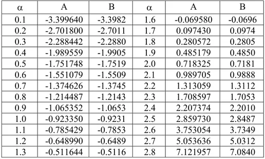
Results of both our calculations and those of Hocking and Rivers are given in Table 1. There is good agreement for lower values of , but larger differences appear when approaches
. For instance, compared to ours for 2.9 and 3.0, their values of Q differ from i ours by ~ 2% and ~ 8%. The results also disagree to a lesser extent for smaller . For instance, when 0.5, we find Qi -1.751748, compared with Qi -1.7519 from Hocking and Rivers. In any case, it is clear that the tabulated results of Hocking and Rivers should not be relied on to give the precision suggested by their table.
Fig. 1 shows Qi
as a function of . It is apparent that, as we found analytically in section 3, Qi
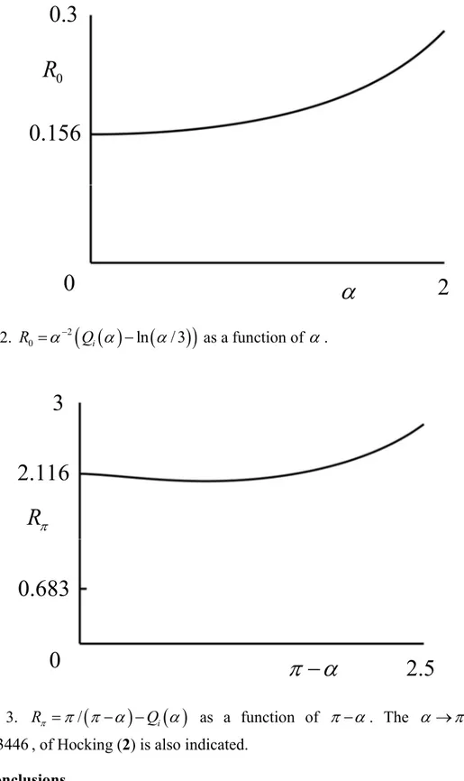
goes from to as increases from 0 to , passing through zero when 0, where 0 1.642671. The leading-order limiting forms, (3.5) as and 0 (3.12) as , are well respected by the numerical results. Because the next-order terms are, by definition, small compared with the leading-order ones, accuracy of their numerical determination is a challenge. Nonetheless, thanks to the intrinsic precision of the present scheme, clear results emerge. Fig. 2 plots the difference between Qi
and the logarithmic form, (3.5), divided by . It appears that the next term in the small-2 expansion (3.5) is
2O , the numerically determined coefficient of that term being 0.156 .
A B A B 0.1 -3.399640 -3.3982 1.6 -0.069580 -0.0696 0.2 -2.701800 -2.7011 1.7 0.097430 0.0974 0.3 -2.288442 -2.2880 1.8 0.280572 0.2805 0.4 -1.989559 -1.9905 1.9 0.485179 0.4850 0.5 -1.751748 -1.7519 2.0 0.718325 0.7181 0.6 -1.551079 -1.5509 2.1 0.989705 0.9888 0.7 -1.374626 -1.3745 2.2 1.313059 1.3112 0.8 -1.214487 -1.2143 2.3 1.708597 1.7053 0.9 -1.065352 -1.0653 2.4 2.207374 2.2010 1.0 -0.923350 -0.9231 2.5 2.859730 2.8487 1.1 -0.785429 -0.7853 2.6 3.753054 3.7349 1.2 -0.648990 -0.6489 2.7 5.053636 5.0312 1.3 -0.511644 -0.5116 2.8 7.121957 7.0840
1.4 -0.371022 -0.3710 2.9 10.914176 10.6700 1.5 -0.224612 -0.2246 3.0 20.084725 21.6400
TABLE 1. Values of Qi
according to the present calculations (A) and Hocking and Rivers (B).FIG. 1. Numerically determined Qi
.Concerning the limit , Fig. 3 shows the difference between Qi
and the limiting form, (3.12), implying~
i
Q C
(5.1)
as . The first term in (5.1) corresponds to (3.12), whereas the second is a higher-order correction. Our numerical results indicate C 2.116, which is clearly different from the value, C2ln 2
0.683446, obtained from [I.3.29]. Given the opacity of the analysis leading to that equation, it is difficult to know the precise reasons for this higher-order discrepancy. However, it seems to us that even the first step in the analysis, namely the approximation of the integral equation by [I.3.21], although justified at leading order, is inadequate at the order considered here. Our numerical results suggest a value close toln 2 2 2.115932
C and, although being unable to prove it, we conjecture that this is the exact value.
0
20
0
5
FIG. 2. 2
0 i ln / 3
R Q as a function of .
FIG. 3. R /
Qi
as a function of . The limiting value, 0.683446 , of Hocking (2) is also indicated.6. Conclusions
The function Qi
, defined by Hocking and Rivers (1), plays a key role in the asymptotic theory of liquid/gas flows with moving contact lines on a wall. In this paper, we have described a new numerical method for its calculation, which we believe to be more accurate than its predecessors because, in dealing with the underlying integral equation, it takes3
0.3
2.116
R
0.683
0
2.5
0R
0.156
0
2
explicit account of a logarithmic singularity and uses a higher-order scheme for the nonsingular part of the integrand. We have given results obtained using this method and compared them with those of Hocking and Rivers (1). The agreement is good at smaller values of , though not perfect, and less so as is approached. The limits and 0
have also been examined. Our results agree with Hocking (2) at leading order, i.e.
~ ln
/ 3
i
Q as and 0 Qi
~ /
as . However, Hocking did not go beyond leading order for and we believe his result for the next order as 0 to be incorrect. Our results indicate that the next order term in the small expansion is O
, 2the numerically determined coefficient of that term being 0.156, while as , the expansion proceeds as Qi
~ /
, where C C 2.116, whereas Hocking claimed that C2ln 2
0.683446, where is Euler’s constant. Our numerical value of C is close to ln 2 2 2.115932 and, although being unable to prove it, we conjecture that this is the exact value.We hope that the numerical scheme and results presented here will interest those, be they theorists or those inclined to numerical simulation, wanting to exploit matched asymptotic methods for the study of flows with moving contact lines.
Acknowledgement
This work was carried out with support from the French ANR research agency, project number ANR-15-CE08-0031, also known as ICEWET.
Appendix A: Demonstration of equation (3.6) Let
/ 1 1 ˆ 4 n n e e L n e n n
(A.1)for 0. Differentiating (A.1),
/ 2 1 / 2 1 ˆ 1 4 1 sinh 2 n n n n dL e e n e d n e
. (A.2) We have
/ / / 1 0 / 2 / 1 1 1 2 cosh 1 n n n n d d n e e d d e e e
. (A.3)Combining (A.2) and (A.3), 2 ˆ sinh 4 cosh 1 dL d . (A.4)
According to (A.1), Lˆ
as 0 , hence the integral of (A.4) gives ˆL
L
for 0 , where (2.2) has been used. Thus, (3.6) applies when 0. Because both the left- and right-hand sides of that equation are even functions of , it also holds for 0.
Appendix B: Calculation of K0
, K1
and K2
0
K , K1
and K2
are given by (2.8), (4.8) and (4.9). The fact that L
is an even function implies
0 2 0 0 0 K K K , (B.1)
1 1 K K . (B.2)
2 2 2 0 2 K K K . (B.3)Thus, we can restrict attention to 0. The values of K0
, K1
and K2
are then required at n , 0 n 4N.Using (3.6) to determine L
, K0
, K1
and K2
gives series which are rapidly convergent when is large and positive. They are numerically calculated by truncation:
/ 1 1 4 K n n e e L n e n n
, (B.4)
/ 0 2 2 1 1 4 K n n e e K n e n n
, (B.5)
1 2 1 / 2 1 4 K n n e K n n e n e n n
, (B.6)
2 2 2 2 1 2 2 / 2 1 2 2 4 2 2 K n n e K n n n e n e n n n
. (B.7)(B.4)-(B.7) provide L
, K0
, K1
and K2
for 4N. However, convergence is slower when is reduced and a different method is needed.According to (2.2), (2.8), (4.8) and (4.9), 2 ˆ 1 sinh 2 4 cosh 1 dL d , (B.8) 0 ˆ 1 ˆ 2 dK L d , (B.9) 1 ˆ 1 ˆ 4 dK L d , (B.10) 2 2 ˆ 1 ˆ 6 dK L d , (B.11) where 1 ˆ ln 2 L L , (B.12) 0 0 1 ˆ ln 2 K K , (B.13) 2 1 1 1 ˆ ln 4 K K , (B.14) 3 2 2 1 ˆ ln 6 K K . (B.15)
The change of variables from L , K , 0 K and 1 K to 2 ˆL, K , ˆ0 Kˆ1 and Kˆ2 removes the singularity at 0. A fourth-order Runge-Kutta scheme with step is used to integrate (B.8)-(B.11) downwards in , beginning at 4N and values of ˆL, K , ˆ0 Kˆ1 and Kˆ2 from (B.12)-(B.15), with those of L , K , 0 K and 1 K from (B.4)-(B.7). The step length is 2
/ M
obtained using (B.13)-(B.15) every M steps. To maintain precision at small , M is chosen to be the smallest integer greater than 1.
References
1. L. M. HOCKING and A. D. RIVERS, ‘The spreading of a drop by capillary action’, J. Fluid Mech. 121 (1982) 425-442.
2. L. M. HOCKING, ‘A moving fluid interface. Part 2. The removal of the force singularity by a slip flow’, J. Fluid Mech. 79 (1977) 209-229.
3. H. K. MOFFATT, ‘Viscous and resistive eddies near a sharp corner’, J. Fluid Mech. 18 (1964) 1-18.
4. C. HUH and L. E. SCRIVEN, ‘Hydrodynamic model of steady movement of a solid/liquid/fluid contact line’, J. Colloid. Interf. Sci. 35 (1971) 85-101.
5. D. BONN, J. EGGERS, J. INDEKEU, J. MEUNIER and E. ROLLEY, ‘Wetting and spreading’, Rev. Mod. Phys. 81 (2009) 739-805.
6. L. M. HOCKING, ‘Sliding and spreading of thin drops’, Q. J. Mech. Appl. Math. 34 (1981) 37-55.
7. R. G. COX, ‘The dynamics of the spreading of liquids on a solid surface. Part 1. Viscous flow’, J. Fluid Mech. 168 (1986) 169-194.
8. Y. SUI and P. D. M. SPELT, ‘Validation and modification of asymptotic analysis of slow and rapid droplet spreading by numerical simulation’, J. Fluid Mech. 715 (2013) 283-313. 9. Y. SUI, H. DING and P. D. M. SPELT, ‘Numerical simulations of flows with moving contact lines’, Annu. Rev. Fluid Mech. 46 (2014) 97-119.
10. Y. SUI and P. D. M. SPELT, ‘An efficient computational model for macroscale simulations of moving contact lines’, J. Comput. Phys. 242 (2013) 37-52.
11. Z. SOLOMENKO, P. D M. SPELT and P. ALIX, ‘A level-set method for large-scale simulations of three-dimensional flows with moving contact lines’, J. Comput. Phys. 348 (2017) 151-170.