HAL Id: hal-02405950
https://hal.umontpellier.fr/hal-02405950
Submitted on 17 Nov 2020
HAL is a multi-disciplinary open access
archive for the deposit and dissemination of
sci-entific research documents, whether they are
pub-lished or not. The documents may come from
teaching and research institutions in France or
abroad, or from public or private research centers.
L’archive ouverte pluridisciplinaire HAL, est
destinée au dépôt et à la diffusion de documents
scientifiques de niveau recherche, publiés ou non,
émanant des établissements d’enseignement et de
recherche français ou étrangers, des laboratoires
publics ou privés.
Unveiling dimensions of stability in complex ecological
networks
Virginia Domínguez-García, Vasilis Dakos, Sonia Kéfi
To cite this version:
Virginia Domínguez-García, Vasilis Dakos, Sonia Kéfi. Unveiling dimensions of stability in complex
ecological networks. Proceedings of the National Academy of Sciences of the United States of America
, National Academy of Sciences, 2019, pp.201904470. �10.1073/pnas.1904470116�. �hal-02405950�
DRAFT
Unveiling dimensions of stability in complex
ecological networks
Virginia Dominguez-Garcìaa,1, Vasilis Dakosa, and Sonia Kéfia aISEM, CNRS, Univ. Montpellier, IRD, EPHE, Montpellier, France.
This manuscript was compiled on November 28, 2019
Understanding the stability of ecological communities is a matter of increasing importance in the context of global environmental change. Yet, it has proved to be a challenging task. Different metrics are used to assess the stability of ecological systems, and the choice of one metric over another may result in conflicting conclusions. Although each of the multitude of metrics is useful for answering a specific question about stability, the relationship among metrics is poorly un-derstood. Such lack of understanding prevents scientists from devel-oping a unified concept of stability. Instead, by investigating these relationships we can unveil how many ‘dimensions’ of stability there are (i.e. in how many independent components stability metrics can be grouped), which should help building a more comprehensive con-cept of stability. Here, we simultaneously measured 27 stability met-rics frequently used in ecological studies. Our approach is based on dynamical simulations of multispecies trophic communities under different perturbation scenarios. Mapping the relationships between the metrics revealed that they can be lumped into three main groups of relatively independent stability components: ‘early response to pulse’, ‘sensitivities to press’ and ‘distance to threshold’. Selecting metrics from each of these groups allows a more accurate and prehensive quantification of the overall stability of ecological com-munities. These results contribute to improving our understanding and assessment of stability in ecological communities.
stability | food webs | networks | ecological community
S
tability has been a core topic of research in complex sys-tems across disciplines. From socioeconomic models of political regimes (1,2), to financial systems (3–5), social or-ganizations (6,7) or biological systems of genetic regulatory circuits (8,9), the study of dynamical stability keeps drawing the attention of the scientific community. This interest has been particularly prominent in ecology, where it has fuelled decades of research (10–15). Yet, progress in understanding what determines the stability of complex systems such as ecological communities has been hampered by unclear, and sometimes, conflicting results. One of the main reasons has proved to be the broad definition of the concept of stability itself (12), which has led to confusion and a lack of clear guidelines about the practical quantification of stability in empirical studies (14,16). Probably one of the best examples of this confusion is the long standing controversy of how sta-bility varies with species diversity (17). While some studies have shown that biodiversity can enhance stability (18–20), others have found the opposite result (21–23), both effects (24), or even non-monotonous relationships (25). The expla-nation behind this apparent contradiction is that stability is a multidimensional concept: it has several ‘facets’ and can be described by different metrics, which do not all vary positively with biodiversity (13, 24,26). While the multidimensional nature of the stability concept has been well recognized inthe literature (10–12), our understanding of it has remained limited (14). The vast majority of studies typically include only one metric of stability at a time, and the few studies that have simultaneously measured multiple metrics of stability have considered them as independent when, in fact, it has been acknowledged that they could be interdependent (27). This possible interdependence implies that measuring multiple metrics may more broadly estimate stability to the extent that these metrics quantify relatively independent components of stability. Therefore, to advance towards a thorough and more systematic assessment of ecological stability, we need to understand how stability can be decomposed into different components – also referred to as ‘dimensions’ in the literature (27) – and if so, how many there are and how they can be best
measured.
We tackle this challenge from a theoretical perspective by investigating the interdependence of stability metrics in trophic ecological networks. Combining structural food-web models (28) with bioenergetic consumer-resource models (29,30), we simulate the dynamics of multispecies trophic communities un-der different perturbation scenarios. Perturbations are changes in the biotic or abiotic environment that alter the structure and dynamics of communities (14,31). We consider three main types of perturbations: pulse (32), i.e. instantaneous dis-turbances, after which community recovery can be measured (e.g. forest fires or floods), press (32), i.e. lasting disturbances after which post-perturbed communities can be compared to pre-perturbed ones (e.g. climatic changes or extinction of a species), and environmental stochasticity (33–35), where com-munities are constantly affected by small external changes. We quantify the stability of our simulated communities to these perturbations with 27 metrics frequently used in the ecological literature (see Table1). We then explore how these
Significance Statement
While the need to consider the multidimensionality of stability has been clearly stated in the ecological literature for decades, little is known about how different metrics of stability relate to each other in ecological communities. By simulating mul-tispecies trophic networks, we measure how frequently-used stability metrics relate to each other, and we identify the inde-pendent components they form based on their correlations. Our results open a way to a simplification and better understanding of the overall stability of ecological systems.
S.K., V.D.-G. and V.D. designed the study. V.D.-G. performed the simulations and their analysis. S.K., V.D.-G. and V.D. discussed the results. All authors contributed to the writing of the manuscript. The authors declare no conflict of interest.
1To whom correspondence should be addressed. E-mail:[email protected]
DRAFT
metrics correlate with each other. If metrics are found to beuncorrelated, that would mean that they all inform very dif-ferent aspects of stability of an ecological community and that a more coherent concept of stability currently lacks empirical support. In the opposite case, if all metrics are found to be perfectly correlated with each other, considering only a single metric would be enough to assess the overall stability of an ecological community. Therefore, by studying the correlations between stability metrics, we can evaluate whether the dif-ferent metrics considered provide similar information about the stability of an ecological community or whether they form distinct groups that reflect partly independent ‘dimensions’ of community stability.
Results and Discussion
Community size and stability metrics’ correlations.
Commu-73
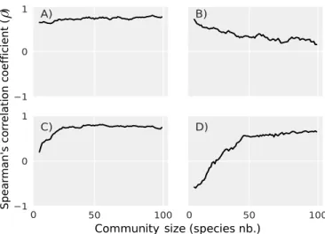
nity size (i.e. the number of species) has been shown to play a fundamental role in the stability of ecological networks, al-though it is not entirely clear if it promotes their stability, hinders it, (13) or both (24,25). For example, a food web simulation study showed that persistence (i.e. the fraction of surviving species) and population variability were either negatively or positively correlated depending on the species richness of the community (25). We therefore start by investi-gating if the pairwise correlations between the stability metrics are affected by community size in our simulated trophic com-munities. Overall, many pairwise correlations (~44% out of the 351 correlation pairs) are not highly affected by commu-nity size (Fig1A). Some pairwise correlations (~32%) become weaker as community size grows (Fig.1B), while others (~20%) become stronger (Fig.1C). In a few cases (~3%), the correla-tion between two metrics can switch sign as community size changes (Fig.1D). The dependence of pairwise correlations on community size is especially present in communities with less than 50 species. In contrast, most correlations (~94%) remain largely constant in species-rich communities (> 50 species; SI Appendix Fig. S1). Given the dependence of pairwise correlations on community size, we next study stability metric correlations across three levels of species richness: small (5 to 15 species), medium-sized (45 to 55 species), and large communities (85 to 95 species). In what follows, we present the results for medium-sized communities, while the results for small and large communities can be found in the SI Appendix. Three groups of stability metrics.To explore if there is any
101
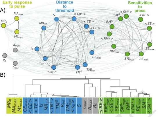
structure in the way metrics are correlated with each other, we build a network of stability metrics in which nodes repre-sent the metrics and links their weighted (unsigned) pairwise correlations (see Materials and Methods). Using a community detection algorithm based on maximizing modularity (see Ma-terials and Methods), we find that metrics form three distinct groups such that metrics that belong to the same group are more strongly correlated with each other than with metrics outside of their group (Fig.2A and SI Appendix Fig. S3).
The ‘early response to pulse’ group (light green in Fig. 2A) contains measures of the initial and short-term deviations of a community from its reference state after a pulse perturbation. The ‘sensitivities to press’ group (green in Fig. 2A) includes metrics that quantify changes in total and individual species’ biomass between post- and pre-perturbed communities after a press perturbation. The ‘distance to threshold’ group (blue in
1 0 1 50 100 1 0 1 50 100 A) B) C) D) 0 0
Community ize (species nb.)s
Spea rman's co rr elati on c oeffic ient ( )
Fig. 1. https://www.overleaf.com/project/5c361f3e4b0f20641e21ee84 Spearman’sρ
pairwise correlation coefficient between stability metrics as a function of community size (i.e. number of species at steady state). A) Some pairwise correlations are not affected by community size, e.g. correlation between two metrics of tolerance to increased mortality at a global (i.e. community) and local (i.e. species) scale (resp.T MGand< T ML>). B) Some metrics are only strongly correlated in small communities, e.g. correlation between ‘stochastic invariability’ (Is) and ‘time to maximum amplification’ (tmax). C) Other metrics are only strongly correlated in large communities, e.g. correlation between resilience’ (Rinf) and the average strength of the sensitivity matrix (< sij>). D) Some pairwise correlations change sign with community size, e.g. correlation between the resistance of total biomass (RMG) and the sensitivity of species biomass to a global increase in mortality (SMG). See Table1and Materials and Methods for metrics definitions.
Fig. 2A) consists of metrics that measure how easily a system crosses thresholds to new dynamical states, for example the amount of external pressure before a community experiences an abrupt change, the closeness of the rarest species to extinction, the population variability, and secondary extinctions caused by random extinctions.
Three metrics (in gray in Fig. 2A) were not clearly assigned to any of the three groups (see SI, section 2). These metrics include measures of the initial and transient responses of the most abundant species to pulse perturbations. Because of their idiosyncratic correlations with the rest of the metrics, we kept them apart from the other metrics.
Interestingly, the three emergent groups split metrics in terms of both the temporal scale of the response and the type of perturbation. Indeed, the ‘early response to pulse’ group only contains metrics describing transient behavior, while the ‘sensitivities to press’ and ‘distance to threshold’ groups contain metrics describing long-term (asymptotic) dynamics. Furthermore, the ‘early response to pulse’ and ‘sensitivities to press’ form two contrasting groups containing metrics that respectively refer to pulse and press perturbations, while met-rics in the ‘distance to threshold’ group refer to both types of perturbations. The weak correlations between the three groups of metrics (with an average correlation of ~0.13 ; SI Appendix Fig. S2 and section 3) suggests that the metrics within a group can be considered as relatively independent from metrics in other groups. Therefore, these three groups reflect major components that constitute different dimensions of the stability of trophic communities (27) that should be mea-sured in an ecological community to comprehensively assess its overall stability.
Further studying the degree of (dis)similarity between the
DRAFT
A)
MR
0MA
maxMt
maxCE
max<
CE
>
<
TE
>
Is
MR
inf < TM L>TM
GR
infTM
L min<
s
ij>
S t
maxA
maxR
0<
RE
>
RM
L max<
SE
>
SE
maxSM
L maxRM
G < RM L>RE
maxSM
G < SM L> MR0 MAmax Mtmax CEmax < TE > Is MRinf < TML> TMG Rinf TML min < sij> S tmax Amax R0 < RE > RML max < SE > SEmax SML max RMG < RML> REmax SMG< SM L> < CE >B)
Early response to pulse Sensitivities to press Distance to thresholdFig. 2. A) Network of stability metrics for
medium-sized communities (45 to 55 species). Nodes represent stability metrics and the thick-ness of links their unsigned pairwise Spear-man’sρcorrelation coefficients. Node col-ors distinguish the three groups identified by the modularity algorithm, with a modularity of
Q=0.177: ‘early response to pulse’ group in light green, ‘distance to threshold’ group in blue, and ‘sensitivities to press’ group in darker green. In grey are metrics that the modular-ity algorithm was not able to unambiguously place in any group. B) Hierarchical cluster-ing applied to the network of stability metrics. Correlations are used to compute a distance between all pairs of metrics, which are repre-sented here by a dendrogram. The key to inter-preting such a dendrogram is to focus on the first ‘branch’ at which any two metrics are joined together; the further away two metrics are from this ‘common ancestor’, the less similar they are. The goodness-of-fit of distances based on the dendrogram to the distances in the original data (pairwise correlations) is quantified by the Cophenetic Coefficient (c =0.85). Metrics are clustered similarly as by the modularity parti-tioning, except for the ‘resistance to extinction’ metric, (< RE >) represented with a stripped pattern, which is therefore considered to not clearly belong to one of the groups in upcoming analyses. See Table 1 for metrics’ definitions.
different stability metrics with a hierarchical clustering analysis (36,37) (see Materials and Methods) confirms the partitioning found by the modularity algorithm, except for one outlier metric (striped in Fig. 2B), which was not attributed to the same group by both analyses (see SI, section 4) and is therefore not considered to clearly belong to one of the three groups for subsequent analyses. The generated dendogram allows to visualize a more detailed structure, with subgroups of highly similar metrics within the three groups identified by the modularity algorithm (See SI, section 4). Practically, this implies that for these sets of highly similar metrics, only one of the metrics could be selected interchangeably. Moreover, some of these close similarities could also be of theoretical interest. For example, in the ‘Distance to threshold’ group, we find five strongly connected metrics of very different nature: resilience (a metric of dynamical stability,Rinf), tolerance metrics (which assess structural stability; T MG, T MminL ), and sensitivity metrics (which are based on the inverse Jacobian; S, < sij>). Some of these connections have been previously reported (38,39), but we still lack a complete theoretical map of most metrics’ relationships.
The sign of the correlations between stability metrics.The
171
sign of the correlations between metrics is important because negative correlations between metrics would suggest trade-offs: promoting stability according to one of the metric would happen at the expense of stability according to another metric. In our simulated trophic communities, however, we only find a few negative correlations (see SI Appendix section 5 and Fig. S4). Most of the negative correlations are identified in small communities (below 20 species) between metrics of ‘resistance’ (i.e. total change in aggregated community biomass before
and after a press perturbation) and ‘sensitivity’ (total change in species’ populations after a press perturbation; Table1). In fact, in communities of more than 20 species, there is only
one relatively strong negative correlation (ρ ∼ −0.4) between ‘reactivity’ (R0) and ‘time to maximum amplification’ (tmax). The relationship between these two metrics has been previously studied and found to be complex (40). Our results here suggest that communities whose abundant species initially deviate fast from their original state (i.e. high R0), are also those that
tend to start recovering early (i.e. low tmax); conversely, communities with abundant species that are less reactive tend to take longer before they start their recovery.
The vast majority of positive correlations (from ~86% of all 351 pairs in small communities to ~93% in large communities) found here is in line with recent experimental findings, where multiple positive correlations between stability metrics were found in communities of similar size as our simulated com-munities (24,27). For example, we find a positive correlation (ρ =0.54) between invariability (Is) and resistance to small press perturbations (S) in agreement with (24). We also find a positive correlation (ρ =0.57) between invariability (Is) and the number of secondary extinctions (< CE >), in communi-ties of similar sizes as those studied by (27). In light of this, stability trade-offs seem to be a rare exception in complex trophic communities.
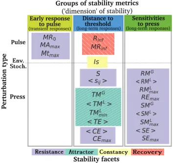
Mapping the stability metrics.Past reviews of stability in ecol-ogy have highlighted the multidimensional nature of stability and have attempted at grouping metrics in a few stability ‘facets’ based on the similarity in their definition (10–13). Here, three relatively independent groups of metrics emerged from the analysis of the correlations between metrics, and we argue that these groups can be interpreted as different ‘dimensions’ of stability. In what follows, we map all metrics according to their stability group (or ‘dimension’), perturbation type, and stability facet in an attempt to better understand the relationships between these different categories (Fig. 3).
DRAFT
Resistance Attractor Constancy Recovery Stability facets
Early response
to pulse Sensitivitiesto press Pulse Press Env. Stoch. Pertur bat ion type
Groups of stability metrics
('dimension' of stability)
Distance to threshold
(transient responses) (long-term responses) (long-term responses) MR0 MAmax Mtmax CEmax < CE > Is MRinf Rinf < TE > < TML> TMG TML min < sij> S REmax RML max SEmax SML max < SE > RMG < RML> SMG < SML>
Fig. 3. Classification of the stability metrics according to three axes: the perturbation
type (pulse, press or environmental stochasticity), the stability group (‘early response to pulse’, ‘distance to threshold’, and ‘sensitivities to press’) and the stability facets typically describing stability properties in the literature. There is currently no consen-sus on the names of these facets; we here refer to them as ‘resistance’ in purple (how much the system changes under a press perturbation), ‘attractor’ in green (the type and number of attractors of the system), ‘constancy’ in yellow (how variable the system is), and ‘recovery’ in red (if and how the system recovers from a pulse perturbation) (15). Colors of the groups of stability metrics are the same as in Fig.2. Metrics not clearly associated to one of the three groups in Fig.2(i.e. the metrics in grey and< RE >) were not included here. See Table 1 for metrics’ definitions.
stability groups don’t map one-to-one. For example, resistance metrics can belong to all three stability groups, while metrics from the four stability facets can be highly correlated with each other and belong to the same stability group (e.g. the ‘distance to threshold’ group). More strikingly, our mapping shows that it is not possible to simultaneously capture the three stability ‘dimensions’ with an experiment that would involve only one type of perturbation. Early response to pulse, i.e. transient responses (Fig. 3 left), can only be studied in communities that experience a pulse perturbation, while all ‘resistance’ and ‘sensitivity’ of biomass metrics are, by definition, the results of a press perturbation. The fact that knowledge about stability to a given type of perturbation does not extend to another type of perturbation confirms that we cannot get away from specifying the stability ‘of what’ and ‘to what’ (14,16).
Conclusion.Perhaps the most important finding of our
analy-234
sis is that the multiplicity of stability metrics can essentially be mapped into three relatively independent groups that reflect three different components, or ‘dimensions’, of stability. This suggests that the dimensionality of the stability of trophic ecological communities is much lower than the number of met-rics used to quantify it, and that stability could therefore be assessed using a small number of metrics.
Each of the many stability metrics allows addressing spe-cific questions by quantifying a given aspect of stability. At the same time, however, the grouping of many metrics in just a few components raises the question of which specific metrics
to choose if one wants to assess the overall stability of an eco-logical system. An intuitive guess is that combining metrics from each of the three groups could be a way of decreasing the amount of metrics used, while still accurately estimating the multiple ‘dimensions’ of the stability of an ecological com-munity. Preliminary analyses suggest that using only three metrics – those with the highest explained variance in each of the groups – explains respectively 54%, 52% and 59% of the original variance in small, medium and large communities (see SI, section 6 for more details). Moreover, analyses of the vol-ume of the covariance ellipsoid confirm that selecting metrics from the three different groups , rather than the same number of metrics from the same group, best describes the different stability ‘dimensions’ (see SI, section 7 and Fig. S7). However, due to the high correlations between metrics within a group, it is difficult to propose a single best way of selecting metric(s) in each of the groups. Although the choice of the metrics will always depend on the system studied and on practical constraints, hierarchical analyses (Fig. 2B and SI Appendix Fig. S3) and explained variance analyses (SI Appendix section 6) can help making informed choices.
Interestingly, our analysis confirms previously known re-lationships between metrics, but it also reveals unexpected dependencies, which could either be due to mathematical rela-tionships yet to be investigated or because the metrics actually expose latent dimensions of stability. Although, our approach does not elucidate the causes for the metrics’ correlations, it does point towards future areas of research. In that sense, our results are of interest to both theoreticians – because they hint towards yet unknown mechanisms underlying correlations between stability metrics –, as well as to experimentalists, who can use the patterns of correlations to choose which metrics to evaluate in their experiments.
Finally, although our study focuses on the stability of food webs, the relationships found here could be of interest to understand the stability of other types of networks, in ecology as well as in other disciplines. In fact, even if the exact number of identified groups of metrics could be altered in other systems or by the incorporation of additional stability metrics, the framework we propose is flexible enough to accommodate to different conditions and opens a way towards simplifying the study of overall stability in different types of complex dynamical system. After all, directed networks of many kinds describe transport of matter, information, or capital in a similar way as food webs describe fluxes of biomass from primary producers to apex predators.
Materials and Methods
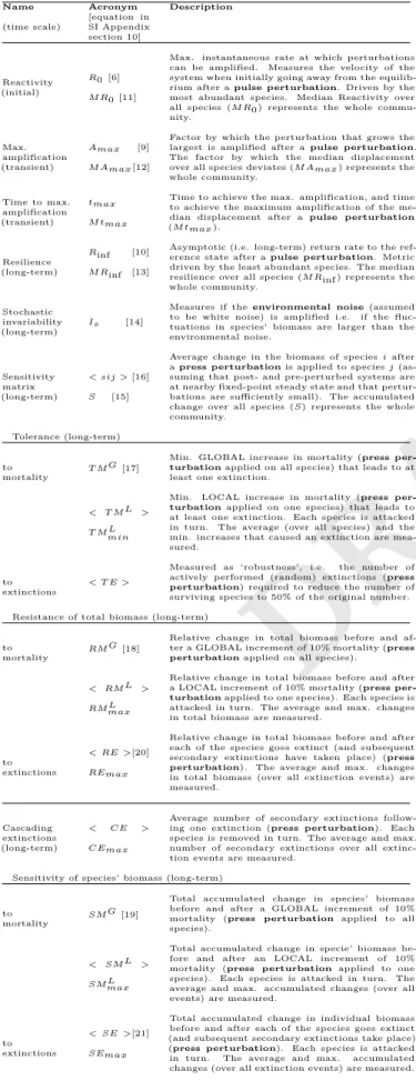
Stability metrics. We review the ecological literature to identify the most frequently used metrics for assessing community stability. Specifically, we consider metrics that quantify stability in commu-nities that yield stable (fixed equilibrium) dynamics. We do not consider measures of community invasibility. For metrics that can be quantified in multiple ways, we only retain a single way of mea-suring that metric. With these criteria, we obtain 27 metrics that are described in Table1, specifying their temporal scale (below the name) and the type of perturbation they are associated to (in bold letters in the description). Metrics include analytical responses to small pulse perturbations - i.e. instantaneous disturbances causing a sudden change in species abundances - obtained from the com-munity matrix (or Jacobian) covering initial (reactivity), transient
DRAFT
Table 1. Stability metrics’ names, characteristic time scales, defi-nitions, and, when relevant, reference to the equation in the SI Ap-pendix, section 10 (See Material and Methods for a guide to the met-rics acronyms)
Name Acronym Description (time scale) [equation in SI Appendix section 10] Reactivity (initial) R0 [6]... ... M R0 [11]
Max. instantaneous rate at which perturbations can be amplified. Measures the velocity of the system when initially going away from the equilib-rium after a pulse perturbation. Driven by the most abundant species. Median Reactivity over all species (M R0) represents the whole commu-nity. Max. .... amplification (transient) Amax [9] ... ... M Amax[12]
Factor by which the perturbation that grows the largest is amplified after a pulse perturbation. The factor by which the median displacement over all species deviates (M Amax) represents the whole community. Time to max. amplification (transient) tmax ... ... M tmax
Time to achieve the max. amplification, and time to achieve the maximum amplification of the me-dian displacement after a pulse perturbation (M tmax). Resilience (long-term) Rinf [10] ... ... M Rinf [13] ..
Asymptotic (i.e. long-term) return rate to the ref-erence state after a pulse perturbation. Metric driven by the least abundant species. The median resilience over all species (M Rinf ) represents the whole community.
Stochastic invariability (long-term)
Is...[14]
Measures if the environmental noise (assumed to be white noise) is amplified i.e. if the fluc-tuations in species’ biomass are larger than the environmental noise. Sensitivity matrix .. (long-term) < sij > [16] .. ... S..[15]
Average change in the biomass of species i after a press perturbation is applied to species j (as-suming that post- and pre-perturbed systems are at nearby fixed-point steady state and that pertur-bations are sufficiently small). The accumulated change over all species (S) represents the whole community.
Tolerance (long-term)
to mortality
T M G [17]
Min. GLOBAL increase in mortality (press per-turbation applied on all species) that leads to at least one extinction.
< T M L >
...
T M L min
Min. LOCAL increase in mortality (press per-turbation applied on one species) that leads to at least one extinction. Each species is attacked in turn. The average (over all species) and the min. increases that caused an extinction are mea-sured.
to extinctions
< T E >
Measured as ‘robustness’, i.e. the number of actively performed (random) extinctions (press perturbation) required to reduce the number of surviving species to 50% of the original number. Resistance of total biomass (long-term)
to mortality
RM G [18]
Relative change in total biomass before and af-ter a GLOBAL increment of 10% mortality (press perturbation applied on all species).
< RM L >
...
RM Lmax
Relative change in total biomass before and after a LOCAL increment of 10% mortality (press per-turbation applied to one species). Each species is attacked in turn. The average and max. changes in total biomass are measured.
to extinctions
< RE >[20]
...
REmax
Relative change in total biomass before and after each of the species goes extinct (and subsequent secondary extinctions have taken place) (press perturbation). The average and max. changes in total biomass (over all extinction events) are measured. Cascading extinctions (long-term) < CE > ... ... CEmax
Average number of secondary extinctions follow-ing one extinction (press perturbation). Each species is removed in turn. The average and max. number of secondary extinctions over all extinc-tion events are measured.
Sensitivity of species’ biomass (long-term)
to mortality
SM G [19]
Total accumulated change in species’ biomass before and after a GLOBAL increment of 10% mortality (press perturbation applied to all species).
< SM L >
.. ...
SM Lmax
Total accumulated change in specie’ biomass be-fore and after an LOCAL increment of 10% mortality (press perturbation applied to one species). Each species is attacked in turn. The average and max. accumulated changes (over all events) are measured.
to extinctions
< SE >[21]
...
SEmax
Total accumulated change in individual biomass before and after each of the species goes extinct (and subsequent secondary extinctions take place) (press perturbation). Each species is attacked in turn. The average and max. accumulated changes (over all extinction events) are measured.
(maximum amplification and time to maximum amplification), and asymptotic (resilience) temporal regimes, both quantified at the individual species level and at the community level (21,40,41). Responses to environmental noise is assessed with the stochastic invariability metric (34). Analytical responses to small press per-turbations - i.e. lasting disturbances causing the abundance of species to be permanently changed - are measured by means of the sensitivity matrix (inverse of the Jacobian matrix) (32,38,42). We also apply two different types of more intense press perturbations empirically: an increase in mortality both at the local (i.e. only on one individual species at a time) and at the global (i.e. on 318 all species of the community simultaneously) scales, and random 319 extinctions of species. Structural stability (43,44) to these two 320 types of press perturbations is assessed with the tolerance metrics 321 (Table1). Tolerance to mortality is measured as in previous studies 322 (45,46), and tolerance to extinctions is measured with robustness 323 (47). We also include metrics of community resistance to random 324 extinctions (48) as cascading extinctions. Empirical measures of 325 resistance to both types of press perturbations, named resistance of 326 total biomass and sensitivity of species’ biomass, are also quantified 327 in a similar fashion as in previous studies (49). All the metrics 328 are defined in such a way that an increase in their value means an 329 increase in community stability. Definitions of metrics can be found 330 in SI, section 10, and the dataset of stability metrics in SI Dataset 331
S1. 332
The acronyms of the metrics that quantify responses to empirical 333 press perturbations are encoded as follows: the first letter represents 334 if they are a measure of tolerance (T) resistance (R), or sensitiv-ity (S), followed by the initial letter of the perturbation, which is either mortality (M) or random extinctions (E). The superscript differentiates, when needed, if the perturbation is global (G) (i.e applied on all species of the communities as the same time) or local (L) (i.e. applied on one species at a time). When nothing is indi- cated, the perturbation is assumed to be local. In the case of local perturbations, the subscripts min and max indicate whether the metric is the extreme (resp. minimum or maximum) value observed, while the brackets <> indicate that the metric is the average of all observed values.
Generating communities and model simulations. We use the niche model (28) to construct food-web communities. We then use the produced community structure to simulate the biomass of each species using a bioenergetic consumer-resource model with allometric constraints (30): dBi dt = riGiBi+Bi X j∈prey e0jFij− X k∈pred BkFki−xiBi−diBi [1]
where the interaction term Fijis defined as:
Fij=
wiaijB1+qj
mi(1 + wiPk∈preyaikhikB1+qk )
[2] 353 During the simulations, species biomass adjust dynamically and some extinctions may occur before a steady state is achieved. Thus, the species that comprise the final dynamical trophic networks are selected by structural constraints and energetic processes among the species. We fix the parameter of the functional response to q = 0.3 and the predator/prey body-mass ratio to Z = 1.5. Values for all the other scaling parameters are averages of values presented in (50). We generate networks with an initial species richness ranging from 5 to 115 species and a fixed connectance of c = 0.15. During the simulations, if species biomass crossed the extinction threshold (1E−6m
i), we consider that species extinct. If more than 10% of the
initial number of species goes extinct, we discard this community. Following this procedure, we simulate more than 10000 different dynamical trophic communities with species richness ranging from 5 to 105 species. For more details, see SI, sections 8 and 9. Pairwise correlations and networks of stability metrics. For each com-munity size, ranging from 5 to 100 species (with a step of 1), we sample 100 trophic communities of each size (SI Dataset S2) and compute the pairwise correlations among all stability metrics using Spearman’s correlation rank, ρ. We consider that pairwise correla-tions remain unchanged throughout a gradient of species richness if
DRAFT
the variation in the correlation between the initial and final com-375
munity sizes (∆ρ) is below 0.1. We use the pairwise correlations 376
to build a network of stability metrics. In this network, each node 377
is a metric and the links are the pairwise correlations between the 378
metrics. The links are weighted (i.e the stronger the correlation the 379
thicker the link) and unsigned (i.e. we consider absolute correlations 380
and ignore if two metrics are negatively or positively correlated). 381
We assemble in this way networks of stability metrics for different 382
classes of community sizes: small (5-15 species), medium (45-55 383
species), and large (85-95 species) communities by considering the 384
average value of correlations (i.e. average ρ) within these size ranges. 385
Grouping stability metrics. We search for groups of metrics 386
in the stability network such that pairs of metrics are more 387
strongly correlated to other metrics of the same group than to 388
metrics in other groups. Modularity quantifies the quality of a 389
particular partition of a network into such ‘clusters’ (i.e. groups 390
of nodes) (51). The modularity algorithm detects clusters 391
by searching over many possible partitions of a network and 392
finding the one that maximizes modularity (52). We apply such 393
a community detection algorithm on our pairwise-correlation 394
weighted networks using Gephi (53). We repeat the computa-395
tions 10 times for each network, and we select the partition in 396
clusters that renders the highest value of modularity (i.e. Q=0.177). 397
398
Stability metric (dis)similarity. We use hierarchical clustering (36) 399
to aggregate stability metrics according to their similarity (based on 400
correlation). Starting with the closest pair of metrics, subsequent 401
metrics are joined together in a hierarchical fashion from the closest 402
(i.e most similar) to the furthest apart (most different) until all 403
metrics are included. The distance between a pair of metrics is 404
defined as d = (1 − ρ) where ρ is the Spearman’s rank correlation. 405
We constructed the dendrogram with the hierarchical agglomerative 406
clustering (HAC) algorithm in Python (54). We selected the linkage 407
method (‘average’) that rendered distances in the dendrogram closest 408
to the original pairwise correlation (goodness-of-fit based on the 409
cophenetic correlation coefficient c=0.85). The closer c is to 1, the 410
better the correspondence. 411
ACKNOWLEDGMENTS. The initial idea for this project emerged 412
from discussions with Colin Fontaine. The authors are very grateful 413
for stimulating discussions with him. We would also like to thanks 414
Stéphane Robin for advice on the statistical analyses. We thank the 415
two anonymous reviewers and the editor for their very constructive 416
comments, which have considerably improved the manuscript. This 417
work was funded by the ANR project ARSENIC (ANR-14-CE02-418
0012).
1. Gross T, Rudolf L, Levin S, Dieckmann U (2009) Generalized models reveal stabilizing factors in food webs. Science 325:747–50.
2. Wiesner K, et al. (2018) Stability of democracies: a complex systems perspective. European Journal of Physics 40(1):014002.
3. da Cruz JP, Lind PG (2012) The dynamics of financial stability in complex networks. The European Physical Journal B 85(8).
4. Arinaminpathy N, Kapadia S, May RM (2012) Size and complexity in model financial systems. Proceedings of the National Academy of Sciences 109(45):18338–18343.
5. Bardoscia M, Battiston S, Caccioli F, Caldarelli G (2017) Pathways towards instability in finan-cial networks. Nature Communications 8(1).
6. Hickey J, Davidsen J (2019) Self-organization and time-stability of social hierarchies. PLOS ONE 14(1):e0211403.
7. Prayag G, Chowdhury M, Spector S, Orchiston C (2018) Organizational resilience and finan-cial performance. Annals of Tourism Research 73:193–196.
8. Becskei A, Serrano L (2000) Engineering stability in gene networks by autoregulation. Nature 405(6786):590–593.
9. Reznick E, Segre D (year?) On the stability of metrabolic cycles. Journal of Theoretical Biology 266(4):536–549.
10. Orians GH (1975) Diversity, stability and maturity in natural ecosystems, eds. van Dobben WH, Lowe-McConnell RH. (Springer Netherlands, Dordrecht), pp. 139–150.
11. Pimm SL (1984) The complexity and stability of ecosystems. Nature 307:321–326. 12. Grimm V, Wissel C (1997) Babel, or the ecological stability discussions: an inventory and
analysis of terminology and a guide for avoiding confusion. Oecologia 109(3):323–334. 13. Ives AR, Carpenter SR (2007) Stability and diversity of ecosystems. Science 317:58–62. 14. Donohue I, et al. (2016) Navigating the complexity of ecological stability. Ecology Letters
19(9):1172–1185.
15. Kéfi S, et al. (2019) Advancing our understanding of ecological stability. Ecology Letters 22(9):1349–1356.
16. Grimm V, Schmidt E, Wissel C (1992) On the application of stability concepts in ecology. Ecological Modelling 63(1):143 – 161.
17. McCann KS (2000) The diversity–stability debate. Nature 405(6783):228–233. 18. Tilman D (1994) Biodiversity and stability in grasslands. Nature 367:363–365.
19. Cardinale BJ, et al. (2013) Biodiversity simultaneously enhances the production and stability of community biomass, but the effects are independent. Ecology 94(8):1697–1707. 20. Johnson S, Domínguez-García V, Donetti L, Muñoz MA (2014) Trophic coherence determines
food-web stability. Proceedings of the National Academy of Sciences 111(50):17923–17928. 21. Pimm SL, Lawton JH (1978) On feeding on more than one trophic level. Nature
275(5680):542–544.
22. Yodzis P (1981) The stability of real ecosystems. Nature 289:674–676.
23. Valdivia N, Molis M (2009) Observational evidence of a negative biodiversity–stability relation-ship in intertidal epibenthic communities. Aquatic Biology 4:263–271.
24. Pennekamp F, et al. (2018) Biodiversity increases and decreases ecosystem stability. Nature 563:109–112.
25. Brose U, Williams RJ, Martinez ND (2006) Allometric scaling enhances stability in complex food webs. Ecology Letters 9(11):1228–1236.
26. Hillebrand H, et al. (2017) Decomposing multiple dimensions of stability in global change experiments. Ecology Letters 21(1):21–30.
27. Donohue I, et al. (2013) On the dimensionality of ecological stability. Ecology Letters 16(4):421–429.
28. Williams RJ, Martinez ND (2000) Simple rules yield complex food webs. Nature 404(6774):180–183.
29. Yodzis P, Innes S (1992) Body Size and Consumer-Resource Dynamics. The American Naturalist 139(6):1151–1175.
30. Brose U, et al. (2008) Foraging theory predicts predator-prey energy fluxes. Journal of Animal Ecology 77(5):1072–1078.
31. RYKIEL EJ (1985) Towards a definition of ecological disturbance. Austral Ecology 10(3):361– 365.
32. Bender EA, Case TJ, Gilpin ME (1984) Perturbation experiments in community ecology: The-ory and practice. Ecology 65(1):1–13.
33. Ives AR (1995) Measuring resilience in stochastic systems. Ecological Monographs 65(2):217–233.
34. Arnoldi JF, Loreau M, Haegeman B (2016) Resilience, reactivity and variability: A mathemat-ical comparison of ecologmathemat-ical stability measures. Journal of Theoretmathemat-ical Biology 389:47–59. 35. Yang Q, Fowler MS, Jackson AL, Donohue I (2019) The predictability of ecological stability in
a noisy world. Nature Ecology & Evolution 3(2):251–259.
36. Fortunato S (2010) Community detection in graphs. Physics Reports 486(3-5):75–174. 37. Stefan RM (2014) Cluster type methodologies for grouping data. Procedia Economics and¸
Finance 15:357–362.
38. Nakajima H (1992) Sensitivity and stability of flow networks. Ecological Modelling 62(1-3):123–133.
39. Arnoldi JF, Haegeman B (2016) Unifying dynamical and structural stability of equilibria. Proceedings of the Royal Society A: Mathematical, Physical and Engineering Science 472(2193):20150874.
40. Neubert MG, Caswell H (1997) Alternatives to resilience for measuring the responses of ecological systems to perturbations. Ecology 78(3):653–665.
41. Arnoldi JF, Bideault A, Loreau M, Haegeman B (2018) How ecosystems recover from pulse perturbations: A theory of short- to long-term responses. Journal of Theoretical Biology 436:79–92.
42. Carpenter SR, et al. (1992) Resilience and resistance of a lake phosphorus cycle before and after food web manipulation. The American Naturalist 140(5):781–798.
43. Rohr RP, Saavedra S, Bascompte J (2014) On the structural stability of mutualistic systems. Science 345(6195):1253497–1253497.
44. Grilli J, et al. (2017) Feasibility and coexistence of large ecological communities. Nature Communications 8.
45. Wootton KL, Stouffer DB (2016) Species' traits and food-web complexity interactively affect a food web's response to press disturbance. Ecosphere 7(11):e01518.
46. Säterberg T, Sellman S, Ebenman B (2013) High frequency of functional extinctions in eco-logical networks. Nature 499(7459):468–470.
47. Dunne JA, Williams RJ, Martinez ND (2002) Network structure and biodiversity loss in food webs: robustness increases with connectance. Ecology Letters 5(4):558–567.
48. Thébault E, Huber V, Loreau M (2007) Cascading extinctions and ecosystem functioning: contrasting effects of diversity depending on food web structure. Oikos 116:163–173. 49. Ives AR, Cardinale BJ (2004) Food-web interactions govern the resistance of communities
after non-random extinctions. Nature 429:174–177.
50. Rall BC, et al. (2012) Universal temperature and body-mass scaling of feeding rates. Philosophical Transactions of the Royal Society B: Biological Sciences 367(1605):2923– 2934.
51. Newman MEJ, Girvan M (2004) Finding and evaluating community structure in networks. Physical Review E 69(2).
52. Blondel VD, Guillaume JL, Lambiotte R, Lefebvre E (2008) Fast unfolding of communities in large networks. Journal of Statistical Mechanics: Theory and Experiment 2008(10):P10008. 53. Bastian M, Heymann S, Jacomy M (2009) Gephi: An open source software for exploring and
manipulating networks. International AAAI Conference on Weblogs and Social Media. 54. Jones E, Oliphant T, Peterson P, , et al. (2001–) SciPy: Open source scientific tools for Python.
[Online; accessed <today>].