Second order wave generation in the OEB-I

(1)

Publisher’s version / Version de l'éditeur:

Vous avez des questions? Nous pouvons vous aider. Pour communiquer directement avec un auteur, consultez la

première page de la revue dans laquelle son article a été publié afin de trouver ses coordonnées. Si vous n’arrivez pas à les repérer, communiquez avec nous à PublicationsArchive-ArchivesPublications@nrc-cnrc.gc.ca.

Questions? Contact the NRC Publications Archive team at

PublicationsArchive-ArchivesPublications@nrc-cnrc.gc.ca. If you wish to email the authors directly, please see the first page of the publication for their contact information.

https://publications-cnrc.canada.ca/fra/droits

L’accès à ce site Web et l’utilisation de son contenu sont assujettis aux conditions présentées dans le site

LISEZ CES CONDITIONS ATTENTIVEMENT AVANT D’UTILISER CE SITE WEB.

Technical Report (National Research Council of Canada. Institute for Ocean Technology); no. TR-2006-13, 2006

READ THESE TERMS AND CONDITIONS CAREFULLY BEFORE USING THIS WEBSITE.

https://nrc-publications.canada.ca/eng/copyright

NRC Publications Archive Record / Notice des Archives des publications du CNRC : https://nrc-publications.canada.ca/eng/view/object/?id=66576c04-eb67-40bf-ac29-c9c1a85d2c31 https://publications-cnrc.canada.ca/fra/voir/objet/?id=66576c04-eb67-40bf-ac29-c9c1a85d2c31

NRC Publications Archive

Archives des publications du CNRC

For the publisher’s version, please access the DOI link below./ Pour consulter la version de l’éditeur, utilisez le lien DOI ci-dessous.

https://doi.org/10.4224/8895780

Access and use of this website and the material on it are subject to the Terms and Conditions set forth at

Second order wave generation in the OEB-I Zaman, Hasanat; Mak, L.

(2)

DOCUMENTATION PAGE REPORT NUMBER

TR-2006-13

NRC REPORT NUMBER DATE

May 2006

REPORT SECURITY CLASSIFICATION

Unclassified

DISTRIBUTION

Unlimited

TITLE

SECOND WAVE GENERATION IN THE OEB - I

AUTHOR(S)

Hasanat Zaman and Lawrence Mak

CORPORATE AUTHOR(S)/PERFORMING AGENCY(S)

Institute for Ocean Technology, National Research Council, St. John’s, NL

PUBLICATION

SPONSORING AGENCY(S)

Institute for Ocean Technology, National Research Council, St. John’s, NL

IOT PROJECT NUMBER

42_2103_10 Wave Quality

NRC FILE NUMBER KEY WORDS

parasitic waves, harbour resonance, code SPWNW

PAGES iii, 35 FIGS. 14 TABLES 2 SUMMARY

In order to eliminate the unwillingly generated parasitic waves form the resulted wave profiles, a 2nd order wave generation technique is essential to carry out correct model test in the wave basin. These so-called parasitic waves cause an amplification of long wave phenomena, such as harbour resonance and oscillations of moored ships. These parasitic waves can be eliminated by means of compensating free waves imposed on the system by second-order paddle motion reproducing the natural set-down. The control signal for this motion has to be introduced along with the primary waves. The code SPWNW is utilized to serve the above purposes. In the present experimental work we have employed 2nd order wave generation technique to generate regular wave in the OEB basin. Measured surface elevations at different locations in the wave basin for each case we considered here are compared to check the wave propagation in the basin. Later the relevant surface elevations measured for both the 1st order and 2nd order wave generation technique and those predicted by the SPWNW code are compared and presented in this report.

ADDRESS National Research Council

Institute for Ocean Technology Arctic Avenue, P. O. Box 12093 St. John's, NL A1B 3T5

(3)

National Research Council Conseil national de recherches Canada Canada Institute for Ocean Institut des technologies

Technology océaniques

SECOND ORDER WAVE GENERATION IN THE OEB - I

TR-2006-13

Hasanat Zaman and Lawrence Mak

(4)

TABLE OF CONTENTS

List of Figures ... iii

List of Tables... iii

Abstract ... 1

Introduction... 1

Theory ... 2

Scope of the present research... 4

Experimental conditions ... 4 Methodology ... 5 Results... 6 Conclusions... 35 Difficulties ... 35 Acknowledgement ... 35 References... 35 LIST OF FIGURES Fig.1: An example of wave group and generation of high and low frequency waves... 1

Fig. 2: Top view of the experimental setup in the OEB ... 4

Figs 3a to 6b: Surface elevation at Probe #1 to Probe #10 ... 7-10 Figs 7a to 10b: Comparisons of the surface elevations at Probe #1 to Probe #10 ... 11-18 [1st order wave generation technique, 2nd order wave generation technique and those predicted by the code SPWNW] Figs. 11a to 14b: Energy density at probes #1 to #10 for second order waves... 19-34 LIST OF TABLES Table 1: Location of the wave probes in the OEB... 5

(5)

Abstract

When the interaction between frequencies is considered then the second order solution of Laplace equation produces two extra components: (i) bounded sub harmonics or bounded low frequency waves and, (ii) bounded super harmonics or bounded high frequency waves and they travel locked with their generating / fundamental wave components. These nonlinear components play a predominant role in the intermediate and shallow water region. So when doing any test it is important to make sure that those nonlinear wave components are properly reproduced in the basin along with the primary components. When first-order natural waves are reproduced in the laboratory using the first order wave generation technique, the primary waves and their locked bounded waves are generated along with some unwanted free waves. Those free waves are evidently generated and propagate towards the test model and reflect from the boundaries. The free parasitic waves, having the same frequency of the bounded wave are reproduced, as the boundary conditions of the wave paddle are not properly satisfied up to second-order. The other two types of free waves are due to the wave paddle displacement and local disturbances. These so-called free waves cause an amplification of long wave phenomena, such as harbour resonance and oscillations of moored ships. These parasitic waves can be eliminated by means of compensating free waves imposed on the system by second-order paddle motion. The control signal for this motion has to be introduced along with the primary waves.

Introduction

Recently, correct generation of second order waves and reproduction of group-induced second order low and high frequency waves have been considered essential for physical model test in the laboratory to understand the effects of the wave-action phenomena on, for instance, offshore structures, mooring system, floating vessels, harbour resonance, etc..

Fig.1 shows a simple example of a situation where two waves of two different frequencies f1 (=0.833 Hz) and f2 (=0.926 Hz) form a wave group.

f1+f2 f1-f2

(6)

Fig. 1 An example of wave group and generation of high and low frequency waves A low frequency wave or long wave will be produced due to the difference (f1 - f2) of the

frequencies and a high frequency or short wave would be generated due to the summation (f1 + f2) of the frequencies.

This kind of long wave (f1 - f2) is generally termed as set-down/set-up. These set-down

and set-up phenomena were first investigated and reported by Longuet-Higgins and Stewart (1960 to 1964) in a series of papers. They introduced the radiation stress concept, which explains that in a wave group individual wave components exert an internal compressive force in the direction of wave propagation. To balance this force the mean water level goes down in the region of larger waves known as set-down and goes up in the region of smaller waves known as up. Bowen et al (1968) later explained the set-down and set-up phenomena with experimental data.

Theory

A wave group would be generated with the presence of at least two frequencies. Difference of these two frequencies would generate a long period bound wave with a period equal to the period of the wave group. This long wave is also known as ‘set-down’.

A pair of regular waves with frequencies fn and fm and, surface elevations ηn(t) and

ηm(t) respectively would constitute a wave group as follows (Sand 1982):

m n nm t η η η ()= + ) sin( ) cos( ) sin( ) cos( t k₁x₁ b t k₁x₁ a t k₁x₁ b t k₁x₁ a_n _n − + _n _n − + _m _m − + _m _m − = σ σ σ σ

Here, σ is the wave angular frequency, k the wave number, t the time and, a and b are the Fourier coefficients.

The second order long wave ηlnm(t) generated by the above wave group would be as

follows: ⎢ ⎣ ⎡ ∆ − ∆ ⎟ ⎠ ⎞ ⎜ ⎝ ⎛ + = cos( ) ) ( ₂ 1 2 x k t h b b a a h G t nm nm m n m n nm nm l σ η ⎥ ⎦ ⎤ ∆ − ∆ ⎟ ⎠ ⎞ ⎜ ⎝ ⎛ − + 2 sin( t k x1) h b a b a nm nm m n n m σ

Here, h is the water depth. ∆σnm = σn-σm, ∆knm = kn-km and ∆fnm = fn-fm. The transfer

function Gnm can be given as follows:

m n nm n m m n m n nm nm m n nm nm m n nm D D h k D k D k D D h k h k k k h h k k D hD h G 2 ) coth( ) )( ( ) cosh( ) ( cosh ) cosh( 4 1 2 ₊ ∆ 2 − + ∆ ⎢ ⎢ ⎣ ⎡ ∆ − + ∆ ∆ = π

] [

D D k h k h

]

h k D Dn − m −∆ nm n − m ∆ nm −∆ nm −2π2( )2 /4π2( )2coth( )

where, Dn h g fn and ; g is the acceleration due to gravity.

5 . 0 ) / ( = Dm h g fm 5 . 0 ) / ( =

(7)

The first order control signal for only one frequency can be derived as follows [see also Barthel et al (1983)]: ) cos sin ( ) ( sinh 2 ) sinh( ) cosh( 2 1 0 a t b t h k h k h k h k X n n n n n n n n + σ ₋ σ =

The second order control signal for the above wave group having only two frequencies is given by the following expression:

(

)(

) (

)

[

a b a b F F a a b b F

]

t X = n m − m n 11 + 12 + n m− n m 23 cos∆σnm 2 0 +

[

(

anam +bnbm

)(

F11+F12

) (

+ ambn −anbm

)

F23

]

sin∆σnmt

The transfer functions F11, F12 and F23 are related to the wave generation and

propagation phenomena.

The function F11 is the contribution to the control signal required for the bounded long

wave and used to eliminate the parasitic long waves:

(

)

[

]

) sinh( ) sinh( ) ( 2 ) sinh( ) ( ) sinh( 2 2 2 2 11 h k h k h k h k h h k h k h k h k h k h k h k h k h k h G F f nm f nm f nm f nm f nm f nm f nm ∆ ∆ ∆ − ∆ ∆ − ∆ ∆ + ∆ + ∆ + ∆ ∆ − ∆ ∆ =

The function F12 is required to eliminate the free long wave generated due to the

displacement of the wave peddle from its original position at x=0:

(

)

[

]

) tanh( ) sinh( ) sinh( ) ( 8 ) sinh( ) sinh( 1 1 2 2 2 2 12 h k h k h k h k h k f h k h k h k h k G h hk k f h F n m f f m m m m m n m f m ∆ ∆ − ∆ + + ∆ = − + + − _δ _δ _δ δ

(

)

[

]

) tanh( ) sinh( ) sinh( ) ( 8 ) sinh( ) sinh( 1 1 2 2 2 2 h k h k h k h k h k f h k h k h k h k G h hk k f h _n _f _f _n _m n n n n m n f n ∆ ∆ − ∆ + + ∆ + − + + − _δ _δ _δ δ

The quantities and, and are obtained, respectively from the following relationships: f k ∆ ± m k δ ± n k δ

(

∆σnm

)

2 =g∆kf tanh(∆kfh) m or n i k k ki = i ±∆ f = ± : δ

To eliminate the free second order long waves produced from the local disturbances, a third transfer function F23 is essential. This function can be described as follows:

) ( 2 23h F h Fm Fn F = − Here,

( )

k h

( )

k h h G G h k F m n m n f tanh tanh 8 ) 1 )( 1 ( 23 + + ∆ =

(8)

(

)

: i m or n h k h k G i i i 2 sinh 2 = =

( )

[

( ) (

)

( )

]

( ) ( )

[

]

: i m or n h k h k h k h k h k h k h k h k h k h k h k h k f f F j j f j j j j f f j j j j i i cos sin ) ( cos coth sin sin 2 1 2 2 2 2 ₊_∆ ₊ = ∆ + ∆ ∆ =

∑

∞ =

The term k_jh in the above equation can be evaluated within the

(

j−1₂

)

π <k_jh< jπ_limit from the following equation:

) tanh( 4π2hfm2 =−gkjh kjh

Scope of the present research

In order to achieve correct second order wave generation capability in the OEB at IOT, an internal project named Wave-quality (42_2103_10) commenced in February 2005. We mainly concentrated on the generation of regular wave (i.e. fn = fm). The aim of

this project was to investigate the possibility of accurate generation of the second order wave in the OEB. In these experiments our focus would be to understand and use the second order wave generation technique to generate correct primary and bounded waves in the basin.

When a regular wave in the shallow water is generated in the wave basin using the Ist order generation method then parasitic free waves having same frequency as the bounded waves are involuntarily generated. The parasitic free waves, free waves due to displacement of the wave paddles and free waves due to local disturbance have to be eliminated to ensure the correct reproduction of the wave in the basin for model test. The so-called second order wave generation technique was employed for this purpose.

Experimental conditions

Twelve (12) wave probes were employed to record the experimental data in the OEB. Fig. 2 shows the experimental setup and red circles are the locations of the wave probes. The distances of the wave probes from the wave paddle are shown in Table 1.

12

11 1 2 3 4 5 6 7 8 9 10

(9)

Table 1 Location of the wave probes in the OEB No of the probe Distance from the paddle

(m)

Distance from the south wall (m) 11 8.455 13.5 12 15.71 13.5 1 21.645 13.102 2 22.221 13.102 3 22.925 13.102 4 23.757 13.102 5 25.645 13.102 6 27.601 13.102 7 28.177 13.102 8 28.881 13.102 9 29.713 13.102 10 31.601 13.102

As mentioned above, we designed this experiment for regular waves. In the experiment we have used two sets of regular waves with two different steepness. The water depth in the OEB was 1.9m. The bottom of the basin was flat and the blanking plates were deployed to cover the north beach. The experimental conditions are shown in Table 2.

Table 2 Experimental wave parameters Depth d(m) Wave period T(s) Wave height H(m) Wave length L(m) Steepness (H/L) Relative depth (d/L) 1.9 2.0 0.060139070 6.01390700 0.01 0.315934383 1.9 3.0 0.111148100 11.1148100 0.01 0.170943093 1.9 4.0 0.158875904 15.8875904 0.01 0.119590193 1.9 5.0 0.204819832 20.4819832 0.01 0.092764455 1.9 2.0 0.120278140 6.01390700 0.02 0.315934383 1.9 3.0 0.222296200 11.1148100 0.02 0.170943093 1.9 4.0 0.317751808 15.8875904 0.02 0.119590193 1.9 5.0 0.409639664 20.4819832 0.02 0.092764455 Methodology

The surface elevations from which the required drive signal would be produced is consisted of the following components surface elevations:

PW = Primary wave

BW = Bounded wave

FPW = Free parasitic wave

FPDW = Free wave due to wave paddle displacement

(10)

CFPW = Correction for FPW

CFPDW = Correction for FPDW

CFLDW = Correction for FLDW

Following the above abbreviations the surface elevation for the correctly generated wave should be: * * * ) (t =PW+BW+FPW+FPDW+FLDW−CFPW −CFPDW −CFLDW η

The quantities with * sign have to be subtracted from the resulted wave profile to eliminate the unwillingly generated free waves components. The numerical code SPWNW implemented the above equation. This code produces the above η(t) and the code DWREP2 used this η(t) to produce the required drive signal to generate the wave in the basin. Then the deployed wave probes would acquire the wave data in the basin. The acquired data could be split up into its contributing components.

Results

The tests were conducted in between other test projects. Due to time constraints the water depth inherited from the previous experiment was not changed. In such a situation, the use of low frequency waves was the only means to have the shallow water waves in the basin. Since the low frequency waves travel very fast, reflection from the beach could quickly contaminate the wave field. In such condition it is very difficult to make an assessment on the acquired data.

The initial results obtained from the experiments confirmed that waves with lower frequencies are quickly contaminated by the reflections from the beach. To avoid this, the water depth should be made physically shallow for this kind of experiments.

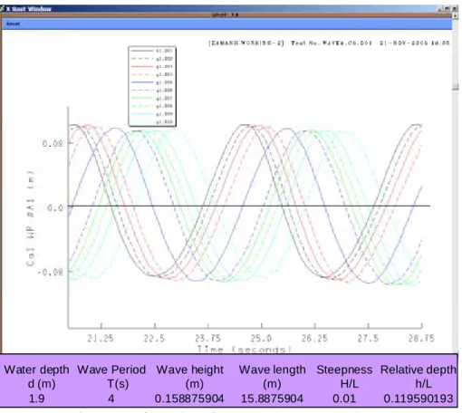
In the following analyses it is observed that when the wave frequency is less than 1/3 Hz then the wave data get contaminated very fast. That is, higher frequency wave takes longer time to build up the reflection. Figs. 3 to 6 show the wave propagations at Probe #1 to Probe #10 for the wave conditions shown in Table 2. It may be observed that the wave profiles are uniform and pretty close to each other in terms of their magnitude at all the wave probes locations except at those probes, which are close to the beach. This is due to the contamination of the reflected wave. As the wave period increases the wavelength and shallowness increases and thus the nonlinear and second order effects in the wave profile increases. In this experiment the acquired waves data with larger wave period got contaminated very fast.

Figs. 7 to 10 show the comparisons of the surface elevations obtained due to the Ist order wave generation technique, second order wave generation technique and those predicted by the code SPWNW.

Figs. 11 to 14 illustrate the energy flux density for the primary and the second order waves for parameters shown in Table 2 due to the second order wave generation technique.

(11)

Water depth Wave Period Wave height Wave length Steepness Relative depth

d (m) T(s) (m) (m) H/L h/L

1.9 2 0.06013907 6.013907 0.01 0.315934383

d (m) T(s) (m) (m) H/L h/L

1.9 2 0.06013907 6.013907 0.01 0.315934383

Fig. 3a Surface elevation at Probe #1 to Probe #10.

Water depth Wave Period Wave height Wave length Steepness Relative depth d (m) T(s) (m) (m) H/L h/L

1.9 2 0.12027814 6.013907 0.02 0.315934383 Water depth Wave Period Wave height Wave length Steepness Relative depth

d (m) T(s) (m) (m) H/L h/L 1.9 2 0.12027814 6.013907 0.02 0.315934383

(12)

d (m) T(s) (m) (m) H/L h/L

1.9 3 0.1111481 11.11481 0.01 0.170943093

d (m) T(s) (m) (m) H/L h/L

1.9 3 0.1111481 11.11481 0.01 0.170943093

Fig. 4a Surface elevation at Probe #1 to Probe #10.

Fig. 4b Surface elevation at Probe #1 to Probe #10.

d (m) T(s) (m) (m) H/L h/L

1.9 3 0.2222962 11.11481 0.02 0.170943093

d (m) T(s) (m) (m) H/L h/L

(13)

d (m) T(s) (m) (m) H/L h/L

1.9 4 0.158875904 15.8875904 0.01 0.119590193

Fig. 5a Surface elevation at Probe #1 to Probe #10

d (m) T(s) (m) (m) H/L h/L

1.9 4 0.317751808 15.8875904 0.02 0.119590193

Fig. 5b Surface elevation at Probe #1 to Probe #10

d (m) T(s) (m) (m) H/L h/L

(14)

Fig. 6a Surface elevation at Probe #1 to Probe #10

d (m) T(s) (m) (m) H/L h/L

1.9 5 0.204819832 20.4819832 0.01 0.092764455

Fig. 6b Surface elevation at Probe #1 to Probe #10

d (m) T(s) (m) (m) H/L h/L

(15)

Ist order generation

2nd order generation

Predicted by SPWNW

2nd

order generation

Predicted by SPWNW

Fig. 7a Comparisons of the surface elevations at Probe #1 to Probe #10

Water depth W tive depth

d (m) T(s) (m) (m) H/L h/L ave Period Wave height Wave length Steepness Rela

Water depth W tive depth

d (m) T(s) (m) (m) H/L h/L ave Period Wave height Wave length Steepness Rela

(16)

Predicted by SPWNW

Fig. 7b Comparisons of the surface elevations at Probe #1 to Probe #10

Water depth Wave Period Wave height Wave length Steepness Relative depth d (m) T(s) (m) (m) H/L h/L Water depth Wave Period Wave height Wave length Steepness Relative depth

(17)

Predicted by SPWNW

2nd

order generation

Predicted by SPWNW

(18)

Predicted by SPWNW

2nd

order generation

Predicted by SPWNW

Water depth Wave Period Wave height Wave length Steepness Relative depth Water depth Wave Period Wave height Wave length Steepness Relative depth

(19)

Predicted by SPWNW

2nd

order generation

Predicted by SPWNW

(20)

2nd

order generation

Predicted by SPWNW

Water depth Wave Period Wave height Wave length Steepness Relative depth Water depth Wave Period Wave height Wave length Steepness Relative depth

(21)

Predicted by SPWNW

2 order generation

Predicted by SPWNW

nd

(22)

2nd

order generation

Predicted by SPWNW

2 order generation

Predicted by SPWNW

nd

(23)

Fig. 11a(P1) Energy density at probes #1 to #10 for primary waves

(24)

Fig. 11a(P2) Energy density at probes #1 to #10 for second order waves

1.9 2 0.06013907 6.013907 0.01 0.315934383

d (m) T(s) (m) (m) H/L h/L

1.9 2 0.06013907 6.013907 0.01 0.315934383

(25)

Fig. 11b(P1) Energy density at probes #1 to #10 for primary waves

(26)

Fig. 11b(P2) Energy density at probes #1 to #10 for second order waves

(27)

(28)

(29)

(30)

(31)

ater depth Wave Period Wave height Wave length Steepness Relative depth d (m) T(s) (m) (m) H/L h/L

1.9 4 0.158875904 15.8875904 0.01 0.119590193 W

(32)

(33)

(34)

(35)

(36)

(37)

ater depth Wave Period Wave height Wave length Steepness Relative depth d (m) T(s) (m) (m) H/L h/L

1.9 5 0.409639664 20.4819832 0.02 0.092764455 W

(38)

(39)

Conclusions

In this experiment the water depth was 1.9m and to generate a shallow water wave we had to choose larger wave period and the acquired data got contaminated due to the faster reflection from the beach.

To avoid this problem we have conducted similar experiments once again with physically shallow water depth (0.6m and 0.8m) and that have allowed us to use smaller wave periods to avoid massive reflection. The analyses of the obtained data are yet to be completed. When the analysis is completed then another report would be produced. Difficulties

The software used here is designed and coded by CHC. It is important to get this software properly fit with the OEB. This software is very big in size and took pretty long time to develop.

Acknowledgement

The authors highly acknowledge the help from Mike Sullivan and Shane Mckay of the Facilities Department at the Institute of Ocean Technology, National Research Council of Canada.

eferences

Barthel V., Mansard, E.P.D., Sand, S.E. and Vis, F.C. (1983), “Group bounded long waves in physical models”, Ocen Eng. 10(4).

Longuet-Higgins, M. S. and R. W. Stewart (1961): "The changes in amplitude of short gravity waves on steady non-uniform currents," J. Fluid Mech., Vol.10, pp.529-549. Longuet-Higgins, M. S. and R. W. Stewart (1962), "Radiation stress and mass transport in gravity waves with application to surf beats," J. Fluid Mech., Vol.13, pp.481.

Longuet-Higgins, M. S. and R. W. Stewart (1963), "A note on wave set-up," J. Marine

Res., Vol.21, pp.9.

Longuet-Higgins, M. S. and R. W. Stewart (1964), "Radiation stress in water waves, a physical discussion with application," Deep-Sea Res., Vol.11, pp.529.

Sand, S. E. (1982), ”Long wave problems in laboratory models”, Proceedings of the

ASCE, J. of Wway, Port, coast. And Ocn. Div. Vol. 198 (WW4).