Adaptive and Selective Time Averaging of Auditory Scenes

Adaptive and Selective Time Averaging of Auditory Scenes

The MIT Faculty has made this article openly available.

Please share

how this access benefits you. Your story matters.

Citation

McWalter, Richard and Josh H. McDermott, "Adaptive and Selective

Time Averaging of Auditory Scenes." Current Biology 28, 9 (May

2018): p. 1405-1418.e10 doi. 10.1016/j.cub.2018.03.049 ©2018

Authors

As Published

https://dx.doi.org/10.1016/J.CUB.2018.03.049

Publisher

Elsevier BV

Version

Author's final manuscript

Citable link

https://hdl.handle.net/1721.1/126271

Terms of Use

Creative Commons Attribution-NonCommercial-NoDerivs License

Adaptive and Selective Time-Averaging of Auditory Scenes

Richard McWalter1,2,*,+ and Josh H. McDermott2,3,*

1_{Department of Electrical Engineering, Technical University of Denmark, Kgs. Lyngby, 2800,}

Denmark

2_{Department of Brain and Cognitive Sciences, Massachusetts Institute of Technology, Cambridge,}

MA 02139, USA

3_{Program in Speech and Hearing Biosciences and Technology, Harvard University, Cambridge,}

MA 02138, USA

Summary

To overcome variability, estimate scene characteristics, and compress sensory input, perceptual systems pool data into statistical summaries. Despite growing evidence for statistical

representations in perception, the underlying mechanisms remain poorly understood. One example of such representations occurs in auditory scenes, where background texture appears to be

represented with time-averaged sound statistics. We probed the averaging mechanism using “texture steps” – textures containing subtle shifts in stimulus statistics. Although generally imperceptible, steps occurring in the previous several seconds biased texture judgments, indicative of a multi-second averaging window. Listeners seemed unable to willfully extend or restrict this window but showed signatures of longer integration times for temporally variable textures. In all cases the measured timescales were substantially longer than previously reported integration times in the auditory system. Integration also showed signs of being restricted to sound elements attributed to a common source. The results suggest an integration process that depends on stimulus characteristics, integrating over longer extents when it benefits statistical estimation of variable signals, and selectively integrating stimulus components likely to have a common cause in the world. Our methodology could be naturally extended to examine statistical representations of other types of sensory signals.

*_{Correspondence: mcwalter@mit.edu, jhm@mit.edu.}

+Lead Contact

Publisher's Disclaimer: This is a PDF file of an unedited manuscript that has been accepted for publication. As a service to our

customers we are providing this early version of the manuscript. The manuscript will undergo copyediting, typesetting, and review of the resulting proof before it is published in its final citable form. Please note that during the production process errors may be discovered which could affect the content, and all legal disclaimers that apply to the journal pertain.

Author Contributions Conceptualization & Methodology, R.M. and J.H.M.; Formal Analysis & Investigation, R.M.; Writing, R.M.

and J.H.M.; Funding Acquisition & Supervision, J.H.M.

HHS Public Access

Author manuscript

Curr Biol

Curr Biol. 2018 May 07; 28(9): 1405–1418.e10. doi:10.1016/j.cub.2018.03.049.

A

uthor Man

uscr

ipt

A

uthor Man

uscr

ipt

A

uthor Man

uscr

ipt

A

uthor Man

uscr

ipt

Introduction

Sensory receptors measure signals over short timescales, but perception often entails combining these measurements over much longer durations. In some cases, this is because the structures that we must recognize are revealed gradually over time. In other cases, the presence of noise or variability means that samples must be gathered over some period of time in order for quantities of interest to be robustly estimated. Although much is known about integration over space via receptive fields of progressively larger extent in the visual system [1, 2], less is known about analogous processes in time.

Integration plays a fundamental role in the domain of textures – signals generated by the superposition of many similar events or objects. In vision and touch, texture often indicates surface material (bark, grass, gravel etc.) [3]. In audition, textures provide signatures of the surrounding environment, as when produced by rain, swarms of insects, or galloping horses [4–7]. Whether received by sight, sound, or touch, textures are believed to be represented in the brain by statistics that summarize signal properties over space or time [8–11].

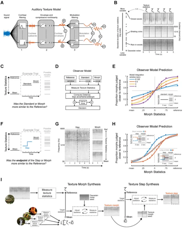
Statistical representations, in which signals are summarized with aggregate measures that pool information over space or time, are believed to contribute to many aspects of perception [2, 12–24], but texture is a particularly appealing domain in which to study them. Textures are rich and varied, ubiquitous in the world, relevant to multiple sensory systems, and arguably the only type of signal that is well described (at present) by biologically plausible models that are signal-computable (i.e., that operate on actual sensory signals and as such can be applied to arbitrary input; Figure 1A). Moreover, the proposed integration operation for texture is simple: the statistics believed to underlie texture perception can all be written as averages of sensory measurements of various sorts [5, 8]. In sound, this averaging occurs over time.

The goal of this paper was to characterize the extent and nature of the averaging mechanism. We posed three questions. First, is there a particular temporal extent over which averaging occurs? Second, does this extent depend on the intrinsic timescales of the signal being integrated? Third, is information averaged blindly within an integration window, or is it subject to perceptual grouping?

It was not obvious a priori what sort of averaging processes to expect. Longer term averages are more robust to variability and noise, but run the risk of pooling together signals with distinct statistical properties. Moreover, textures vary in the timescale at which they are stationary (i.e., at which they have stable statistics), reflected in the variability of their statistics (Figure 1B). Some textures, such as dense rain, have statistics that are stable over even short timescales, and that could be reliably measured with a short-term time-average. But others, such as ocean waves, are less homogeneous on local time scales despite being generated by a process with fixed long-term parameters. In the latter case, a longer averaging window might be necessary to accurately measure the underlying statistical properties. It thus seemed plausible that an optimal integration process would vary in the timescale of integration depending on the nature of the acoustic input. An additional complexity is that textures in real-world scenes typically co-occur with other sounds, raising the question of

A

uthor Man

uscr

ipt

A

uthor Man

uscr

ipt

A

uthor Man

uscr

ipt

A

uthor Man

uscr

ipt

whether texture statistics are averaged blindly over all the sound occurring within some window.

We developed a methodology to probe the averaging process underlying texture perception using synthetic textures whose statistics underwent a subtle shift at some point during their duration. The rationale was that judgments of texture should be biased by the change in statistics if the stimulus prior to the change is included in the average. By measuring the conditions under which biases occurred, we hoped to characterize the extent of averaging and its dependence on signal statistics and perceptual grouping.

Results

The logic of our main task was to measure the statistics ascribed to one texture stimulus by asking listeners to compare it to another (Figure 1C). The stimuli were intended to resemble natural sound textures and thus varied in a high-dimensional statistical space previously found to enable compelling synthesis of naturalistic textures [5, 7, 9]. To render the discrimination of such high-dimensional stimuli well-posed, we defined a line in the space of statistics between a mean texture stimulus and a reference texture and generated stimuli from different points along this line (that thus varied in their perceptual similarity to the reference texture). The reference texture was defined by the statistics of a particular real world texture; the “mean” texture was defined by the average statistics of 50 real-world textures. To familiarize listeners with the dimension of stimulus variation, the mean and reference stimulus were presented repeatedly prior to a block of trials based on the

reference. On each trial, they were asked to judge which of two stimuli was most similar to the reference. This design was chosen because presenting the reference on each trial would have produced prohibitively long trials.

To ensure that the task could be performed as intended using time-averaged statistics, we implemented an observer model (Figure 1D). The model measured statistics from each experimental stimulus using an averaging window extending for some duration from the end of the stimulus and chose the stimulus whose statistics were closest to those of the reference. Figure 1E shows the result of the model performing the task for a range of different

averaging window durations. The “standard” was fixed at the midpoint of the statistics continuum, whereas the “morph” varied from trial to trial between the reference and mean texture, never with the same statistics as the standard. Here and in the subsequent

experiments, the results are expressed as psychometric functions, plotting the proportion of trials on which the morph was judged closer to the reference as a function of the morph statistics.

As expected, the proportion of trials on which the morph was chosen increased as the morph statistics approached the reference, with the point of subjective equality at the midpoint on the statistic continuum (Figure 1E). This result confirms that the task can be performed using statistics measured from the stimuli but also that above-chance performance can be obtained for a range of window durations.

A

uthor Man

uscr

ipt

A

uthor Man

uscr

ipt

A

uthor Man

uscr

ipt

A

uthor Man

uscr

ipt

In order to assess the extent over which statistics were averaged by the human auditory system, we asked listeners to compare a texture whose statistics underwent a change mid-way through their duration (“steps”) to a texture whose statistics were constant (“morphs”; Figure 1F). Because the extent of integration was not obvious a priori, and because it was not obvious whether listeners would retain only the most recent estimate of the statistics of a signal, they were told that the first stimulus would undergo a change, and that they should base their judgments on the end of the stimulus. We envisioned that if listeners incorporated the signal preceding the step into their statistic estimate, the estimate would be shifted away from the endpoint statistics, biasing discrimination judgments. Figure 1G displays a spectrogram of an example texture step and three morphs for the “swamp insects” reference texture (see Figure S1 for visualizations of the statistic changes in step stimuli). In practice, we used several different reference textures per experiment, and the experiments were divided into blocks of trials based on a particular reference.

Figure 1H shows the result of the model performing the texture step discrimination task with two different averaging windows extending from the end of the stimulus. When the

averaging window included the step, the psychometric functions were shifted in the direction of the step, as intended. We tested whether human listeners would exhibit similar biases and, if so, over what timescales.

Textures were synthesized using an extended version of the McDermott and Simoncelli [5] sound synthesis procedure, in which Gaussian noise was shaped to have particular values for a set of statistics. Statistics were measured from a model of the peripheral auditory system that simulated cochlear and modulation filtering [25] (Figure 1A). The statistics employed included marginal moments and pairwise correlations measured from both sets of filters; each class of statistics is necessary for realistic texture synthesis [5] and thus is perceptually significant. Steps were generated by first synthesizing a morph for the starting values of the step statistics and then running the synthesis procedure again on the latter part of the signal to shift the statistics to the end values of the step (Figure 1I). This avoided stimulus discontinuities not necessitated by the change in statistics.

Although the stimuli were generated from target statistic values that underwent a discrete step, statistics must be measured over some temporal extent, and thus, the statistics

measured from a signal at different points in time inevitably exhibit a gradual transition from the value before the step to the value after the step (Figure S2). However, this gradual transition is strictly a consequence of averaging the stimulus before and after the step location – the stimulus itself was not biased by the step, as shown by the statistics measured by windows immediately adjacent to the step (Figure S2). Bias in perceptual judgments is thus diagnostic of the inclusion of the stimulus prior to the step.

Experiment 1: Step size selection

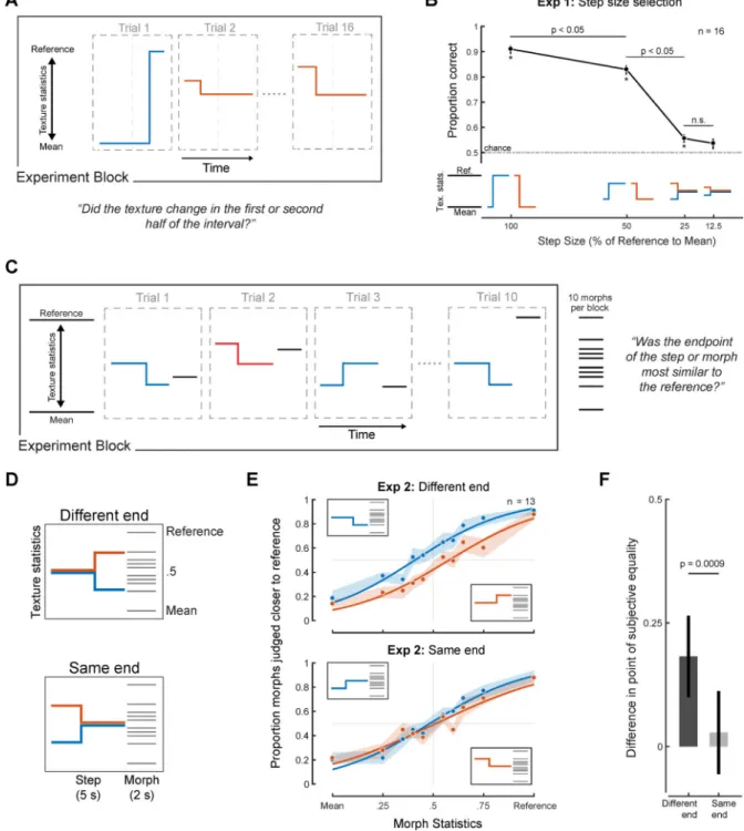
Because it seemed plausible that task performance might be affected by audible changes in the stimulus, we sought to use texture steps that were difficult to detect (but that were otherwise as large as possible, to elicit measurable biases). We conducted an initial experiment to determine an appropriate step size. Steps were generated in either the first or second half of a 5s texture stimulus, and listeners were asked to identify whether the step

A

uthor Man

uscr

ipt

A

uthor Man

uscr

ipt

A

uthor Man

uscr

ipt

A

uthor Man

uscr

ipt

occurred in the first or second half (Figure 2A). Steps of 25% were difficult to localize (Figure 2B), and this step magnitude was selected for use in subsequent step experiments. Experiment 2: Task validation

The other requirement of our experimental design was that listeners base their judgment on the end of the step interval. We evaluated compliance with the instructions by comparing discrimination for steps presented at either the beginning or end of the stimulus (Figure 2C&D). If listeners used the endpoint of the step interval as instructed, their judgments should differ substantially for the two different end conditions but less so for the two same end conditions, assuming the entire stimulus does not contribute to listeners’ judgments. As shown in Figure 2E, the psychometric functions for the different end conditions were offset, whereas those for the same end conditions were not. The offset in the psychometric functions was quantified as the difference in the point of subjective equality (Figure 2F), which was significantly different from zero for the Different End conditions (p < 0.0001, via bootstrap), but not for the Same End conditions (p = 0.15). These results suggest listeners were indeed able to follow the instructions and used the endpoint of the step interval when making judgments.

Experiments 3–5: Effect of stimulus history on texture judgments

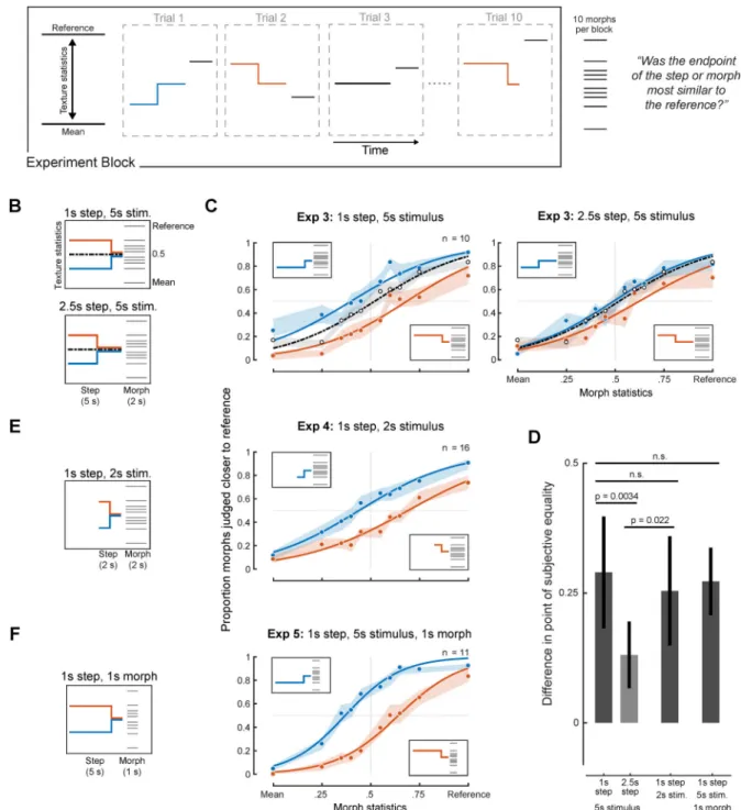
Having established that listeners could perform the task, we turned to the main issue of interest: the extent of the stimulus history included in texture judgments. As an initial assay we positioned the step at two different points in time (either 1s or 2.5s from the endpoint, Figure 3A&B). The step moved either toward or away from the reference, with an endpoint midway between the mean and reference texture. The experiment also included a baseline standard condition with constant statistics at the midpoint between the reference and mean texture, for which no bias was expected.

The baseline condition with constant statistics (black curve) yielded the expected psychometric function with a point of subjective equality at the midpoint of the statistic continuum (Figure 3C). By contrast, the psychometric functions for the step conditions were offset in either direction, indicating that the stimulus history beyond the step influenced listeners’ judgments despite the instructions to base their judgments on the step endpoint. The bias (again quantified as the difference in the point of subjective equality for the two step directions) was statistically significant for both the 1s steps (Figure 3D; p<0.0001; via bootstrap) and 2.5s steps (p<0.0001), but was significantly reduced in the latter condition (p=0.0034). The bias was also slightly asymmetric (greater for the red than blue curves, p<0.0001 for 2.5s step; see Figure S3 for bias measurements for individual step directions), suggesting that listeners incorporated more of the stimulus history for one step direction than the other. We will return to this latter issue in Experiment 7 and 8. Overall, however, the results are consistent with integration over the course of a few seconds.

Although one interpretation of the multi-second integration evident in Experiment 3 is that it reflects an obligatory perceptual mechanism, the results could also in principle be explained by a decision strategy. Two possibilities seemed particularly worth addressing. The first is that upon being instructed that the step stimulus would undergo a subtle change, listeners

A

uthor Man

uscr

ipt

A

uthor Man

uscr

ipt

A

uthor Man

uscr

ipt

A

uthor Man

uscr

ipt

may have assumed that the change would most likely happen mid-way through the stimulus, and accordingly listened to roughly the last half of the 5s stimulus when making their judgments. A second possibility was that listeners monitored the step stimulus for an extent comparable to the 2s duration of the morph stimulus to which the step was compared. Both of these strategies would have produced integration over several seconds in Experiment 3, but would predict different integration extents if stimulus duration was varied.

To explore whether listeners were simply monitoring the last half of the step stimulus, we repeated Experiment 3 with a two-second step stimulus with a step at 1s (Figure 3E). If listeners based judgments on the last half of the stimulus, the 1s step should yield similar results to the 2.5s step from Experiment 3. By contrast, if integration was due to a perceptual process that was largely independent of the stimulus duration, results should instead be similar to the 1s step from Experiment 3. As shown in Figures 3D & 3E, the bias from the 1s step in the two-second stimulus was indistinguishable from that of the 1s step in the five-second stimulus of Experiment 3 (p=0.51), and significantly different from that of the 2.5s step in Experiment 3 (p=0.022). These results are consistent with a perceptual mechanism of fixed extent rather than a decision strategy based on the stimulus duration.

To assess the effect of the morph duration we also repeated the 1s step conditions of Experiment 3 using a one-second morph stimulus (Figure 3F). The biases measured here were again indistinguishable from those measured with a comparison stimulus twice as long (p=0.76).

Both of these experiments indicate that the extent of the stimulus that influences texture judgments seems to be relatively independent of the stimulus durations. This is consistent with the idea that the averaging is perceptual in origin, and not strongly subject to strategies employed by the listener.

Experiment 6: Can integration be extended?

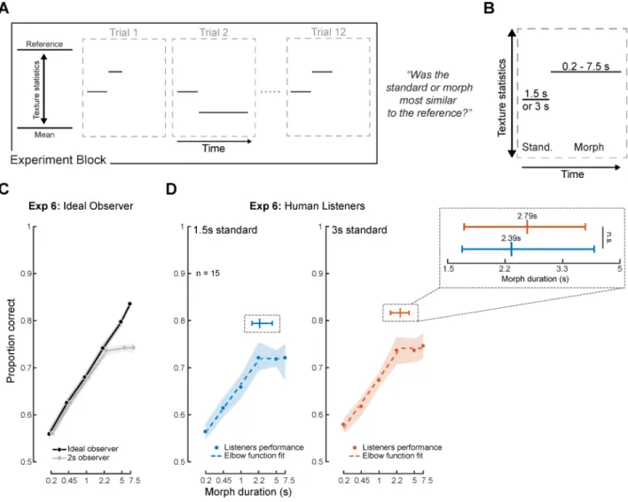
The results of Experiments 3–5 suggest that listeners integrate over several seconds to estimate texture statistics even when warned that the signals were changing and that they should attend to their endings. To further explore the extent to which integration was obligatory, we investigated whether listeners could instead extend integration when it would benefit performance. We designed an alternative task in which listeners were presented with two texture excerpts generated from constant statistic trajectories: a “standard” excerpt of a fixed duration, and a morph whose duration varied from 0.2 to 7.5 seconds and whose statistics could either be closer or further from the reference with equal probability (Figure 4A&B). Listeners again judged which of the two sounds was more similar to a reference texture, and the sounds were again generated from statistics drawn from the line between the mean and reference statistics.

We reasoned that statistical estimation should benefit from averaging over the entire morph duration, such that an ideal observer would improve continuously as the duration increased (Figure 4C, black curve). But if listeners were constrained by an integration window of fixed duration and retained only its most recent output for a given stimulus, performance might be expected to plateau after the probe duration exceeded it (Figure 4C, gray curve). We used

A

uthor Man

uscr

ipt

A

uthor Man

uscr

ipt

A

uthor Man

uscr

ipt

A

uthor Man

uscr

ipt

two different standard durations (1.5 and 3 seconds, fixed within blocks) to verify that integration over the morph was not somehow determined by the duration of the sound it was being compared to. A fixed standard duration was used to avoid prohibitively long trials, which would otherwise have occurred if both stimuli varied in duration.

As shown in Figure 4D, performance increased with duration of the morph interval up to 2 seconds, but then plateaued, with no improvement for the longest two durations used. Results were similar for both standard durations. We assessed the location of the plateau by fitting an elbow function [26] to the data, bootstrapping to obtain confidence intervals on the elbow point (Figure 4D, top inset). The best-fitting elbow points were 2.39 and 2.79s (for 1.5s and 3s standards, respectively, which were not significantly different, p=0.96). This finding is consistent with the idea that listeners cannot average over more than a few

seconds, at least for the textures we used here, even when it would benefit their performance. The results provide additional evidence for a perceptual integration mechanism whose temporal extent is largely obligatory and not under willful control.

Experiments 7 & 8: Effect of texture variability on temporal integration

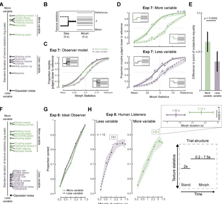
Although Experiments 3–6 were suggestive of an averaging mechanism whose temporal extent was relatively fixed, there was some reason to think that integration might not always occur over the same timescale. In particular, optimal estimation of statistics should involve a tradeoff between the variability of the estimator (which decreases as the integration window lengthens) and the likelihood that the estimator pools across portions of the signal with distinct statistics (which increases as the integration window lengthens). Because textures vary in their stationarity, the window length at which this tradeoff is optimized should also vary. For highly stationary textures, such as dense rain, a short window might suffice for stable estimates, whereas for less stationary textures, such as the sound of ocean waves, a longer window could be better. We thus explored whether the timescale of integration might vary according to the variability of the sensory signal.

We first evaluated the variability of a large set of textures by measuring the variation in statistics measured in 1s analysis windows (Figure 5A). We selected the six textures with maximum variability and the six with minimum variability for use as reference textures in an experiment. We then repeated the step discrimination paradigm of Experiment 3 with a step at 2.5s (Figure 5B).

To underscore the fact that integration times need not be different for the two sets of textures, we ran our observer model on the experiment using a single fixed analysis window (of 3s). The model yielded similar biases for both texture sets (Figure 5C; see Figure S4 for comparable results with other window durations). It was thus plausible that human listeners might also exhibit comparable biases for the two sets of stimuli.

Unlike the model results obtained with a fixed averaging window, the bias in human listeners was substantially larger for the textures that were more variable (p = 0.0002, Figure 5D&E). This result suggests that more of the stimulus history is incorporated into statistic estimates for the more variable textures, and is consistent with an averaging process whose temporal extent is linked to the temporal variability of the texture. It also appears that the degree of

A

uthor Man

uscr

ipt

A

uthor Man

uscr

ipt

A

uthor Man

uscr

ipt

A

uthor Man

uscr

ipt

bias for the more homogeneous textures is greater than that observed in Experiment 3 for the 2.5s condition (non-significant trend: p = 0.087). Although the participants were different between experiments, this difference could indicate that the extent of averaging adapts to the local context, such that the presence of highly variable textures within the experiment could affect the extent of averaging in the blocks with less variable textures.

As a further test of the effect of texture variability, we conducted a second experiment, in this case replicating the design of Experiment 6, again using two sets of textures that clustered at opposite ends of the spectrum of variability (Figure 5F). An ideal observer model produced similar results for the two sets of textures (Figure 5G), but human listeners did not: the dependence of performance on the probe duration was different for the two groups of textures, with discrimination appearing to plateau at a longer probe duration for the more variable textures (Figure 5H). To quantify this effect, we again fit piecewise linear “elbow” functions to the data (Figure 5H, top inset). The elbow points of the best fitting functions were 1.42s and 3.16s for the less and more variable textures, respectively, and were significantly different (p=0.0043, via bootstrap).

This finding replicated when the results of Experiment 6 were re-analyzed, splitting the textures into more and less variable groups. Even though these textures were distinct from those of Experiment 8, and were not selected for their statistic variability, it was again the case that discrimination performance plateaued at longer durations for more variable textures (Figure S5). Longer integration for more variable textures is also consistent with the asymmetric results in Experiment 3 (in which history-induced biases were larger for steps in one direction than the other). As shown in Figure S2, the statistics of the step closer to the reference were more variable than those of the step closer to the mean (larger error bars for the red compared to the blue curve, due to the reference textures in that experiment being more variable than the mean texture). No such asymmetry is evident in Experiment 7, but that may be because the differences across textures were much larger than in Experiment 3, swamping any effect of the step direction.

Overall, the results provide converging evidence for an averaging process that pools information over a temporal extent that depends on the signal variability.

Experiment 9: Effect of stimulus continuity on texture integration

The apparent presence of an averaging window raised the question of whether the

integration process operates blindly over all sound that occurs within the window, or whether integration might be restricted to the parts of the sound signal that are likely to belong to the same texture. We explored this issue by introducing audible discontinuities in the step stimulus immediately following the statistic change. We hypothesized that the discontinuity might cause the history prior to it to be excluded from or down-weighted in the averaging process.

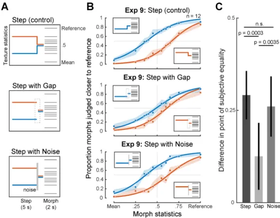
We created three variants with a step positioned 1s from the endpoint (Figure 6A). The first condition preserved continuity at the step (as in Experiment 3), whereas the second condition replaced the texture immediately following the step with a silent gap (200ms in duration). A third condition tested the effect of perceptual rather than physical continuity by

A

uthor Man

uscr

ipt

A

uthor Man

uscr

ipt

A

uthor Man

uscr

ipt

A

uthor Man

uscr

ipt

filling the gap with a spectrally matched noise burst that was substantially higher in intensity than the texture, causing the texture to sound continuous [27, 28]. Listeners were again instructed to base their judgments on the endpoint of the step stimulus.

As shown in Figure 6B, the gap (middle panel) substantially reduced the bias produced by the step compared to the continuous (top panel) or noise burst (bottom panel) conditions. This reduction was statistically significant in both cases (gap versus continuous: p = 0.0003; gap versus noise burst: p = 0.0035; Figure 6C). By contrast, the biases measured for the continuous step and noise burst conditions were not significantly different (p = 0.46). These results are consistent with the idea that the integration process underlying texture judgments is partially reset by discontinuities attributed to the texture but not by those attributed to other sources, as though integration occurs preferentially over parts of the sound signal that are likely to have been generated by the same process in the world.

Experiment 10: Effect of foreground/background on texture grouping

The finding that integration appears to occur across an intervening noise burst (Experiment 9) raised the question of whether such extraneous sounds are included in the texture integration process. Textures in auditory scenes are often superimposed with other sound sources, as when a bird calls next to a stream, or a person speaks during a rainstorm. Are such sounds excluded from the integration process?

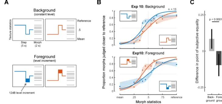
To test whether foreground sounds embedded in a texture are excluded from integration, we extended our texture step paradigm. Stimuli were generated with three segments (producing two steps, at 2s and 1s from the endpoint). In the “Background” condition, the segments were all the same intensity and appeared to all be part of the same continuous background texture (Figure 7A, top panel). In the “Foreground” condition, the level of the second segment was 12dB higher than the other segments (Figure 7A, bottom panel). The level increment caused the middle segment to perceptually segregate from the other two segments, which were heard as continuing through it [27, 28]. The segment statistics were chosen such that integration over several seconds would yield biases in opposite directions depending on whether the middle segment was included in the integration, as confirmed with observer models that integrated blindly or that excluded the middle segment (Figure S6). Listeners were told that the step interval might undergo a change in loudness, and that they should in all cases base their judgments on the endpoint of the step stimulus.

Without the level increment, listeners’ judgments exhibited a bias toward the statistics of the middle segment (Figure 7B, top), consistent with its inclusion in the averaging process used to estimate texture statistics. However, the bias was reversed when the middle segment was higher in level than its neighbors (Figure 7B, bottom; the biases in the two conditions were significantly different: p<0.0001, Figure 7C). This pattern of results is consistent with what would be expected if the middle segment was excluded from the integration, and if

integration extended across the middle segment to include part of the first segment (consistent with Experiment 9). These results provide further evidence that texture

integration is restricted to sounds that are likely to have come from a similar source. Overall, the results of Experiments 9 and 10 indicate that texture perception functions as part of auditory scene analysis, concurrent with the grouping or streaming of sound sources.

A

uthor Man

uscr

ipt

A

uthor Man

uscr

ipt

A

uthor Man

uscr

ipt

A

uthor Man

uscr

ipt

Discussion

Textures, be they visual, auditory, or tactile, are believed to be represented with statistics – averages over time and/or space of sensory measurements. We conducted a set of

experiments on sound textures to probe the nature of the averaging process. We found that the judgments of human listeners were biased by subtle changes in statistics that occurred in the previous several seconds, implicating an integration process over this extent

(Experiments 3–5). This effect was present even though participants were instructed to attend to the end of the stimulus and were warned that the stimulus would undergo changes. When given the opportunity to average over more than a few seconds (Experiment 6), listeners did not appear able to do so. However, the biasing effects of the stimulus history were more pronounced when textures were more variable, suggesting that the integration process occurs over longer extents in the presence of higher stimulus variability, perhaps as needed to achieve stable statistic estimates (Experiment 7 & 8). We also found that biasing effects were diminished when there was a salient change (silent gap) in the texture (Experiment 9), as though the integration process partially resets itself in such conditions. Lastly, texture integration appears to occur across foreground sounds that interrupt a texture (Experiment 9), but to exclude such foreground sounds from the calculation of the texture’s statistics (Experiment 10). The results indicate an integration process extending over several seconds that compensates for the temporal complexity of the auditory input, and that appears to be inseparable from auditory scene analysis.

Evidence for perceptual integration

One natural question is whether these effects might be attributed to a cognitive decision strategy on the part of the listener rather than a perceptual mechanism. There was some reason a priori to think that listeners would be constrained to base their judgments on time-averaged statistics – previous experiments suggest that listeners can discriminate texture statistics, but not the details that give rise to those statistics [9]. We employed textures taken from those prior studies, and used similar stimulus durations, making it likely that listeners were similarly limited to statistical judgments in our tasks. However, listeners might in principle be able to control the temporal extent over which statistics were computed depending on the stimulus and task, in which case the integration extent would reflect their strategy rather than the signature of a perceptual mechanism.

Several lines of evidence suggest that this is not the case. First, listeners were told to base their judgments on the end of the step stimulus, and did so (Experiment 2), but were nonetheless biased by stimulus features several seconds in the past. Moreover, the extent of integration appeared to be approximately invariant to stimulus duration (Experiment 4), and to the duration of the comparison stimulus (Experiment 5), even though these manipulations might have been expected to cause listeners to adjust the extent of integration were it under willful control. Second, in a distinct experiment paradigm, listeners were unable to integrate over longer periods of time even when it would have benefitted their performance

(Experiments 6 and 8). This limitation is suggestive of a mechanism that constrains the information accessible to listeners. Moreover, the integration extent evident in these latter experiments was roughly comparable to that suggested by the step experiments

A

uthor Man

uscr

ipt

A

uthor Man

uscr

ipt

A

uthor Man

uscr

ipt

A

uthor Man

uscr

ipt

(Experiments 3–5 and 7) even though different integration strategies would have been optimal for each experiment. The fact that a similar integration timescale emerged from two different types of experiment gives support to a single sensory process that limits texture judgments.

One consequence of multi-second, obligatory integration is that sensitivity to changes in statistics should be limited – an averaging window blurs together the statistics on either side of a change. Experiment 1 provided evidence that this was the case for the steps that we used: listeners could not localize the step to one half of the stimulus or the other. We performed an additional experiment in which listeners simply had to detect the presence of a step at the stimulus midpoint. Results were comparably poor provided steps were modest in amplitude (Figure S7). The detection of larger steps might leverage salient signal

discontinuities that accompany pronounced statistic changes. Consistent with this notion, performance improved when a gap was inserted at the step location (Figure S7; see also Experiment 9).

The perception of stimuli longer than the texture integration window merits further exploration. Do listeners retain any sense of drift in statistical properties when they change over time [29]? One presumptive advantage of a limited averaging window is to retain some sensitivity to such changes. We know that listeners can retain estimates of texture statistics for multiple discrete excerpts, because they must in order to perform the discrimination tasks used here and elsewhere [9]. But it also appears that listeners do not always retain distinct estimates from different time points within the same statistical process (otherwise they would have shown some improvement with duration beyond a few seconds in Experiment 6) [30]. It thus remains to be seen how the temporal evolution of a changing statistical process is represented.

Effects of variability on time-averaging

Although the integration process underlying listeners’ judgments appeared not to be subject to willful control, its temporal extent showed signs of depending on the stimulus variability. One possibility is that different statistics have different integration times, and that different statistics are used for discrimination depending on the texture. For instance, more variable textures tend to have more power at slow modulations, which are plausibly measured over longer timescales than faster modulations [31]. Under this account, the variation in integration extent suggested by our experiments need not reflect an active process of adaptation to stimulus variability. One piece of evidence that appears inconsistent with this idea is that the bias for less variable textures in Experiment 7 was somewhat greater than that in Experiment 3, potentially because the most variable textures influenced integration on other blocks of trials. It thus remains possible that stimulus variability is sensed (e.g. by monitoring the stability of internal statistic estimates), and that it influences the extent of integration for individual statistics. Regardless of the mechanism, the effects of variability on integration suggest a potential general principle for time-averaging that could be present in other domains where statistical representations are used [14–21, 23, 24].

A

uthor Man

uscr

ipt

A

uthor Man

uscr

ipt

A

uthor Man

uscr

ipt

A

uthor Man

uscr

ipt

Temporal integration in the auditory system

Although our experiments represent the first attempt (to our knowledge) to measure an integration window for texture, there has been longstanding interest in temporal integration windows for other aspects of hearing. Loudness integration is perhaps most closely analogous to the averaging that seems to occur for texture, and is believed to reflect a nonlinear function of stimulus intensity averaged over a window of a few hundred milliseconds [32–35]. Integration also occurs in binaural hearing, on a similarly short timescale [36]. The integration process we have characterized for sound texture seems noteworthy in that it is quite long relative to typical timescales in the auditory system (though it is comparable to integration times proposed in parts of the visual system) [37]. We use the term integration here to refer specifically to averaging operations. In this respect the phenomena we study appear distinct from other examples in which prior context can change the interpretation of a stimulus [38–41]. In most such cases the representation of the current stimulus remains distinct from that of the past, and the effects seem better described either by history-dependent changes to the stimulus encoding (e.g. via adaptation) and/or by inference performed on the current stimulus with respect to the distribution of prior

stimulation [42, 43]. Such prior distributions can be learned over substantial periods of time, and in this respect appear distinct from texture representations, which represent the

momentary statistics of a sound source by averaging over a local temporal neighborhood. It is plausible that similar contextual effects occur with texture, i.e. that the longer-term statistical history [44] influences statistical estimates of the current stimulus state.

Apart from the (substantial) interactions with scene analysis phenomena (Experiments 9 and 10), our results are well described by a simple averaging window operating on a biologically plausible auditory model (Fig. S6). However, the averaging time scales implicated by our experiments are quite long relative to receptive fields in the auditory cortex (which are rarely longer than a few hundred milliseconds) [45–47]. To our knowledge the only phenomenon in the auditory system that extends over multiple seconds is stimulus-specific adaptation [44, 48–53]. Adaptation is widespread in sensory systems, and may also scale with stimulus statistics [54] but its computational role remains unclear. Whether adaptation could serve to compute quantities like texture statistics is an intriguing question for future research. Although we have suggested an averaging “window” of several seconds, we still know little about the shape of any such window. Systematic exploration of the effects of steps at different time lags could help to determine whether different parts of the signal are weighted differently. And as noted above, there need not be a single window – texture is determined by many different statistics, some of which might pool over longer windows than others, potentially depending on their intrinsic variability. Our results suggest a rough overall integration time constant of several seconds, but this could represent the net effect of different integration windows for different statistics. This issue could be investigated by generating steps that are restricted to particular statistics. We also note that the apparent sophistication of the averaging (excluding distinct foreground sounds, for instance) renders the metaphor of a “window” limited as a description of the integration process.

A

uthor Man

uscr

ipt

A

uthor Man

uscr

ipt

A

uthor Man

uscr

ipt

A

uthor Man

uscr

ipt

Texture perception and scene analysis

Our results indicate that texture integration is intertwined with the process of segregating an auditory scene into distinct sound sources. We found that a silent gap was sufficient to substantially reduce the influence of the stimulus history, suggestive of an integration process that selectively averages those stimulus elements likely to be part of the same texture. We also found evidence that concurrent foreground sounds are not included in the estimate of texture statistics when there is strong evidence that they should be segregated from the texture. Texture integration thus seems to be restricted to texture “streams”, which may be critical for accurate perception of textures in real-world conditions with multiple sound sources.

Relation to statistical representations in other sensory modalities

The results presented here seem likely to have analogs in statistical representations in other modalities [14–20, 24]. Visual texture representation is usually conceived as resulting from averages over spatial position [10, 11], but similar computational principles could be present for spatial averaging. Visual textures also sometimes occur over time, as when we look at leaves rustling in the wind [55], and the time-averaging evident with sound textures could also occur in such cases [16]. Tactile textures, where spatial detail is typically registered by sweeping a finger over a surface, also involve temporal integration [56, 57], the basis of which remains uncharacterized. In all these cases, the experimental methodology developed here could be used to study the underlying mechanisms.

STAR Methods

CONTACT FOR REAGENT AND RESOURCE SHARING

Further information and requests for resources and reagents should be directed to and will be fulfilled by the Lead Contact, Richard McWalter (mcwalter@mit.edu).

EXPERIMENTAL MODEL AND SUBJECT DETAILS

Participants were recruited from a university job posting site and had self-reported normal hearing. Experiments were approved by the Committee on the Use of Humans as

Experimental Subjects at the Massachusetts Institute of Technology. Participants completed the required consent form (overseen by the Danish Science-Ethics Committee or the

Committee on the Use of Humans as Experimental Subjects at the Massachusetts Institute of Technology) and were compensated with an hourly wage for their time. Participant

demographics were slightly different for each experiment and are provided below in sections for each experiment.

METHOD DETAILS

Auditory Texture Model—To simulate cochlear frequency analysis, sounds were filtered into subbands by convolving the input with a bank of bandpass filters with different center frequencies and bandwidths. We used 4th-order gammatone filters as they closely

approximate the tuning properties of human auditory filters and, as a filterbank, can be designed to be paraunitary (allowing perfect signal reconstruction via a paraconjugate

A

uthor Man

uscr

ipt

A

uthor Man

uscr

ipt

A

uthor Man

uscr

ipt

A

uthor Man

uscr

ipt

filterbank). The filterbank consisted of 34 bandpass filters with center frequencies defined by the equivalent rectangular bandwidth (ERBN) scale [59] (spanning 50Hz to 8097Hz). The

output of the filterbank represents the first processing stage from our model (Figure 1A). The resulting “cochlear” subbands were subsequently processed with a power-law compression (0.3) which models the non-linear behavior of the cochlea [60]. Subband envelopes were then computed from the analytic signal (Hilbert transform), intended to approximate the transduction from the mechanical vibrations of the basilar membrane to the auditory nerve response. Lastly, the subband envelopes were downsampled to 400Hz prior to the second processing stage.

The final processing stage filtered each cochlear envelope into amplitude modulation rate subbands by convolving each envelope with a second bank of bandpass filters. The modulation filterbank consisted of 18 half-octave spaced bandpass filters (0.5 to 200Hz) with constant Q = 2. The modulation filterbank models the selectivity of the human auditory system and is hypothesized to be a result of thalamic processing [25, 45, 61]. The

modulation bands represent the output of the final processing stage of our auditory texture model.

The model input was a discrete time-domain waveform, x(t), usually several seconds in duration (~5s). The texture statistics were computed on the cochlear envelope subbands, xk(t), and the modulation subbands, hk,n(t), where k indexes the cochlear channel and n

indexes the modulation channel. The windowing function, w(t), obeyed the constraint that

Σtw(t) = 1.

The envelope statistics include the mean, coefficient of variance, skewness and kurtosis, and represent the first four marginal moments. The marginal moments capture the sparsity of the time-averaged subband envelopes. The moments were defined as (in ascending order)

μk =∑_t w(t)xk(t) σk2 μk2= ∑tw(t)(xk(t) − μk)2 μk2 , ηk =∑tw(t)(xk(t) − μk)3 σk3 , Kk =∑tw(t)(xk(t) − μk)4

σk4 , k ∈ [1…34] in each case .

A

uthor Man

uscr

ipt

A

uthor Man

uscr

ipt

A

uthor Man

uscr

ipt

A

uthor Man

uscr

ipt

Pair-wise correlations were computed between the eight nearest cochlear bands. The correlation captures broadband events that would activate cochlear bands simultaneously [5, 62]. The measure can be computed as a square of sums or in the more condensed form can be written as

cjk =∑tw(t)(xj(t) − μj)(xk(t) − μk)_{σ jσk} , j, k, ∈ [1…34]

such that (k − j) = [1, 2, 3, 4, 5, 6, 7, 8] .

To capture the envelope power at different modulation rates, the modulation subband variance normalized by the corresponding total cochlear envelope variance was measured. The modulation power (variance) measure takes the following form

σk,n =∑tw(t)(bk,n(t) − μk,n)

2

σk2 , k ∈ [1…34], n ∈ [1…18] .

Lastly, the texture representation included correlations between modulation subbands of distinct cochlear channels. Some sounds feature correlations across many modulation subbands (e.g. fire), whereas others have correlations only between a subset of modulation subbands (ocean waves and wind, for instance, exhibit correlated modulation at slow but not high rates [5]). These correlations are given by

cjk,n =∑tw(t)(bj,n(t) − μj,n)(bk,n(t) − μk,n)_{σ j,nσk,n} ,

j ∈ [1…34], (k − j) = [1, 2], n ∈ [3 5 7 9 11 13] .

The texture statistics identified here resulted in a parameter vector, ζ, which was used to generated the synthetic textures.

Texture Stimuli Synthesis—Synthetic texture stimuli were generated using a variant of the McDermott and Simoncelli (2011) synthesis system. The synthesis process allowed for the generation of distinct exemplars that possessed similar texture statistics by seeding the synthesis system with different samples of random noise. The original system was modified (Figure 1I) to facilitate the generation of “texture morphs” (sound textures generated from statistics sampled at points along a line between two textures) and “texture steps” (sound textures that underwent a change in their statistics at some point during their duration). First, sound texture statistics were measured from 7-s excerpts of real-world texture recordings. The measured statistics comprised the mean, coefficient of variation, skewness, and kurtosis of the Hilbert envelope of each cochlear channel, pair-wise correlations across

A

uthor Man

uscr

ipt

A

uthor Man

uscr

ipt

A

uthor Man

uscr

ipt

A

uthor Man

uscr

ipt

cochlear channels, the power from a set of modulation filters, and pair-wise correlations across modulation bands [5]. Statistics were measured from 50 real-world texture recordings (Table S1). Statistics from individual real-world recordings, ζref were used to synthesize

“reference” textures. The statistics of all 50 recordings were averaged to yield the statistics,

ζmean, from which the “mean” texture was synthesized. In practice the envelope mean

statistics for the mean texture were replaced with those of the reference texture in order to avoid spectral discontinuities in the texture step stimuli. The measured statistics were imposed on a random noise seed whose duration depended on the stimulus type.

Texture morphs were generated by synthesizing a texture from a point along a line in the space of statistics between the mean and the reference (ζΔ1 = Δ1ζref + (1 − Δ1)ζmean), using

Gaussian noise as the seed.

Texture steps were generated such that their statistical properties changed at some point in time by stepping from one set of texture statistics to another. The process began by

synthesizing a texture from one set of statistics, ζΔ1, usually set to a point along a line in the

space of statistics between the mean and the reference (ζΔ1 = Δ1ζref + (1 − Δ1)ζmean), using

Gaussian noise as the seed. We then passed the synthesis system a second set of statistics, typically a different point along the same line in the space of statistics, ζΔ2, and the previous

synthetic texture as the seed. The two resulting synthetic textures were then windowed (with rectangular windows) and summed to create a texture step with the transition in the desired location. This synthesis process minimized artifacts that might otherwise occur by simply concatenating texture segments generated from distinct statistics – the seeding procedure helped ensure that the degree and location of amplitude modulations at the border between segments with distinct statistics were compatible. We were thus able to generate textures whose statistics varied over time, yet had no obvious local indication of the change in statistics. In practice the changes in the statistics were difficult to notice (as demonstrated in Experiments 1 and 11). Moreover, this approach ensured that the statistics on either side of the step were unbiased by the signal on the other side, as verified in Figure S2.

Texture Metric—Our stimulus generation and modeling assumed a Euclidean metric for each statistic class. We adopted this metric because discovering the perceptually correct metric seemed likely to be intractable given the high dimensionality of the statistic space. The metric we used seemed like the simplest possibility a priori, and so we used it in pilot psychophysical experiments. These pilot experiments suggested that stimuli spaced regularly according to a Euclidean metric produce pretty reasonable psychometric functions, and that texture steps in opposite directions that were equal-sized according to a Euclidean metric produced approximately equal biases (though not always, as is evident in Experiment 3). This suggests that even though the metric we used is surely not exactly right, it was sufficient for our purposes.

Observer Model—We created an observer model to quantify the effect of an integration window on texture discrimination. The model instantiated the hypothesis that stimuli are discriminated by comparing statistics computed by averaging nonlinear functions of the sound signal over some temporal window. We emphasize that the model was stimulus-computable – it operated on the actual sound waveforms used as experimental stimuli.

A

uthor Man

uscr

ipt

A

uthor Man

uscr

ipt

A

uthor Man

uscr

ipt

A

uthor Man

uscr

ipt

The model (Figure 1D) measured the texture statistics of the two stimuli in each trial of the experiment using an averaging window extending backward in time for some duration that was applied to the output of the auditory model described above. The model compared these measured statistics to the statistics of the reference texture (measured in the same way from a 5s sound waveform). The step and morph stimuli were generated from statistics on the line between the mean and reference texture statistics, but because the observer model computed statistics over finite windows, the measured statistics were always displaced from the line to some extent due to measurement error from the finite sample. To determine which stimulus was closer to the reference, the statistics of the step (ζ⃗step) and morph (ζ⃗morph) were thus

projected onto the line between the statistics of the mean (ζ⃗mean, also measured from a 5s

waveform) and reference (ζ⃗ref) texture:

ζ ref,i′ _{= ζ ref,i − ζ mean,i}

ζ step,i′ _{= ζ step,i − ζ mean,i}

ζ step,i″ = ζ step,i′

T ζ ref,i′

ζ ref,i′ T_{ζ ref,i}′ ζ ref,i,

ζ morph,i′ _{= ζ morph,i − ζ mean,i}

ζ morph,i″ = ζ morph,i′

T ζ ref,i′

ζ ref,i′ T_{ζ ref,i}′ ζ ref,i,

where i denotes the class of texture statistics (mean, coefficient of variation, skew, kurtosis, cochlear correlation, modulation power, modulation correlation).

Because the different classes of statistic (envelope mean, variance, skewness, and kurtosis; cross-envelope correlation; modulation power; cross-band modulation correlation) have different units and cover different ranges, the procedure described above was performed separately for each class, each time normalizing by the distance of the reference to the mean (ζ_{ref , i}′ ) for that statistic class. The mean and reference texture statistics were always substantially different (in part because they were always fairly high-dimensional), such that we never observed stability issues with this normalization process. These normalized distances were then summed across classes as follows:

A

uthor Man

uscr

ipt

A

uthor Man

uscr

ipt

A

uthor Man

uscr

ipt

A

uthor Man

uscr

ipt

dstep =1L∑_i ∑k |ζref,i,k

′ _{− ζstep,i,k}" |2 1/2 ∑k |ζref,i,k − ζmean,i,k|2 1/2+ ni,

dmorph =L1∑_i ∑k |ζref,i,k

′ _{− ζmorph,i,k}" |2 1/2 ∑k |ζref,i,k − ζmean,i,k|2 1/2 + ni,

where d is the distance to the reference texture statistics (ζ_{ref , i}′ ), i is the statistic class, L is the number of statistic classes, k indexes over statistics within a class, and n was Gaussian noise added to match the observer model’s overall performance to that of human listeners. The model then chose the smaller of the two distances {dstep, dmorph}.

The amplitude of the added noise was selected by averaging the behavioral data from many 1s step conditions (because we had the most data for this condition) across experiments (N=41 participants in total) and fitting the observer model’s psychometric function. The noise affected the slope of the psychometric function, but not the bias, and thus did not directly affect the main quantity of interest. The decision to weight each statistic class equally was arbitrary, but respected previous findings that each statistic class contributes to texture judgments [5].

To evaluate optimal performance characteristics for the duration experiment (Figure 4C), we implemented a related ideal observer model. The structure of the ideal observer was similar to the observer model described above, with the exception that the ideal observer operated on the entire length of the experimental stimulus, and that the statistics of the reference and mean texture were measured from 7.5s excerpts, equal to the longest morph duration. Experiments 9 (effect of noise burst and silent gap) and 10 (exclusion of foreground elements from texture integration) utilized stimuli with large signal discontinuities and thus necessitated a modified observer model to ensure that the measured statistics could be projected onto a line between the reference and mean texture. The observer model included a standard automatic gain control (AGC) to adjust the level of the incoming signal [63]. The AGC operated on the cochlear envelopes of the auditory texture model and adjusted their level to that of the reference texture. The cochlear envelope level was adjusted with a time-varying gain that depended on the signal level estimated over a local time window:

yk(t) = gk(t)xk(t), where gk(t) = gk,target/xk,avg(t)

where yk(t) is the envelope of the kth cochlear channel following gain control, xk(t) is the

envelope of the kth cochlear channel prior to gain control, gk is the gain, gk,target is the target

level (the mean of the reference texture envelope), and xk,avg(t) is the cochlear envelope

amplitude averaged over a local time window:

A

uthor Man

uscr

ipt

A

uthor Man

uscr

ipt

A

uthor Man

uscr

ipt

A

uthor Man

uscr

ipt

xk,avg(t) = [1 − α]xk,avg(t − 1) + αxk(t),

where α determines the extent of averaging over time (α = 20 · ΔT, where ΔT is the sample period, which was 2.5ms in our implementation).

The AGC prevented the large differences in level produced by the 12dB increment of the foreground condition from dominating the statistical measurements. The observer model was also modified to analyze only the portions of the step interval with non-zero values (to prevent the level differences introduced by the gap from dominating the statistical

measurements). This was implemented with a window function in each statistical measurement that applied positive weight only to non-zero portions of the signal. We compared this “blind” observer model (which measured statistics from all non-zero portions of the signal falling within a fixed integration window of 2.5s) to an “oracle” model. The oracle model averaged statistics over only selected portions of the signal specified by the experimenter as those potentially selected as belonging to the same sound source (indicated by the gray regions in the insets of the right column of Figure S6). We emphasize that only the “blind” model was signal-computable; the oracle model required the specification of the signal segments to be averaged. The oracle model is included only to demonstrate that selective averaging could produce the observed experimental results were there a way to implement the selection.

Experimental Procedures – Sound Presentation—The Psychophysics Toolbox for MATLAB [58] was used to play sound waveforms. All stimuli were presented at 70 dB SPL with a sampling rate of 48 kHz in a soundproof booth (Industrial Acoustics). For

experiments conducted at MIT, sounds were played from the sound card in a MacMini computer over Sennheiser HD280 PRO headphones. For experiments conducted at DTU, sounds were played from an RME FireFace UCX sound card over Sennheiser HD650 headphones.

Experimental Procedures – General Logic—Most of the experiments involved asking participants to compare two texture excerpts. The stimuli varied in a high-dimensional statistical space, and to render their discrimination well-posed, we defined a line in the space of statistics between a mean texture stimulus and a reference texture. The reference texture was defined by the statistics of a particular real-world texture, and the “mean” texture by the average statistics of 50 real-world textures, altered so that it was spectrally matched to the corresponding reference texture to prevent discontinuities at texture steps. This latter constraint was achieved by setting the cochlear envelope mean statistics to those of the reference. Stimuli were generated from statistics drawn from different points along this line, and thus varied in their perceptual similarity to the reference texture. The discrimination tasks required listeners to judge which of two textures was more similar to the reference. In principle we could have presented the reference on each trial (e.g. in an “ABX” design), but were concerned that this would yield exhaustingly long trials. We thus instead opted to block trials into groups corresponding to a particular reference texture, and to familiarize

A

uthor Man

uscr

ipt

A

uthor Man

uscr

ipt

A

uthor Man

uscr

ipt

A

uthor Man

uscr

ipt

participants with the mean and reference textures prior to each block. The mean texture was intended to help define the dimension along which the textures would vary. Participants were given the option of listening to the mean and reference texture again whenever they wanted during the experiment. In practice most took advantage of this during the initial stages of the experiment. We note also that because the trials were grouped by reference texture,

successive trials tended to reinforce the sound of the reference and mean. In practice participants reported little difficulty remembering the reference to which the stimuli were to be compared.

Experimental Procedures – Step Discrimination Paradigm—We used two main texture discrimination paradigms. In the first, we measured the influence of a step in texture statistics at different points in time on judgments of the end state of a texture (as a measure of whether the step was included in the estimation process).

Stimuli: The first stimulus (the “step”) consisted of a texture that started at one position along the mean-reference continuum and stepped to another position at some point in time. In most experiments this stimulus began at either 25% or 75% of the distance between mean and reference, and stepped to the midpoint between reference and mean (e.g. Figure 3B). The second stimulus on a trial (the “morph”) was generated with statistics drawn from one of 10 positions on the line between the mean and the reference (indicated by the relative position along the line: 0 - mean, 0.25, 0.35, 0.4, 0.45 0.55, 0.6, 0.65, 0.75, and 1 - reference). The morph duration was fixed within an experiment, typically to two seconds. The step and morph were always separated by an inter-stimulus-interval of 250 ms.

Six reference textures (recordings of bees, sparrows, shaking coins, swamp insects, rain, and a campfire) were used in all step experiments except for Experiments 7 and 10. These textures were selected because they were perceptually and statistically unique and produced relatively realistic synthetic exemplars.

The specific stimuli used on a trial were randomly drawn from pre-generated stimuli for each condition and reference texture. Steps were drawn from a discrete set of exemplars. Morphs were a randomly selected excerpt from a longer pre-generated signal.

Procedure: Trials were organized into blocks corresponding to a particular reference texture. Each block presented one trial for each of the 10 morph positions paired with a randomly selected step stimulus. Each step condition occurred once with each morph position for each reference texture across the experiment, but were otherwise unconstrained within a block. The order of the blocks was always random subject to the constraint that two blocks with the same reference texture never occurred consecutively.

Participants selected the interval that was most similar to the reference texture. They were informed that the step interval could change over time and were instructed to use the endpoint when comparing the two intervals. Feedback was not provided.

Prior to beginning the experiment, participants completed a practice session consisting of 6 blocks (six reference textures) of 6 trials intended to familiarize listeners with the texture

A

uthor Man

uscr

ipt

A

uthor Man

uscr

ipt

A

uthor Man

uscr

ipt

A

uthor Man

uscr

ipt

discrimination task. Unlike in the main experiment, the stimuli in the practice trials never contained a step. The first stimulus always had statistics at the midpoint between the reference and mean, and the second stimulus had statistics drawn from one of six positions (0, 0.25, 0.4, 0.6, 0.75, 1 on the continuum from the mean to the reference). Both stimuli were 2s in duration. Feedback was given following each trial.

Data Exclusion: We excluded the data from poorly performing participants with an inclusion criterion that was neutral with respect to the hypotheses: we required participants to perform at least 85% correct when the morph was set to its most extreme values (with the statistics of the reference or mean) for at least one of the step conditions. On average, 82.0% of subjects met the inclusion criteria.

Experimental Procedures – Varying Duration Discrimination Paradigm—The second main discrimination paradigm required listeners to discriminate texture excerpts that varied in duration but whose statistics were fixed over time. The idea was that discrimination should improve with duration up to any limit on the extent over which averaging could occur.

Stimuli: Stimuli were again generated from statistics drawn from the line between a reference real-world texture recording and a mean texture whose statistics were averaged across 50 real-world texture recordings but that was spectrally matched to the reference. The first stimulus (the “standard”) was fixed in duration within a condition, and was generated from statistics drawn from the midpoint of the mean-reference continuum. The second stimulus (the “morph”) varied in duration (either 0.2, 0.45, 1, 2.2, 5, 7.5-s) and had statistics set to either the 25% or 75% point on the mean-reference continuum. The inter-stimulus-interval was 250 ms. The reference textures varied across experiments due to the demands of the designs (described below).

Procedure: Trials were again blocked by the reference texture. Each block consisted of 12 trials: one for each of the 6 probe durations at each of the two morph statistic values. Trials were randomly ordered within blocks, and the block order was random subject to the constraint that two blocks from the same reference texture never happened consecutively. The standard and morph stimuli for a trial were randomly selected from within 10-s synthetic exemplars with constant statistics at the appropriate values.

The task was to select the interval most similar to the reference texture. Participants again had the option to listen to the reference or mean at any point during the block, to refresh their memory. Participants were informed that the probe stimulus would vary in duration from trial to trial and were instructed to use as much of the stimulus as possible when making their judgments, in order to maximize their performance.

Prior to beginning the experiment, participants completed a practice session with the same procedure described above for the step discrimination paradigm.

Data Exclusion: We again excluded the data from poorly performing participants with an inclusion criterion that was neutral with respect to the hypotheses: we analyzed only those

A

uthor Man

uscr

ipt

A

uthor Man

uscr

ipt

A

uthor Man

uscr

ipt

A

uthor Man

uscr

ipt