Publisher’s version / Version de l'éditeur:
Proceedings of the ASME 2010 International Manufacturing Science and
Engineering Conference, MSEC2010, 2010-12-10
READ THESE TERMS AND CONDITIONS CAREFULLY BEFORE USING THIS WEBSITE. https://nrc-publications.canada.ca/eng/copyright
Vous avez des questions? Nous pouvons vous aider. Pour communiquer directement avec un auteur, consultez la
première page de la revue dans laquelle son article a été publié afin de trouver ses coordonnées. Si vous n’arrivez pas à les repérer, communiquez avec nous à [email protected].
Questions? Contact the NRC Publications Archive team at
[email protected]. If you wish to email the authors directly, please see the first page of the publication for their contact information.
NRC Publications Archive
Archives des publications du CNRC
This publication could be one of several versions: author’s original, accepted manuscript or the publisher’s version. / La version de cette publication peut être l’une des suivantes : la version prépublication de l’auteur, la version acceptée du manuscrit ou la version de l’éditeur.
Access and use of this website and the material on it are subject to the Terms and Conditions set forth at
Optimization on the production of variable thickness aluminium tubes
Bihamta, Reza; D’Amours, Guillaume; Bui, Quang-Hien; Rahem, Ahmed;
Guillot, Michel; Fafard, Mario
https://publications-cnrc.canada.ca/fra/droits
L’accès à ce site Web et l’utilisation de son contenu sont assujettis aux conditions présentées dans le site LISEZ CES CONDITIONS ATTENTIVEMENT AVANT D’UTILISER CE SITE WEB.
NRC Publications Record / Notice d'Archives des publications de CNRC:
https://nrc-publications.canada.ca/eng/view/object/?id=185518dc-06f2-4e1a-8ab1-374b64d2f33a https://publications-cnrc.canada.ca/fra/voir/objet/?id=185518dc-06f2-4e1a-8ab1-374b64d2f33a
Proceedings of the ASME 2010 International Manufacturing Science and Engineering Conference MSEC2010 October 12-15, 2010, Erie, Pennsylvania, USA
MSEC2010-34145
OPTIMIZATION ON THE PRODUCTION OF VARIABLE
THICKNESS ALUMINIUM TUBES
Ahmed Rahem NRC - Aluminium Technology
Centre
Saguenay , Quebec, Canada
Michel Guillot
Aluminium Research Centre – REGAL , Laval University Quebec, Quebec, Canada
Mario Fafard
Aluminium Research Centre – REGAL , Laval University Quebec, Quebec, Canada ABSTRACT
The variable thickness tube drawing is a new modification in the tube drawing methods which enables production of axially variable thickness tubes faster and easier in comparison with other similar methods like radial forging or indentation forging. The production of this type of tubes can be used in optimum design of mechanical parts which do not necessarily need constant thickness along the axis of tube and this method can strikingly reduce the overall weight of parts and mechanical assemblies like cars. In this paper, the variable thickness tube drawing were parameterized in a MATLAB code and optimized with the Opt software as an optimization engine and Ls-Dyna as a FE solver. The final objective of this optimization study is to determine the minimum thickness which can be produced in one step by this method with various tube dimensions (tube thickness and outer diameter). For verification of results, some experiments were performed in the tube drawing machine which was fabricated by this research group and acceptable correspondence was observed between numerical and experimental results.
INTRODUCTION
In industrial applications aluminium tubes have very important role. In some applications like automobile or bicycle industry, there is a high competition for reducing weight of structures consequently overall weight of final product. The idea of making tubes with variable wall thickness comes essentially from this need. For example, bicycle frame tubing, certain automotive hydroformed components and landing gears of small aircrafts can benefit from variable wall thickness to improve strength where it is needed and reduce weight elsewhere. Compared with a tube of constant thickness, a tube of variable thickness can reduce by more than 25% the weight of the parts illustrated in Fig.1. After drawing, these variable
thickness tubes can be bent, formed or hydroformed to produce the final part [1].
FIG.1) EXAMPLES WHERE TUBES OF VARIABLE THICKNESS CAN BE USEFUL TO WITHSTAND BENDING MOMENTS [1].
Fig.2 presents detail of another example for this kind of tubes. In this part which is a bicycle frame tube, one end of tube has wall thickness of 1.4mm and the other end has 2.4 mm thickness and there is a linear variation of thickness between theses two regions. Production of this kind of thickness variation in a hydroformed part without having initially variable thickness tube seems to be very difficult if not impossible. Also the thickness reduction which will be caused by the preceding bending process or by the hydroforming method can be compensated by this kind of tubes.
Various analytical, numerical and experimental studies about different forms of tube drawing have been done since 1962. During this period various aspects of this process evaluated analytically (energy, slab and upper bound methods) and numerically for various materials. Bratt and Adami [2] in 1970, using the upper and the lower bound methods analyzed influence of initial anisotropy on the reduction of thin-walled tubes and for a given material predicted maximum reduction ratios. In 1971 Pierlin and Jermanok [3] published a book on the tube drawing process and presented a slab method analysis Reza Bihamta
Aluminium Research Centre – REGAL , Laval University Quebec, Quebec, Canada
Guillaume D’Amours NRC - Aluminium Technology
Centre
Saguenay , Quebec, Canada
Quang-Hien Bui Aluminium Research Centre –
REGAL , Laval University Quebec, Quebec, Canada
for cylindrical mandrels. Also a slip-line field approach was developed by Collins and Williams in 1985 [4]. Their attempt was made to construct the axi-symmetric analysis of Hill's well-known bar-drawing solution. Further they developed a nonlinear optimization routine for finding the correct pressure distribution on the die with an acceptable accuracy.
FIG.2) AN EXAMPLE OF HYDROFORMING PART WHICH UTILIZATION OF VARIABLE THICKNESS TUBES IS UNAVOIDABLE.
In the numerical aspect, the studies concentrated on developing an acceptable criterion for predicting fracture in the tube drawing process or evaluating some accepts like residual stress in different tube drawing processes which were not easy to evaluate experimentally [5-7].
In this paper, the process of tube drawing for production of
variable thickness tubes which was recently introduced by Guillot et al. [1] and Bihamta et al. [8] was studied for having an optimized process. Fig. 3 presents the concept for production of this kind of tubes. In this modification, the mandrel has axial movement during the forming process. Therefore because of its angle the distance between the die and the mandrel which determines the thickness of tube can change. Based on the displacement function of the mandrel various variations of thickness can be obtained.
)))
(
max(
)
(tan(
A
t
th
th
f=
i−
α
×
(1) where: fth
: Tube final thicknessi
th
: Tube initial thicknessα
: Mandrel angle)
(t
A
: Mandrel displacement function with respect to time Also as it is clear in the Equation 1, it is strongly preferred to have minimum possible mandrel angle or else small inaccuracy in axial motion of the tube can cause large variation in the tube final thickness.
A
(t
)
in the Equation 1 can be chosen any function like linear, quadratic and etc. but in this study it was chosen as a linear function with respect to time. This function determines distribution of thickness along the tube axis.Due to type of study, (shape study) it was necessary to change the shape of studied parameters (thickness and outer diameter of tube) automatically, therefore a user defined
preprocessor was developed in the MATLAB program for enabling automatic change of geometries while optimization process. Also some experiments for validating numerical results were developed in the designed and fabricated prototype machine.
FIG.3) THE CONCEPT FOR PRODUCTION OF VARIABLE THICKNESS TUBE. 1) DIE 2) TUBE 3) MANDREL (THE MOVEMENT DIRECTION OF MANDREL IS IN THE AXIAL DIRECTION OF TUBE) [2].
1. NUMERICAL MODELLING
For the optimization of this process, it was necessary to develop a base FE model and include this model in the optimization loop of Ls-Opt software. In the first step, this model was explained then applied parameters for optimization were depicted.
1.1. Base FE model
The axi-symmetric nature of geometry and loading allows this process to be modeled by axi-symmetric models in the Ls-Dyna software. At the same time, a 3D model was tested and it gave almost the same results as the axi-symmetric one. Geometries of die, mandrel and tube were defined and meshed by the developed program in MATLAB. The meshed parts were transferred in Ls-Prepost for defining model details like boundary conditions, mandrel and tube displacement curves, and material properties.
1.1.1.MATERIAL PROPERTIES
AA 6063-O was the material used in both numerical and experimental studies. Piecewise linear plasticity was chosen as a material model. Fig. 4 presents the true stress-strain curve of this material obtained from tension tests and extrapolated up to higher strains based on the power law [9].
0 20 40 60 80 100 120 140 0 0.1 0.2 0.3 0.4 0.5 0.6 True Strain (mm/mm) S tr e s s ( M P a ) AA 6063-O
FIG.4 TRUE STRESS- STRAIN CURVE FOR THE TUBE MATERIAL (AA 6063-O).
1.1.2. BOUNDARY CONDITIONS AND CONTACT CONDITION
Appropriate application of boundary conditions is one of the most important aspects in every finite element modeling. In this section the applied boundary conditions to the three parts of model i.e. mandrel, tube and die will be explained. For the mandrel it was constrained in all directions except axial direction and for applying axial motion to the mandrel, the *BOUNDARY_PRESCRIBED_MOTION command of the Ls-Dyna softwares was used. As it is clear from title of this command, it is a command for applying motion to the desired part and one of the options in this command is application of this motion by a predefined curve (for instance displacement-time curve). The successful performance of the process in FE modeling and experiments depends strongly on the appropriate selection of this curve. In other words, the final minimum tube thickness depends on how much mandrel goes forward by control of the displacement-time curve.
Similar to the mandrel, the same command was used for applying the motion to the tube (for passing through the die and mandrel). The motion was applied just to the nodes at the top of the tube. Developed code in MATLAB which will be explained in detail in the optimization section, was able to detect the changes happen in the nodes number when there is a change in the tube geometry i.e. tube outer diameter and initial thickness. Regarding the die, it was constrained completely in all directions.
Node to surface method was chosen as a contact formulation between die, mandrel and tube. The friction coefficients between die-tube and mandrel-tube pairs were chosen as 0.067 and 0.132 respectively. These values were calibrated based on the comparison between reaction forces from experiments and numerical model.
1.2. Optimization details
For this study, it was necessary to change geometric parameters (thickness and outer diameter) of initial tube to reach to optimum point (minimum tube thickness) with respecting problem constraint. The D-optimal method was selected as a DOE method. In this method a subset of all the possible design points will be used as a basis to solve maxXTX. The Leapfrog Optimizer for Constrained minimization (LFOPC) method was selected as an optimization method. This method is a gradient method that generates a dynamic trajectory path, from any given starting point, towards a local optimum. For more detail on DOE and optimization methods interested readers can see [10].
One of the important parameters in having successful tube drawing process is the appropriate selection of initial tube size
i.e. tube outer diameter and initial thickness. The objectives of this optimization study were finding the optimum tube geometry which can be selected to have minimum possible final thickness. As it is clear from Equation 1, with maximizing axial displacement of mandrel (
A
(t
)
), the final thickness function (thf) can be minimized. In the same time with axialdisplacement curve, tube drawing force was minimized too. The constraint applied to the problem was limiting the axial stress of tube to be less than yield stress of drawn tube which for this material and heat treatment condition it was 150 MPa [1]. This criterion is easy to implement and showed acceptable results in other studies like [11] too. In table 1 summaries of design variables and their acceptable ranges are presented.
TABLE1) SUMMARIES OF DESIGN VARIABLES AND THEIR RANGE OF VARIATION
Min. Max. Start Value Initial Range OD(mm) 53.98 69.85 54 4.7 Th0 (mm) 2.2 2.8 2.4 0.25 Mandrel Axial position (mm) 6.5 14.5 8 2
One of the problems which usually happens in commercial optimization softwares is taking result from a simulation which solver announces as a normally terminated job but in reality the shape of the deformed part is not acceptable and the result of this simulation should not be used in composing response surfaces. Fig.5 shows one example of this solutions which Ls-Dyna solver declared as normal termination but the result are not acceptable at all and based on the normal termination which is written by the Ls-Dyna, Ls-Opt will extract the result (even wrong results) so the optimization will have wrong result. For solving this problem some user defined responses were programmed in the C++ language, and the shape of drawn tube before extraction of responses was checked in a MATLAB code and if it was acceptable a number for example 1 was assigned to this dummy response, if not the output file of this response was deleted therefore Ls-Opt was not able to extract result from this simulation.
FIG.5) AN EXAMPLE OF AN UNACCEPTABLE SHAPE OF TUBE (GREEN) IN SOME SIMULATIONS.
2. EXPERIMENTS
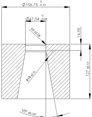
Experiments were performed for measuring drawing force for calibrating base FE model and verifying minimum possible thickness with various initial tube geometries. The machine for drawing tubes with variable thickness (Fig.6) was designed and fabricated completely by this group in the Laval University. Fig.s 7 and 8 show geometric details of die and mandrel and in Fig. 9 two different lubrication systems for the die and the mandrel are presented.
FIG.6) EXPERIMENTAL RIG FOR TESTS: 1) CYLINDER FOR PULLING THE TUBE, 2) LOCATION OF INSTALLATION OF DIE, 3) CYLINDER FOR MOVEMENT OF MANDREL [2].
FIG.6) GEOMETRIC DETAIL OF THE MANDREL USED IN EXPERIMENTS.
FIG.7) GEOMETRIC DETAIL OF THE DIE USED IN EXPERIMENTS
FIG. 8) THE LUBRICATION SYSTEMS FOR THE MANDREL (1) AND THE DIE (2). IN THE LUBRICATION SYSTEM 1 (FOR MANDREL) LUBRICATION REEL (3) WAS INSERTED FROM END OF TUBE AND MOVED WITH IT TO DELIVER LUBRICANT BETWEEN MANDREL AND TUBE. IN THE LUBRICATION SYSTEM 2 LUBRICANT WAS DISTRIBUTED BY LUBRICATION JETS. 2 2 3 5 1
3. RESULTS AND DISCUSSIONS
3.1. Validation of numerical results
For the first step, it was necessary to evaluate accuracy of the developed base FE model. In the table 2 the reaction forces on the die, mandrel and drawing forces are presented from FE and experiments. As mentioned before, the friction coefficients between die-tube and mandrel-tube were 0.067 and 0.132 respectively. The reason for assigning different friction coefficients for the die and mandrel was weakness of lubrication system for the mandrel in the designed machine. In this system the lubricant is injected by entering a reel from other end of tube and when there is small distance between tube and mandrel this reel can not deliver enough lubricant between mandrel and tube (Fig.8). The values which were presented in this table are for the initial tube thickness of 2.40mm and final thickness of 1.97mm with tube outer diameter of 53.98mm (2.125 inches). Based on the values presented in the table 2, it seems that the developed FE model has enough accuracy to be used in the optimization of process.
TABLE 2) VALIDATION OF BASE FE MODEL
3.2. Optimization results
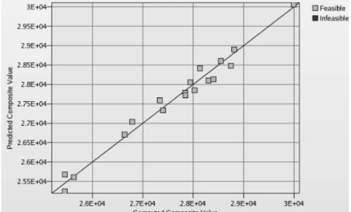
Fig. 9 presents model accuracy curve for a composite variable i.e. tube drawing force in the 5th iteration. This value is called composite because it is composed of two other variables i.e. reaction forces on the die and reaction forces on the mandrel. As it is clear in the Fig.9, all the points are feasible which means that they respected optimization constraint and there is acceptable difference among predicted and computed values. Predicted values were derived from the meta-model which represents the physical problem in each iteration and in some cases there will be some difference among these results and values obtained from simulation (computed values).
FIG. 9) METAMODELLING ACCURACY FOR COMPUTED FUNCTION (TUBE DRAWING FORCE).
Fig. 10 presents optimization history for the design variables i.e. initial thickness, outer diameter, and axial position of mandrel and corresponding final thickness in the best simulation of each iteration. As shown in these figures after 6 iterations (each iteration consisted of 28 simulations) the optimization has reached to a solution which respects the problem constraint and has maximum axial position of mandrel or in other words minimum tube thickness. As it is shown the final optimum geometry is 55.33 mm (OD) and 2.29 mm (th0) and the corresponding final thickness is 1.66 mm. In fact as it is shown in table 3, because of discrete dimensions of tubes while doing experiments it was not possible to do experiment with values obtained from the optimization but the experiments which were done in the upper and lower bound of obtained optimized points showed very good agreement between optimization results and average of experimental results.
TABLE 3) COMPARISON OF EXPERIMENTAL AND NUMERICAL OPTIMIZATION RESULTS
OD (mm) Th0 (mm) Final Thickness (mm) Experiment 1 53.98 2.40 1.65 Numerical Optimization 55.33 2.29 1.66 Experiment 2 63.49 2.40 1.93
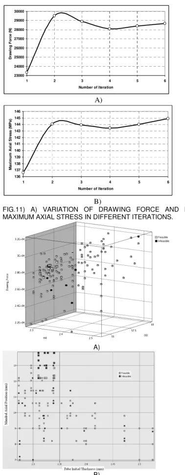
In Fig. 11, the history of drawing force and maximum axial stress were presented. As it is clear, in the iteration 2, despite having maximum drawing force and axial stress, the axial position of mandrel and correspondingly the final thickness of tube is not necessarily maximum which means that combination of these 3 parameters leads to optimum result.
2.28 2.29 2.3 2.31 2.32 2.33 2.34 2.35 2.36 2.37 2.38 2.39 2.4 2.41 1 2 3 4 5 6 Number of Iteration T u b e T h ic k n e s s ( m m ) A) 53.5 54 54.5 55 55.5 56 56.5 57 57.5 58 58.5 59 1 2 3 4 5 6 Number of Iteraton O u te r D im e te r (m m ) B) 7 8 9 10 11 12 13 14 1 2 3 4 5 6 Number of Iteration M a n d re l A x ia l D is p la c e m e n t (m m ) C) 1.5 1.6 1.7 1.8 1.9 2 2.1 2.2 1 2 3 4 5 6 Number of Iteration T u b e F in a l T h ic k n e s s ( m m ) D)
FIG. 10) OPTIMIZATION HISTORY FOR THE A) INITIAL THICKNESS (TH0) B) FOR THE TUBE OUTER DIAMETER (OD) C) MANDREL POSITION D) FINAL THICKNESS OF TUBE IN EACH ITERATION.
23000 24000 25000 26000 27000 28000 29000 30000 1 2 3 4 5 6 Number of Iteration D ra w in g F o rc e ( N ) A) 136 137 138 139 140 141 142 143 144 145 146 1 2 3 4 5 6 Number of Iteration M a x im u m A x ia l S tr e s s ( M P a ) B)
FIG.11) A) VARIATION OF DRAWING FORCE AND B) MAXIMUM AXIAL STRESS IN DIFFERENT ITERATIONS.
A)
C)
D)
FIG.12) SCATTER PLOT FOR SHOWING RESULT OF VARIOUS SIMULATIONS IN ALL ITERATIONS A) 3D SCATTER PLOT OF INITIAL THICKNESS (TH0) –OUTER DIAMETER (OD) VS. DRAWING FORCE B) 2D SCATTER PLOT OF TUBE INITIAL THICKNESS-MANDREL AXIAL POSITION C) 2D PLOT OF OUTER DIAMETER VS. MANDREL AXIAL POSITION D) 2D PLOT OF OUTER DIAMETER-TUBE INITIAL THICKNESS.
In Fig.12 scatter plots for showing results of all simulation points were presented. In Fig. 12A the dark points represent infeasible points which did not satisfy the optimization constraint. The interesting point about these infeasible points is possibility of having them in various combinations of OD and Th0 which confirms importance of appropriate selection of initial dimension of tube for this process. In Fig.12B, two dimensional scatter plot of tube initial thickness with respect to mandrel axial position which indirectly represents final thickness of tube was presented. As it was expected the points with more axial position (smaller final thickness) were more susceptible for passing the optimization constraint. Also with increasing the initial thickness the drawing situation got more difficult and some infeasible points were appeared in higher
values of initial thickness too. Almost the same explanation is valid for Fig.12C too. For the Fig.12D, number of infeasible points in smaller OD and smaller initial thickness are more than bigger levels of OD and Th0 which seems to be because of bigger values of axial position of mandrel (smaller final thickness) of tube.
4. CONCLUSION
The tube drawing process for production of variable thickness tubes was simulated by the Ls-Dyna software as a solver and optimized by the Ls-Opt software for evaluating effect of tube initial geometry (outer diameter and initial thickness) on the minimum possible final thickness. Based on the developed model, the maximum thickness reduction in the tube with various tube sizes were evaluated and optimum size was determined which was in good agreement with the performed experiments.
ACKNOWLEDGMENTS
The authors thank the National Sciences and Engineering Research Council of Canada, Alfiniti, Aluminerie Alouette, C.R.O.I and Cycles Devinci for the financial support of this research. A part of the research presented in this paper was financed by the Fonds québécois de la recherche sur la nature et les technologies by the intermediary of the Aluminium Research Centre – REGAL. Also technical supports from National Research Council, Aluminium Technology Centre and suggestions and helps of Mr. Jean-Francois Béland, researcher at this center were highly appreciated.
REFERENCES
1. Guillot M., Girard S., D’Amours G., Rahem A., Fafard M. 2010 "Experimental exploration of the aluminum tube drawing process for producing variable wall thickness components used in light structural applications", SAE 2010 World Congress, Detroit, USA.
2. Bratt J. F., Adami L., 1970 "On the Drawing Process of Thin- Walled Tubes of Anisotropic Material" Vol. 200, NO. 4, Journal of The Frankiiu Institute.
3. Pierlin I.L. and Jermanok M.Z. 1971, "Theory of Drawing", Mietallurgia, Moscow.
4. Collins I.F. and Williams B.K., 1985 "Slipline fields for axisymmetric tube drawing”, Int. J. Mech. Sci., 27 pp: 225-233.
5. Karnezis, P. E and Farrugia, D. C. J., 1998, "Study of cold tube drawing by finite element modeling", J. Mat. Proc. Tech. v. 80-81, pp:690-694.
6. Kim S.W., Kwon Y.N., Lee Y.S., Lee J.H., 2007 "Design of mandrel in tube drawing process for automotive steering input shaft" Journal of Materials Processing Technology (187) pp:182–186.
7. Kuboki T., Nishida K., Sakaki T., Murata M., 2008 "Effect of plug on levelling ofresidual stress in tube drawing", Journal of Materials Processing Technology, Volume204, Issues 1-3, 11, pp:162-168.
8. Bihamta R., D’Amours G., Rahem A., Guillot M., Fafard M., 2010 "Numerical studies on the production of variable thickness aluminium tubes for transportation purposes ", SAE2010 World Congress, Detroit, USA.
9. Hosford W. F., 2005. "Mechanical Behavior of Materials", Cambridge University Press.
10. Stander N., Roux W., Goel T., Eggleston T., Craig K. 2009 "LS-OPT User’s Manual" version 4.0.
11. Béland J.F., 2009 "Optimization of cold tube drawing of aluminium 6063-T4 with finite element method" M.Sc. thesis, Laval University, Quebec, Canada (In French).