Tax Mimicking and Sub-National Entities : Evidence at the Municipal Level for Montreal, 2000 ?

(1)

Rapport de Maîtrise

Tax mimicking and sub-national entities :

Evidence at the municipal level for Montréal, 2000?

Présenté par

Geneviève Gaboury

Gabg23527909

Université de Montréal

21 octobre 2004

(2)

Abstract

This paper tests if there is tax micmicking between municipalities for the urban area of

Montreal in 2000, two years previous to the merger of some of these municipalities

examined. The study uses a regression model (robust ordinary least squares) to estimate

the impact of demographic or economic variables on tax rates. The results show that

there is horizontal interaction between municipalities. An increase of 10% of the tax rate

of a neighbouring municipality leads to an increase of almost 4% in its own tax rate for a

municipality. Tax mimicking is the most plausible cause for the explanation of these

results since during the year 2000 there were no common shocks such as an

environmental catastrophe which would force the local governments to increase taxes.

Therefore, the local governments mimic the behaviour of their neighbours vis-à-vis the

tax rate.

(3)

List of table :

Table 1 :

Empirical Evidence on Tax Mobility/Reaction in Federal Countries,

1992-2002 p.8

Table 2 :

Empirical evidence on tax mimicking,1992-2002

p.25-26

Table 3 :

Summary of statistics p.31

Table 4 :

Estimates of model (by OLS robust) p.34

Table 5

:

Results of regression tax rate of previous years p.38

(6)

8

♦Introduction

The tax behaviour of sub-national entities (SNE) in a federation is an important aspect of

fiscal behaviour and probably the most important source of irritants, along with direct

subsidies to attract investments, in intra-country inter-SNE relations. We use sub-national

entity as a generic name for a province, state, county or municipality within a country

normally with a local government and a certain degree of autonomy in a varying number

of matters including taxation. Tax behaviour will be the focus of this paper; we will

leave aside subsidies, which are negative taxes and general SNE policies in fields such as

education, language or welfare that may have an impact on SNE economic attractiveness

and competitiveness. Tax behaviour has been the subject of both theoretical and, to a

lesser extent, empirical work by economists in the last twenty years or so. We will

examine in particular two tax behaviours; tax competition and tax mimicking. The first

one is observed when the entities try to enhance the attractiveness of their jurisdiction,

thus the entity decrease their taxes and the neighbouring entities must to do the same

thing, and this is the competition. Tax mimicking is the behaviour of entities which

imitate the tax behaviour of their neighbours, thus if an entity increase its tax rate theirs

neighbours will increase its own tax rate. Thus, in the first chapter, this paper will draw

on this existing body of work to examine three issues, each one corresponding to one part

of the paper. In the first part we present the main findings of the academic literature on

tax competition based on theoretical articles and empirical studies on actual behaviour

and by discussing the “ Tiebout hypothesis ”. In the second part, we provide the main

findings of the policy oriented literature towards what is proper SNE behaviour to adopt

(7)

to cope with harmful tax competition. The third part analyses the diverse view about tax

competition and what is good or bad about it. We present also why tax freedom is good

and we examine what are the consequences of tax competition and how this affects the

locational decisions of multinational firms. In the second chapter, we will present an

overview on the property taxation system in Quebec and also we will unveil some

empirical studies of tax mimicking behaviour and a theoretical analysis of our study. In

the third chapter, we will examine the results of an empirical study of the municipalities

of the Montreal Census Metropolitan Area (CMA) for the years 1998 to 2000 to ascertain

if there were tax competitiveness between the municipalities for the property tax rate of

2000 and what are the factors that influence this behaviour.

(8)

♦ Chapter 1 : Tax behaviour : tax competition *

1.1) The Academic Literature

There are two main streams of relevance to the tax behaviour of SNE. The first is the

academic one that is made up of theoretical articles, often making use of game theory,

that examine the possible behaviour of SNEs with respect to one another (and to the

central government) and of a limited number of empirical studies on actual behaviour.

Examining that literature on SNE tax behaviour, one is struck by the vocabulary used to

describe it. Perhaps the most common theme is tax competition. This is defined in The

Encyclopedia of Tax policy as «explicit or implicit». «Governments engage in explicit tax

competition when they enact tax laws and regulations expressly designed to enhance the

attractiveness of their jurisdictions to businesses, residents, employees or

consumers..(and) ..in implicit tax competition when they modify their pursuit of other tax

policy goals-such as equity, neutrality, simplicity, revenue adequacy, or tax exporting- in

order to mitigate anti-competitive consequences» (Tannenwald, 1999). Thus tax

competition is seen as something bad, which is odd given the connotation of good I

usually associated with competition in economics. In this case, good is associated with

tax harmonisation which does away with disharmony, something a priori difficult to

object to. Thereby, one slips from tax competition to tax disharmony with little regard for

what is meant exactly by harmonisation but with often the notion of uniformity

synonymous with harmony. For example, Cnossen and Shoup when discussing tax

(9)

harmonisation in Europe write that «EC policy makers appear to believe that members

states should first be forced in the strait-jacket of a uniform tax system»(emphasis ours;

Cnossen and Shoup, 1977, 82).

According to Wilson and Wildasin there are three definition of tax competition:

The broad definition : tax competition seems to be defined very broadly as any

form of noncooperative tax setting by independent governments.

The narrower definition : this definition adds the requirement that each

government’s tax policy influences the allocation of tax revenue across

government treasuries.

The narrowest definition : this define tax competition as noncooperative tax

setting by independent governments, under which each government’s policy

choices influence the allocation of a mobile tax base among “regions” represented

by these governments. In particular, governments may compete over the

allocation of workers, firms, capital, or shoppers.

Note that in empirical studies, authors often do not specify what definition is used.

There are diverse view in the theoretical literature on tax competition. Oates (1972)

describes this problem of tax competition as follows “ The result of tax competition may

(10)

attempt to keep taxes low to attract business investment, local officials may hold spending

below those levels for which marginal benefits equal marginal costs, particularly for

those programs that do not offer direct benefits to local business. ”

In fact, local officials will add to the conventional measures of marginal costs with those

costs such as reduced tax bases, lower wages and employment levels or capital losses on

homes or other assets that come up from the negative impact of taxation on business

investment. Those costs will reduce public spending and taxes to levels where the

marginal benefits equal the higher marginal costs. “ Oates’s conclusion that this

behaviour is inefficient rests on the idea that when all governments behave this way, none

gain a competitive advantage, and consequently communities are all worse off than they

would have been if local officials had simply used the conventional measures of marginal

costs in their decision rules.” (Wilson 1999)

“ Since the mid-1980’s, there has been an outpouring of academic research on tax

competition, and this research continues unabated. Interest in this area has been

stimulated by highly publicized instance where U.S. states and localities do seem to have

engaged in tax competition, including the many cases where they have offered large

subsidies to foreign and domestic automobile companies in an attempt to influence plant

location decisions. In addition, researchers and policymakers have found that Oate’s

(1972) description of tax competition can be applied more broadly to a host of important

policy concerns, such as competition for investment through weaker environmental

standards or reductions in welfare payments by states trying to avoid attracting poor

(11)

households.” (Wilson1999) There are diverse views about intergovernmental

competition but the main one is that competition is wasteful, that is induce lots of

questions about the role of the government and their appropriate behaviour and choices.

However, this is not the view of Tiebout. Indeed, Tiebout (1956) argues that

competition for mobile households is welfare enhancing and in the “Tiebout Hypothesis”

there is free factor mobility and enable national governments to function independently in

most policy areas.

In fact, the “Tiebout Hypothesis” is a theory of efficient tax competition and it leads to an

efficient provision of local public goods. “In modern formulations of the theory, it is

often assumed that each region’s government is controlled by its landowners, who seek to

maximize the after-tax value of the region’s land by attracting individuals to reside on

this land. To do so, the government offers public goods that are financed by local taxes.”

(Wilson1999) It indicates that there is tax competition since the region wants to attract

the persons or keep their residents providing the public goods at a low level of taxes.

The taxes are collected so that each resident pays a total amount equal to the cost of the

public goods consumed. With this marginal-cost-pricing rule each resident makes an

efficient decision about the choice of the region where they will live. Although these

results to apply to household mobility some authors such as Fischel (1975) and White

(1975) have extended them to mobile firm. They assume that firms are in infinitely

elastic supply to any given region. In equilibrium, the firms are taxed at a rate equal to

the cost of providing their “public inputs”, the marginal cost.

(12)

In fact, there are diverse views in the theoretical literature of tax competition and that is

the reason why most authors carry out empirical studies on actual behaviour. Studies

have been done on countries, districts, cantons and municipalities to measure tax

competition, its effect and consequences. One strand of literature reviewed by

Tannenwald is location studies. He notes that «hundreds of empirical studies have

investigated the extent to which a jurisdiction’s tax characteristics influence its

attractiveness. Most studies conclude that (1) taxes are a less powerful determinant of

business location and expansion than centrality of location, wage rates, regulatory burden

and the availability of appropriately skilled labour; and (2) ..taxes are a more effective

instrument of intrametropolitan competition than of intermetropolitan or interstate

competition.»(1999,p367); two points should be made here. First, location is one choice

and choice of jurisdiction were income, particularly capital income and corporate profits,

are reported is another. Second, distances in North America and in Europe are not the

same; what is inter state in North America may well be inter-country in Europe and intra

metropolitan, interstate.

A second strand of literature examines the impact of tax diversity either on tax related

choices of taxpayers or on the behaviour of governments (tax externalities). Five recent

studies(1993-) are summarised in the Table

1.

(13)

8

Table 1 : Empirical Evidence on Tax Mobility/Reaction in sub-national Countries, 1992-2002

Authors/year of study Country/Units/Years examined Number/Nature of observations

Methodology Used Main results Comments

Case, Rosen and Hines, 1993 U.S./ Continental United States/ 1970-1985 768 points data; 48states x 16years

First, a regression analysis is done by OLS with state public expenditures as DV and real per capita income, income squared, real per capita total federal grants to state and local governments, population density, proportion of the population at least 65 years old, proportion of the population between 5 and 17 years old, proportion of the population that is black as IV. After, they added three neighbor’s exogenous variable at the same regression; geographik proximity, per capita income and proportion black. Second, They estimated the model separately for four different types of expenditures: health and human services, administration, highways and education (equal to 75% of total expenditure). They used the same DV and IV but they used only the proportion black as neighbor’s exogenous variable.

The states’s expenditure are indeed significatly influenced by their neighbors. When we take in account neighbor effects substantially changes the estimed impacts of various conditionning variables on state expenditure. In addition, we note that spillovers need not be confined to subfederal jurisdictions but also to national governments.

The impact effect of a dollar of increased spending by a state’s neighbors increases its own spending by about 70 cents. Kirchgasnner et Pommerehne, 1996 Switzerland/Canton s/1987 156 cantonal-income groups share of taxpayers(26x7)

Regression analysis with share of taxpayers in group I as DV and PIT rate pre income group, % labour force in services, population, infrastructure index, and dummies for Zug and Geneva as IV

Tax rates play a significant role in determining where the highest income groups choose to locate particularly the highest. Infrastructure also plays a role

Income groups are 0-19(omitted),20-25,25-50,50-100,100-200 and >200 CHF

Regression is weighted with square root of population

Besley et Rosen, 1998

USA/48 continental states/1975-1989

720 state tax rates on tobacco and on gasoline =1440

Regression analysis with state tax rates as DV and IV: federal tax rate, national GDP and unemployment rate, state population, income and unemployment rate, %s population aged 5-17 and 65+, state production of tobacco and gasoline as %s state income,, federal grants per capita, federal income /AGI, Democrat governor, %s House and Senate democratic, Federal deficit/GDP, state effects

State tobacco tax increases by .028$ for a federal tax increase of .1$; for gasoline tax, the increase is .041$.

An increase in the size of the relevant industry decreases the tax rate in a given state.

Taking into account general sales taxes does not change the results. Vertical externalities are thus present

Hayashi et Boadway 2000 Canada/Federal, Ontario, Quebec and aggregate of remaining eight provinces 1961-1995 34 X4 =136 average effective tax rates(taxes paid/corporate profits)

Regression with each tax rate as DV; IV are the 3 other tax rates, national inflation and utilisation rate, provincial or Canadian GDP growth rate, interest rate, per capita wages, political party in power, deficit/GDP

Provincial tax rates of Quebec and 8 other provinces are diminished when the federal one is increased; an increase in the Ontario rate has a positive impact on the federal one; Ontario does not react to changes in provincial rates while Quebec reacts positively to an increase in the Ontario rate.

Seemingly Unrelated Regression system is estimated by GLS. Reaction lag is assumed to be one-period(one year)

The results show that vertical and horizontal externalities exist.

Mintz and Smart 2001 Canada/ aggregated corporate tax returns, 1986-1999 3509 data point ;14 years X6 regionsX7 industrial sectors X 6tax and size groupings(minus 19 missing data points)

Regression analysis with ln real taxable income per capita as DV and tax rate ,ln income prices , fixed effects and interactive province-industry variables as IV

Regressions are for three types of firms: (1)corporations that can shift taxable income easily versus those that cannot(2 and 3) results show a much higher tax elasticity for group (1) than (2) or (3)

The elasticity of 4.3 shows that a 1% point reduction in the mean tax rate(.43) increases taxable income by7.5%.No $ estimate of this impact is given;

DV: dependent variables; IV: independent variables Q for income quartile, (1 lowest, 5 highest

(14)

1.2) The Policy Literature

The second type of literature is more oriented towards policy, although it relies on some of the theoretical literature. It addresses the practical problems faced by countries that over the last 50 years have seen their borders become more and more open to flows of goods, services, capital and labour. It thus focuses on the behaviour of national governments (NGs) that are either the members of the European Union or members of the OECD ( Organisation for Economic Co-operation and Development) or interact as a tax haven with such a government. One should note here that until now, it has been common in the literature to draw lessons from federal states for the EU; yet, in some respects, the EU is a federal state, with a stronger central government than in true federal states. Thus, it may be time to ask what lessons the EU has for federal countries. In this case, one sees the emergence of the concepts of «harmful tax competition» defined below;

Harmful Tax Competition

No or Low Nominal Effective Tax Rate (generally or in special circumstances) +

One or more of:

• Lack of Effective Exchange of Information; • Lack of transparency;

• Ring fencing of domestic sector or attraction of investment without substantial activities Source: (Horner, 2000):

The key issue is the lack of information allowing the country of residence of the owner of an income stream the opportunity to levy the appropriate tax burden; this is embodied in

(15)

predatory tax practice. Reading on recent attempts (1997-2001) to harmonise taxation of income in the EU (Cattoir and Mors, 2001), one finds similar preoccupations.

We believe that the proper question is not “what is the appropriate degree of tax competition?” or “what is the required degree of tax harmonisation?” But rather; what are the appropriate tax choices of a given set of SNEs? This requires that criteria be set out and facts examined for each set of SNEs In particular, this means that we recognise that «since every country both is unique and in some sense constitutes an organic unity, the significance of any particular component of its federal finance system may be understood only in the context of the system as a whole» (Bird and Vaillancourt, 1998, p34-35).

Hence, what is proper SNE behaviour? The answer to this question will depend on each country. That said, one can note as Cattoir and Vaillancourt did (2002) that :

• One should distinguish between behaviour that influences real decisions, for instance the location or expansion of production units (manufacturing plants, call centers,..) and financial decisions, such as were to hold saving bonds and bank accounts. The first have meaningful economic consequences and revenue impacts while the second only have revenue consequences;

• Behaviour that influences financial decisions by individuals, for example, more or less strict banking secrecy laws and non communication of relevant tax information to the tax authority of the country of residence encourages tax avoidance and tax evasion. Clearly, all countries, federal or not, can suffer from the behaviour of third parties tax havens. Comparing the EU, a quasi-federal system to federations like Canada and the USA, one

(16)

notes that intra federal tax secrecy and tax residence issues matter more within the EU than within federal states. It is appropriate to combat this type of behaviour;

• Behaviour that influences real decisions is much less reprehensible. For example, if some SNEs have less mobile populations than others, for language reasons for example, they may want to lower the taxation of job creating investments to attract complementary capital to their (relative) excess labour. The other option, out-migration to where the capital is could well result in linguistic assimilation. This means ,in the absence of natural resource rents, that the residents of this SNE will have lower levels of public services or higher personal taxes ,or both;

• If an SNE has an exportable tax, such as natural resource rents, why should it not use it to make its residents better off? This will lower the tax price of a given supply of public services or increase the supply of such services. This will create disparities that a higher level of government can chose or not to correct in part or in total. That said, we would agree that natural resource rents should be collected by the central government which would do away with this issue;

• The fact that the behaviour of one SNE will influence that of other SNEs within a country or that of the central government, in terms of the setting of tax rates, is not a well-founded reason as such to prohibit such behaviour. The behaviour of one business unit often has impacts on that of others( prices, quantities), yet we leave it free to act.

(17)

1.3) Consequences and Importance of Tax Competition

Now, we can draw on this existing body of work to examine two issues. First, the tax competition can have bad or good aspects. Second, in spite of the consequences of competition there is evidence of the importance of this tax competition in countries.

First, some people maintain that tax competition is bad because it leads to lower tax rates on capital and public expenditure levels and reduces welfare. This is the view of Oates (1972), of Zodrow and Mieszkowski (1986) and Wilson (1986) (Wilson-Wildasin). Whereas, some people like Brennan and Buchanan (1980) (Wilson-Wildasin) believe that tax competition can be beneficial. Hence we now examine the bad and good aspects of tax competition.

1.3.1 ) Tax competition; why is it bad

There are various approaches to why tax competition is seen as bad. A first explanation is that, implicitly at least, the model of federalism used in the analysis is that of fiscal federalism and not of federal finance (Bird and Vaillancourt, 1998). In the fiscal federalism view of the world, one is decentralising responsibilities and revenues, with the norm being the centralised solution. Hence, one minimises distortion with respect to a centralised country with uniform taxation as very few countries make any significant use of regionally differentiated central income (personal or corporate) and consumption taxation as proposed by Buchanan (1950). In the federal finance view, one starts from a decentralised perspective where non uniformity is the norm and movement towards uniformisation are seen as having both costs and benefits that have to be traded –off against one another. In some sense, the issue is what is the default position for a federal country that is no longer federal; a centralised one or a set of new countries?

(18)

A second explanation draws on a combination of international economics and game theory. It defines good or bad not from a national perspective but from an international one. With such a perspective, well-conceived co-operation is usually preferable to non-co-operation. Tax competition will be seen as harmful if there are externalities associated with the tax policy choices of a national government considering when the policy choices are made. This leads to a larger definition of tax competition compared to the narrow legal one used by the EU and OECD.

One list of reasons why tax competition is bad is put forward by Tannenwald (1999,p370) and contains four elements:

• State and local tax incentives reward firms for behavior they would have exhibited any way;

• Tax competition ultimately lowers revenues without enhancing competitive standing and thus lowers spending for needed services;

• Tax incentives confer windfall in a capricious pattern, distorting the inter-industry allocation of resources;

(19)

Other authors associate three tax issues with fiscal competition. Boadway (2001) conveniently summarizes them as follows:

• Fiscal Inefficiency: this results from the fact that some regions have larger tax capacities than others, either on residence –based taxes (income,..) or on source –based taxes (natural resources,..) with the later capable of tax exportation and from the fact that some regions have larger needs (demography, topography,..) than others. In a unitary tax system, this is not apparent but emerges when there is decentralization. As a result, Net Fiscal Benefits( value of publicly provided goods ,services and transfers minus taxes paid) vary between regions ,creating an incentive to migrate and thus an inefficient allocation of resources between the regions of a given country;

• Horizontal Fiscal Externalities: this results from the fact that the tax choices of one region have an impact on another region. One distinguishes between positive and negative tax externalities. Positive externalities result from too low a tax rate in beggar thy neighbor type policies or too high a tax rate that reduces the tax base. Negative externalities result from tax exportation with a tax levied by one region being paid by the residents of another;

• Vertical Fiscal Externalities: this results from the interaction between the central level of government and SNEs. An increase in the tax rate of one level of government can have an effect on the tax revenues and /or tax rate(s) of the other level of government.

(20)

Also, the result that emerges from the framework developed by Wilson (1986) and Zodrow and Mieszkowski (1986) is that it lowers government spending and taxes below their efficient levels. Hoyt (1991), shows that in the Zodrow-Mieszkowski model (model of horizontal tax competition) the equilibrium capital tax, and welfare, falls as the number of regions rises. (Wilson-Wildasin 2001)

1.3.2) Tax competition; why is it bad and good

According to Musgrave (1997), tax competition can be good or bad depending on what type of competition one observes. The competition will be good for a jurisdiction if competition provides the right services at low cost and helps at designing efficient and equitable tax systems. In addition, decentralization with multiple jurisdictions supports this process at the local level. Whereas, if the jurisdiction offers low tax rates to attract capital and high income residents, in the long run the public services will be at an inefficient level and the use of capital will be less efficient. Indeed, Janeba (1998) combines competition over strategic trade policies with tax competition and conclude that tax competition leads to higher taxes or subsidies on mobile factors or firms. (Wilson and Wildasin )

(21)

1.3.3 ) Tax competition; why is it good

The first authors to express the hypothesis that the tax competition is good is Tiebout in 1956 as mentioned above. The “Tiebout hypothesis ” was that the households choose the jurisdictions according to their preferences about taxes and public expenditure. Therefore, competition among jurisdictions leads to an efficient local public good provision and consequently to an efficient tax competition.

The most provocative one is provided by Frey and Eichenberger (1996). They argue that the construct of a «social welfare maximising government . . . implicitly assuming democracy to work so well that no political distortions arise»(p339) is wrong. They note that the importance given to the approach reflects the small role played in the tax policy field by public choice theory. This theory argues that governments are not necessarily welfare maximising; politicians and/or bureaucrats that use them to their own benefits may capture the institutions of the state. This usually leads them to seek a greater level of government spending and thus a greater level of taxation. And since «harmonisation of taxes is an effective means to raise the tax level..»(p340), it is often a policy goal. The authors conclude by noting that:«societies face two kinds of distortions that reduce the welfare of individuals: economic distortions are induced by differential taxation and political distortions are induced by harmonized taxes. . . while the possibilities for reducing economic distortions have been extensively discussed in the literature, reducing political distortions has received less attention (347). Thus self-interest leads to the promotion of harmony/uniformisation.

(22)

Recently, most authors give attention to the possibility of tax competition can be beneficial. In fact, they argue that tax competition can lead to higher public expenditures and taxes on mobile factors and it could enhanced the efficience of tax competition.

Wilson (1999) points out that Brennan and Buchanan (1980) argue that tax competition improves welfare, because the size of government would be excessive in the absence of this competition.

More recently, Janeba et Schjelderup (nd) conclude that the political economy branch of the tax competition literature has a favorable outlook on tax competition which is seen as an instrument for curbing the rent seeking activities of government officials.

Thus, tax freedom can have good effects.

Tannenwald (1999,370) present a list of four items. They are:

• A reduction of the exploitation of taxpayers by leviathan;

• Encouragement to use the benefit principle which increases the efficiency of taxation; • Increased efficiency resulting from using the benefit principle;

• Encouragement of progressive taxation at the federal level where it is more appropriate

From a fiscal federalism perspective, the main argument to give SNEs freedom in setting their own taxes is that at the margin, one wants to make them accountable for their spending by requiring them to fund it from their own additional funds and not from transfer revenues.

(23)

Secondly, tax competition has many consequences. In fact, wasteful fiscal competition produce interregional externalities. Indeed, there is the fiscal externality that Boadway mentions. Another type of externality is the “pecuniary externality” that exists when regions are large enough to affect the product or factor prices confronting other regions and other externality could arise as a result of inefficiencies in private markets, coupled with the failure of governments to correct them.(Wilson 1999) In fact, when the governments doesn’t make the policy choice in the best interest of its residents, most of consequences can be emerge such as these externalities.

However, Wilson and Wildasin (2001) argue that “despite the ineffiencies associated with different tax rates, however, a tax harmonization policy without lump-sum transfers between regions will not necessarily make both regions better off, because it removes the ability of small regions to exploit large regions by undercutting their taxes” in the case of different regional size with different tax rates.

1.3.4 ) Tax competition and the locational decisions of multinational firms

Since 1980’s, numerous studies have been carried out to know what the effects of taxes are on economic development. The authors have attempted to determine whether taxes or other variables play a significant role in the decisions of the firms location. We can divide the different studies in two categories. The first one includes studies which examine the factors that influence the locational decisions of multinational firms. The second one includes studies which examine the same factors in cities, cantons, districts, state or provinces. We begin with two studies that have been done on multinational firms and their locational decisions.

(24)

In 1998, Devereux and Griffith examined the factors that influence locational decisions. They used a model in which firms produce differentiated products in imperfectly competitive markets and applied it to a panel of US firms locating in the European market. The results of the study is that agglomeration effects are important and the effective average tax rate influence the choice of location, but not the choice of whether to locate production in Europe compared with one of the outside options. The second study is Altshuler and Grubert (2001) examined how «the location decisions of US multinational corporations may change if the US were to adopt a system that exempts foreign dividends from home taxation.» (Altshuler and Grubert 2001) and provides no consistent or definitive evidence that location decisions would be significantly changed if dividends were to be exempt to be from US corporate tax.

As mentioned above, the second categories of studies examine the influence of a few factors on business location decisions for state, cities or cantons. In 1996, Robert Tannenwald wrote a paper in the New England Economic Review for the Federal Reserve Bank of Boston on « State business tax climate : How should it be measured and how important is it? ». In this paper, he investigated investments by manufacturing companies. He evaluated the business tax climates of 22 states in 1991 for five industries. Tannenwald analysed also if other factors than taxation such as wages, energy cost, the quality of public services and labour productivity can affect the location of business fixed investment. This study found a small effect that was statistically insignificant for the impact of state and local tax burden on business’s capital spending.

Since the last 30 years ago, many authors examined the impact of taxation on economic development. The results show small or no effect on locational decisions of firms. This is

(25)

maybe why in the last ten years few authors wrote on the subject. In fact, the majority of studies we done before 1990.

1.4 ) Conclusion

SNEs have varied degrees of freedom in setting their tax rates, defining their tax bases and administering their tax collection. This freedom is rated the highest amongst some of the richest and oldest federations of the world. While this observation should caution us against restricting it unduly, it must be coupled with the fact that in the case of Canada and the USA, physical distance may reduce the impact of such differences. Smaller distances in Europe, which do not appear to be compensated for by linguistic heterogeneity, make the issue more salient there.

While referring to the literature Janeba and Schelderup (nd), they conclude that;

“Early theory predicts that competition among regions over scarce capital will bid down taxes and expenditure to suboptimal levels. Later contributions have refined the analysis of tax competition to the extent that some models predict that taxes may actually increase as competition intensifies. The political economy branch of the tax competition literature has a favourable outlook on tax competition, which is seen as an instrument for curbing the rent seeking activities of government officials. Assuming that tax competition leads to inefficiently low taxes on capital and reduces welfare, tax coordination among a group of countries may improve welfare under certain conditions.”

(26)

♦ Chapter 2 : Taxation system in Quebec and analysis of studies of tax

mimicking

2.1) Taxation system for property taxes in Quebec *

In each province of Canada local government impose real property taxes and other property-based taxes; those taxes are the most important source of municipal revenue. (Finances of the nation 2002)

Property taxes are paid by the owners of real property, and on some measure of its value. The tax rate is expressed in dollars by 100$ of value (or 1000$ -the mill rate). For instance, the tax rate for Montreal is 1,99 in 2000, thus for each 100$ of taxable property, the taxpayers will paid 1,99$. These taxes are used to raise funds is local and regional municipal governments, school authorities and the provincial governments. (Finances of the nation 2002)

Real property is defined as the land and things permanently attached to the land. All provinces include land and building in their definitions of real property but some difference are present between provinces in the treatment of oil and gas wells, pipeline, mines, public-utility distribution systems and railways. (Finances of the nation 2002)

(27)

In Québec, real property is defined as «all immovables not explicitly excluded from the assessment rolls. It includes land, buildings, and machinery and equipment that service buildings ( for example, elevators and furnaces). Other taxable immovables include wharves, machinery foundations, tanks, chimneys, and handling systems. The definition excludes antipollution equipment, minerals, underground improvements at mine sites, railway property other than land and buildings, and immovables of natural gas, electricity, and telecommunication distribution systems that are subject to a special tax scheme in lieu of property taxes.» (Finances of the nation 2002, p 6:5).

«More recently, since January 1 in 2000, Québec municipalities are allowed to set five different tax rates for the following categories; industrial immovables, other non-residential immovables, immovables consisting of six or more dwellings, other residential immovables, and serviced vacant land.» (Finances of the nation 2002, p 6:12)

2.2) Former empirical study

We present empirical studies of the mimicking behaviour in Table 2 which summarizes the studies for the 1992- 2002 period. We resume seven studies but we mainly use four of them.

Ladd, in 1992, concluded that the burden of total taxes and the property tax burden increase if the neighbours’ taxes increased. Indeed, in 1978 when a neighbours tax increase of one dollar she reported an increase of 0.59$ for the burden of total taxes and 0.45$ for the property tax burden in their own tax rates and in 1985 we have increases of 0.82$ and 0.58$ respectively. Revelli (2001) concluded that a 10% increase in the local property tax rate of a district’s neighbours leads to an increase of 4-5% in its own property tax rate. Ladd’s study is different

(28)

from the other studies because it compares for 1978 and for 1985 the degree of clustering of tax burden among neighbouring counties within metropolitan areas to that among nonneighbouring counties within states with coefficient of variation. In fact, she examine if a county’s tax burden will have more impact on neighbouring counties within metropolitan areas than nonneighbouring counties within states.

(29)

Authors/ year of study Country/Units/ Years examined Number/Nature of observations

Methodology Used Main results Comments

Ladd, 1992 USA/ 248 large counties or county/ 1978 and 1985

496 points data ; 248 x 2 years

First, she did a comparison for 1978 and 1985 for the degree of clustering of tax burden among neighbouring counties within metropolitan areas to that among nonneighbouring counties within states with coefficient of variation. Secondly, the regression (with instrumental variables) are estimed separately for 1978 and 1985 data . The IV is local tax burden with DV : total taxes, property taxes, residential property taxes, general sales taxes, other taxes.

The local tax decisions in one jurisdiction are influenced by the tax burdens in neighbouring jurisdictions.

For example, in the regression, if the burden of total taxes on a county’s neighbors increase by 1$per 100$ of income, the burden in the county will increase by 0,59$ per 100$ in 1978 and the property tax burden by 0,45$. While in 1985 they increased by 0,82$ and 0,58$ respectively. Some of these differences may be explained by the nationwide “tax revolt”” of the late 1970’s and early 1980’s. Heydels and Vuchelen,1998 Belgium/municipal ities/1991 589 Local income tax (LIT)and local property tax (LPT)choices

3SLS estimations with either LIT or LPT as DV and IV: population, per capita income, % population <20 and also %>60, area and tax rates of neighbours.

In base equation, impact of Lit is increase in neighbour is .67% and in LPT .695%.. an increase in population increases tax rates while for income, it decreases them.

Additional analysis with income endogenous or different treatment of neighbours does not change results. Impact of neighbours diminishes with distance. Horizontal externalities are thus present Brett and Pinske ,2000 Canada-Province of British Columbia/municip alities/1987 and 1991 Business property taxes(BPT) for 147 municipalitiesX2= 294

Structural form and reduced form(with IV) analysis with BPT as DV and IV: median income ,own and neighbour; workforce in primary sector, own and neighbour; parks and roads per capita, distance from Vancouver, ,supra-municipal business tax rate and neighbours tax rate.

There is some evidence of neighbours tax rates and supra municipal tax rates affecting the choice of tax rates but it is not consistent from one estimation to another.

Adding fixed effects to the analysis reduces the number of significant coefficients

Revelli, 2001 UK/ English non-metropolitan districts/ 1983-1990 2368 points data ; 296 non-metropolitan districts x 8 years

Estimation procedure based on an instrumental variables approach (generalized method of moments) with local tax rate as DV and IV : the per capita rateable value, the Block Grant per capita, the proportion of domestic local tax rate base, the unemployment rate, a political controle variable (dummy variable) that equals one if the local council is controlled by the Labour Party and equals zero otherwise.

There is two different kinds of interaction. The results have conclued the presence of large and significant horizontal interaction between UK districts, but there is no evidence of positive correlation between district and county property tax

rates.Therefore, instead is compatible with tax mimicking at the local level.

A 10% increase in the local property tax rate of a district’s neighbours leads to an increase of 4-5% in its own property tax rate.

(30)

Brueckner and Saavedra, 2001

U.S./ cities from the Boston metropolitan area/ 1980 and 1990

140 points data ; 70 cities x 2 years

Regression analysis ( LM ) with property tax rates as DV and per capita income, per capita state aid, the African-American proportion of the

population, the proportion of the adult population with at least a college education, public sector earnings per capita, annual rate of population growth and population as IV. In addition, a IV equal to the city’s 1989 tax levy is added for the second regression (1990).

There is a empirical evidence on property-tax competition among local governments. In 1980 and 1990, there is strategic interaction in the choice of tax rates.

The strategic interaction still occurs in the post-Proposition 21/ 2

environment in the choice of business property taxes. The tax competition persisted despite the restrictions imposed by this tax limitation measure. Goodspeed, 2002 13 OECD countries,1975-1984,Aggregated local income tax revenues

130 country/year data points

Regression analysis (Tobit)with local income tax rate as DV and national income tax rate, local spending tax base mobility, and disparity, grants and fixed effects as IV

The higher the national tax rate, the lower the local one.

The higher the tax bases disparities and the higher Q1, the lower the rate.

Tax rate is revenue/GDP;

Disparity is Q5share/Q1share; Q1share as mobility.

Results indicate that vertical and horizontal externalities appear to occur

Revelli, 2002 UK/ English non-metropolitan district/ 1990 296 points data ; 296 non-metropolitan districts x 1 years

First, a Moran spatial statistic has been computed for the assessed levels of spending per capita, the actual levels of spending per capita and the property tax rates in 1990. Second, two regression by OLS with local public spending and local property tax rates as DV with IV; grant from central government, population size, a dummy for closeness to metropolitan areas to control for the presence of externalities form the (excluded) urban areas and a political control dummy to allow for systematic ideological differences. Third, a comparison between regression analysis by LM and IV approach with DV and IV.

The spatial autocorrelation is an important feature of local

governments’ expenditure decisions. The results support the hypothesis of spatially autocorrelated residuals in the local public expenditure determination equation and of mimicking behaviour in local property tax setting.

(31)

Secondly, the regression (with instrumental variables) are estimed separately for 1978 and 1985 data. It would be interesting if this study had used as an explanatory variable government subsidies in the regression because in other studies like Brueckner et Saavedra (2001), per capita state aid is significative.

Heydels and Vuchelen (1998) conclude that there is presence of horizontal externality for a study for Belgium in 1991. The results show that an increase of 10% of the tax rate of a neighbour will increase the tax rate of the jurisdiction by 6.95%. Moreover, the population of the municipalities and the proportion of the 60 year old people and more are two significant and positive variables and income is a significant and negative variable. In the study of Heydels and Vuchelen (1998) there is an important fact which is raised, it is that they find that the impact on the neighbours decreases with distance. In fact, they estimate coefficients for variables such as neighbours of first order and close to second order and the coefficient for those second-order is smaller. This is why, the impact is stronger for jurisdictions which share a border.

Brueckner and Saavedra (2001), study the cities of the urban area of Boston for 1980 and 1990 show that there is empirical evidence on property-tax competition among local governments. In 1980, the income per capita and the annual growth rate of the population have a negative impact on the rate of land tax and the per capita assistance given to the states per capita has a positive impact. In 1990, only the coefficients of the income per capita and the assistance given to the states have the same impacts. However, a new strongly significant and positive variable is the levy per capita (lagged). For the years 1980 and 1990, Brueckner and Saavedra observe a strategic interaction in the choice of the tax rates. This study uses a econometric model with spatial lags, estimates a reaction function of the representative

(32)

community, which connects the tax rates on the property of the community to its own characteristics and the tax rates of the communities in competition. (Brueckner and Saavedra 2001) The goal of their study is to see whether after the proposal 2 ½, which is a restraint measure of the tax imposed in 1981, there is still tax competition. The study was thus made for 1980 and 1990. However, the study shows that even after this proposal there is still strategic interaction in 1990. Yet, it would have been interesting to see whether with the passage of time between 82 and 90 this interaction would have decreased.

More recently, Revelli (2001) concluded that there is a large and significant horizontal interaction between UK districts (a entities used for administrative and other purposes) tax rates, but there is no evidence of positive correlation between district and county property tax rates. In fact, a 10% increase in the local property tax rate of a district’s neighbours leads to an increase of 4-5% in its own property tax rate. Moreover, his study reveals that the unemployment rate ( variable use as proxy for the local socio-economic conditions) and national grants have a negative impact on the local tax rate and the political variable (dummy variable) suggest that the authorities controlled by the Labour Party have higher tax rate than the authorities controlled by other parties (Conservative, Liberal Democrats). However, there is a weakness in the study because the unemployment rate variable is a proxy for income. In fact, there is no perfect correlation between income and unemployment rate, thus it would be necessary to have a corrected income between the differential of cost of living for districts to correct for this weakness.

Therefore, it is possible to note that some differences are present in these studies. Certain studies were carried out for one year and others for a longer period of time. Moreover, the authors do not use the same explanatory variables. Indeed, the variables which proved to be significant in certain cases were omitted in other studies. And the fact of taking variables

(33)

such as the rate of unemployment as proxy of the income (Revelli 2001) represents a weakness since there is no perfect correlation between these two variables.

However, we can see that in all these cases, there is a «mimicking ».

2.3) Theoretical analysis of our assumption

As noted above several authors have tried to analyse there interactions empirically. The majority of existing empirical studies indicate the presence of horizontal interaction between sub-national entities. These studies have been carried out for UK, United-States, Belgium and British–Columbia in Canada. We will examine if tax mimicking is indeed present in this province and in particular for the (CMA)of Montreal.

Hence we assume that the local government of a municipality which increases or decrease its property tax rate will incite the local governments of the closest municipalities to do the same creating strategic behaviour of the municipalities. With this approach, it will be thus possible to understand the dynamics of the choices of the local governments. And moreover, this study will make it possible to contribute to the general results.

The Montreal CMA was selected to test if there is tax competition since it is the largest urban area of Quebec and is composed of more than one hundred municipalities located continuously to one another. The list of all the municipalities as well as the values of the variables used for each one of them are found in appendix 1. Since some of the municipalities of Montreal were amalgamated in 2002, we will examine the tax behaviour of the municipalities for the year 2000 to avoid any behaviour in 2001 associated until the merger. Moreover, the study had to be done before the merger since after the merger we count only

(34)

28 municipalities. We will try to establish if the municipalities try to imitate the tax behaviour of their neighbour and if certain economic variables such as conditional subsidies for the year 2000 which are transfers of the provincial government granted to the municipalities, median household income, tax rate and demographic variables such as density of population and population influence the tax rate. We have summarized some statistics for our variables in the table 3 and there is also a small geographic map in appendix which represent all municipalities of the urban area of Montreal.

Table 3. Summary of statistics

Note: The data on the population, the density of population and the median income come from the census of 2001. The data on the tax rate and conditional subsidies come from http://www.mamsl.gouv.qc.ca/accueil.asp

The neighbour’s rate of 1999 is a variable which give an equal importance to the neighbours of each municipality. Hence, if a municipalities has three neighbours, each tax rate of this three municipalities will have a proportion of 1/3 in the calculation of the neighbour’s rate of 1999.

Variables Mean Median Standard Min. Max. Deviation

Tax rate 2000 (1$ per 100) 1,28 1,2545 0,332 0,493 2,296 Tax rate 1999 1,271 1,24 0,3414 0,493 2,301 Population 32630,70 13391 106335,98 893 1039534 Median household income ($) 54346,83 52337 14846,62 26317 95347 Density of population 1408,02 723,9 1601,40 13,6 7549,3 Conditional subsidies ($) 2034081,83 361988 12163741,4 0 122911500 Neighbour’s rate of 1999(Mi tit-1) 1,295 1,249 0,265 0,816 1,99

(35)

♦

Chapter 3 : Empirical Analysis

3.1 ) Model

We estimate the equation below to establish if there is horizontal interaction between municipalities of the urban area of Montreal. In this equation, index i refers to the municipalities (i = 1,…,105), index t refers to the financial year 2000 (t = 2000). The tax rate for the year 2000 is represented by tt, then we have variables such as population, median

income, density of population and conditional subsidies for the year 2000. In the equation, we have included the tax rate of the previous year as an explanatory variable. The error term is µ .

Tt = γ + α pop + β income + δ density.pop + τ Mi tit-1 + θ subsidies + µ

The parameter τ measure the horizontal interaction between the municipalities. The variable Mi is the ith row of the weight matrix M (105x105). To build this matrix a geographical

criterion was adopted. The element mij of the matrix will be equal to (1/number of

neighbourhoods of the municipality i ) if the municipality i and the municipality j share a common border and equal to zero otherwise. The sum of each row will be equal to one. This matrix is multiplied by the vector of tax rates with a one year lag thus tt-1 (1999). If we don’t

introduce this one year lag, we have a problem of endogeneity because tax rates of the municipality and its neighbours will be simultaneously determined. We have to carry out a White test to see if heteroscedasticity is present; there is heteroscedasticity. Therefore a regression using robust OLS will be carried out. By these estimates, we will find an horizontal interaction if the parameter τ is statistically significant.

(36)

3.2 ) Data and Results

In our equation, our dependent variable is the rate of tax for the year 2000 for the municipalities of the urban area of Montreal. As mentioned above, we have independent variables such as the resident population in each one of the cities and their population density, median income and conditional subsidies are included in our equation.

The regression will be for the 105 municipalities of the urban area of Montreal for the year 2000. Two municipalities of the 107 had to be excluded from our estimate. Dorval island and Cadieux island were omitted from our study because of their respective population and the median income for Cadieux island was not available. The results of our estimates of the regression by robust OLS are presented in table 4.

(37)

Table 4. Estimates of model (by OLS robust )

Variables OLS Neighbour’rate τ .391 * (.109) Population 1.91e-06* (9.24e-07)

Median Income -5.42e-07 (2.23e-06)

Population density .0000745 * (.00002)

Conditional subsidies 2000 -1.34e-08 (7.77e-09)

constant .660 * (.204)

Number of observations 105

R2 0.4897 Notes : The dependent variable is the property tax rate of 2000

The standard deviation are reported in parentheses * Significant at a level of 5%

(38)

The results of table 4 show that the median income of households and the conditional subsidies offered to local governments by the provincial government have a negative impact on the tax rates. However, these two variables are not statistically significant. Population has a positive impact on tax rates of 2000 with a estimated coefficient of 1.91e-06 and this variable is significant with a t-statistics of 2.073. Moreover, population density has a positive impact on the tax rates with a estimated coefficient of 0.0000745 but this variable is very significant with a t-statistic of 3.729. Therefore, a municipality which has a high density population and a large population will see its tax rate increase compared to another municipality which a lower density of population or population.

For the horizontal interaction, the results show that the interaction is very strong between municipalities. In fact, the estimated coefficient is very significant. The estimated coefficient is 0.391 with a t-statistics of 3.603. This result implies that an increase of 10% of the tax rate of a neighbouring municipality leads to an augmentation the tax rate of almost 4% in its own tax rate. Moreover, the R2of this regression is 0.4897, one can thus say that the model has appropriate explanatory variables.

The results reported that are similar to the results obtained in other empirical studies. For the United States, Ladd (1992) found correlation coefficient between counties’ tax burdens that range 0.45 to 0.82. Heydels and Vuchelen in 1998 found a coefficient for the tax rates in neighbouring municipalities of 0.695. Thus, an increase of 10% for a neighbouring municipality leads to an increase of 6.95% in tax rates for it is own municipality. Revelli in 2001, found for UK, that an increase of 10% in a local property tax rate of a district’s neighbour leads to an increase of 4-5% it is own property tax rate.

(39)

The results are compatible with two explanations. First of all, the relation which exist between a municipality and its neighbour municipality can be due to common shocks affecting the local government such as a shock on the expenditure of a municipality. Secondly, « tax competition among local jurisdictions and the existence of spill-over effects from local public expenditure might generate correlation in tax rates among neighbouring authorities.» (Revelli, 2001 p.1106). Thus, this second explanation implies that the tax mimicking is a explanation which one must retain.

Revelli (2001) concludes that horizontal interaction exists. He explains, why, this spatial auto-correlation observed between districts (a region marked off for administrative or other purposes) can be due to common shocks which affect only local government. For instance, «an environmental catastrophe (an event most likely to bring about neighbourhood effects) might force local authorities to levy higher taxes at the level of government that is responsible for environmental health (the district), but not at the upper level of government (the county)». (Revelli, 2001 p.1106) He concludes that the effect of tax mimicking cannot be excluded by suggesting that it would be the most plausible cause for the explanation of these results. He excluded with a reasonable degree from confidence the possibility that spatial dependence in property tax rates is simply due to the presence of common shocks.(Revelli, 2001p.1106)

In fact, the tax mimicking would be also the most probable cause for the explanation of our results. Indeed, for the years used in this study, no environmental catastrophe, no event which could have caused effects on the neighbour municipalities occurred in the urban area of Montreal. One can only reject assumption concerning the common shocks. It thus becomes obvious that the tax competition would be the most precise interpretation of our results.

(40)

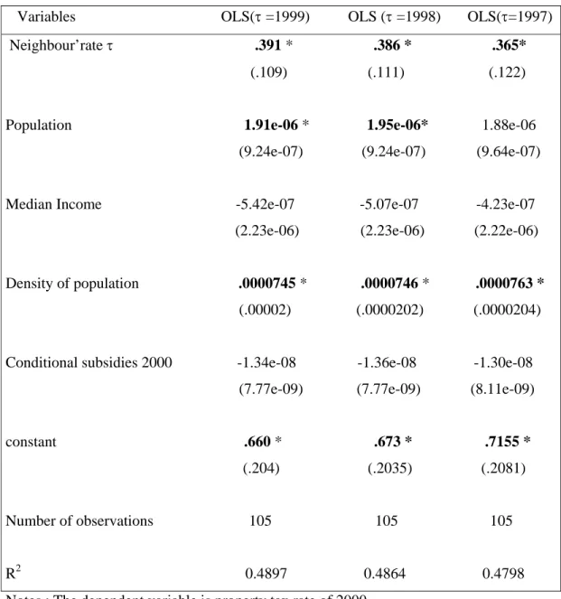
A interesting fact to accentuate is that the tax rate of previous years such as 1998, 1997 and so on, have also a impact but it decrease with the years. Moreover, the population become not significant in the last column. We can observe these results in table 5.

Table 5. Results of regression tax rate of previous years

Variables OLS(τ =1999) OLS (τ =1998) OLS(τ=1997) Neighbour’rate τ .391 * .386 * .365* (.109) (.111) (.122)

Population 1.91e-06 * 1.95e-06* 1.88e-06 (9.24e-07) (9.24e-07) (9.64e-07)

Median Income -5.42e-07 -5.07e-07 -4.23e-07 (2.23e-06) (2.23e-06) (2.22e-06)

Density of population .0000745 * .0000746 * .0000763 * (.00002) (.0000202) (.0000204)

Conditional subsidies 2000 -1.34e-08 -1.36e-08 -1.30e-08 (7.77e-09) (7.77e-09) (8.11e-09)

constant .660 * .673 * .7155 * (.204) (.2035) (.2081)

Number of observations 105 105 105

R2 0.4897 0.4864 0.4798 Notes : The dependent variable is property tax rate of 2000

The standard deviation are reported in parentheses * Significant at a level of 5%

(41)

♦ Conclusion

This paper used a regression model to examine if was tax competition presente between the municipalities of the Montreal CMA. The results obtained confirmed, the presence of horizontal interaction at the level of local governments. In fact, when a neighbouring municipality increase its tax rate of 10%, a municipality increase its own tax rate by almost 4%. Also, among the explanatory variables used only the density of population and the population are a significant and positive effect on tax rate. Moreover, the horizontal interaction is not due to common shocks that would affect the local government such as environmental catastrophe or a shock on the expenditure of a municipality in particular but rather by the behaviour of tax mimicking. In fact, the local government tend to mimic the behaviour of their neighbours for tax rate. These results support the assumption that there is a tax mimicking between the municipalities of the Montreal CMA.

(42)

Appendix 1

Table 6: municipalities and values of the variables used in the regression

Density of Conditional

Municipalities Tax rate of 98 Tax rate of 99 Tax rate of 2000 Population Median income

Population km 2 subsidies 2000 Anjou 1,48 1,55 1,55 38015 40828 2791,1 1018492 Baie-d'Urfé 0,9675 1,0419 1,0176 3813 90169 632,5 0 Beaconsfield 1,683 1,721 1,721 19310 88432 1754 575963 Beauharnois 1,63 1,63 1,63 6387 37207 156 634007 Bellefeuille 1,05 1,09 1,13 14066 51482 281,4 195921 Beloeil 1,454 1,4541 1,464 19053 50987 791 381796 Blainville 1,35 1,35 1,35 36029 62619 653,9 337440 Bois-des-Filion 1,0902 1,0902 1,0902 7712 50006 1803,2 582147 Boisbriand 1,095 1,131 1,134 26729 56157 962,8 816143 Boucherville 1,112 1,112 1,112 36253 71991 512,1 361923 Brossard 1,09 1,18 1,14 65026 55008 1421,6 1343414 Candiac 1,177 1,177 1,177 12675 69720 723,9 349581 Carignan 0,8937 0,8937 1,0014 5915 55202 94,8 934560 Chambly 1,2603 1,2797 1,3598 20342 52809 806,2 615764 Charlemagne 1,2872 1,3734 1,3734 5662 38706 2612,5 450931 Châteauguay 1,39 1,39 1,39 41003 50014 1142,4 1025043 Côte-Saint-Luc 1,633 1,677 1,677 30244 41028 4356 615334 Delson 1,21 1,21 1,25 7024 55205 985 165406 Deux-Montagnes 1,448 1,491 1,538 17080 53213 2773,7 1879476 Dollard-des-Ormeaux 1,74 1,9 1,86 48206 62590 3191,9 487087 Dorval 1,5472 1,5809 1,57 17706 48327 848,3 1000089 Gore 0,92 0,95 0,95 1260 30973 13,6 186221 Greenfield Park 1,4066 1,43 1,43 16978 44829 3555,1 409083 Hampstead 2,16 2,2652 2,2552 6974 89076 3895,9 278850 Hudson 0,7874 0,7874 0,9303 4796 58935 220,5 24207 Kirkland 1,5119 1,5119 1,5009 20434 87387 2119,5 220214 L'Assomption 1,1 1,1 1,1 15615 50224 157,9 226814 L'Île-Bizard 1,3871 1,3871 1,3177 13861 73098 608,7 280879 L'Île-Cadieux 0,5645 0,5829 0,5855 127 224 0 L'Île-Dorval 4,09 4,09 4,45 0 0 0 L'Île-Perrot 1,516 1,471 1,43 9375 47809 1686,9 1703364 La Plaine 1,5261 1,5261 1,5655 15673 47672 389,9 1000388 La Prairie 1,0329 1,0237 1,0184 18896 57272 432,5 619749 LaSalle 1,72 1,72 1,67 73983 39655 4417,5 1861081 Lachenaie 1,1544 1,1944 1,1944 21709 62218 516 704267 Lachine 1,43 1,48 1,45 40222 35126 2256 1462983 Lafontaine 0,99 1,04 1,1 9477 40247 659,8 14588 Laval 1,609 1,697 1,6714 343005 49194 1388,3 24276391 Lavaltrie 1,125 1,125 1,127 5967 46853 2123,9 310024 Le Gardeur 1,3693 1,39 1,33 17668 57486 473,9 361988 LeMoyne 1,465 1,465 1,465 4855 30604 4852,6 10210 Les Cèdres 0,8815 0,8965 0,9659 5128 58091 65,4 120003 Longueuil 1,627 1,655 1,683 128016 38344 2909,2 6695279 Lorraine 1,0558 1,0558 1,0774 9476 86889 1568,6 203674

(43)

Density of Conditional

Municipalities Tax rate of 98 Tax rate of 99 Tax rate of 2000 Population Median income Population km2

Subsidies 2000 Léry 0,493 0,493 0,493 2378 51051 224,9 5168 Maple Grove 0,69 0,69 0,69 2628 45538 309,6 34497 Mascouche 1,4147 1,4196 1,4079 29556 53499 277,2 464363 McMasterville 1,145 1,185 1,185 3984 50390 1284,6 82263 Melocheville 1,0614 1,0614 1,0614 2449 45224 129,6 114567 Mercier 1,0403 1,0486 1,0722 9442 55972 205,5 545704 Mirabel 0,94 0,94 0,94 27330 49061 56,3 577830 Mont-Royal 1,29 1,29 1,29 18682 75473 2438,3 264320 Mont-Saint-Hilaire 0,95 1 1 14270 62153 322,2 860203 Montréal 1,99 1,99 1,99 1039534 31771 5590,8 122911500 Montréal-Est 1,53 1,56 1,56 3547 38142 284,8 656943 Montréal-Nord 1,75 1,72 1,72 83600 27529 7549,3 401562 Montréal-Ouest 2,2553 2,3012 2,2956 5172 88209 3675,4 0 Notre-Dame-de-l'Île-Perrot 0,9092 0,9267 0,9267 8546 71383 307,5 157362 Oka 1,23 1,28 0,97 3194 51809 53 230454 Otterburn Park 1,215 1,265 1,315 7866 56499 1470,9 576023 Outremont 1,375 1,54 1,54 22933 61979 5984,3 1949106 Pierrefonds 2,12 2,12 1,965 54963 52337 2207,2 423940 Pincourt 1,5738 1,6246 1,5828 10107 60546 1340 114157 Pointe-Calumet 1,09 1,09 1,09 5604 39710 1211,2 23995 Pointe-Claire 1,447 1,4679 1,4679 29286 61133 1552,2 601650 Pointe-des-Cascades 1,15 1,15 1,15 913 58224 327,6 181633 Repentigny 1,21 1,21 1,21 54550 58110 2228 1603410 Richelieu 1,075 1,075 1,075 4851 45142 156,3 87581 Rosemère 0,81 0,88 0,825 13391 74708 1243 618314 Roxboro 1,8718 1,84 1,812 5642 58881 2544,4 157086 Saint-Amable 1,0954 1,2213 1,4025 7278 44365 198,4 348808 Saint-Antoine 1,48 1,47 1,45 11488 42358 1156,9 137753 Saint-Antoine-de-Lavaltrie 0,9916 0,9615 0,9914 5196 47288 79,5 10980 Saint-Basile-le-Grand 1,179 1,179 1,179 12385 62390 343,1 326846 Saint-Bruno-de-Montarville 0,8575 0,8675 0,8775 23843 69290 551 1573568 Saint-Colomban 1,0698 1,1331 1,1309 7520 48097 80,4 577830 Saint-Constant 1,128 1,206 1,2416 22577 60031 394 428015 Saint-Eustache 1,422 1,407 1,35 40378 49913 581,6 1452800 Saint-Hubert 1,438 1,435 1,444 75912 51810 1150,6 1131649 Saint-Isidore 0,79 0,79 0,79 2371 47153 45,6 49490 Saint-Joseph-du-Lac 1,2252 1,205 1,2545 4882 58059 118 8628 Saint-Jérôme 1,45 1,57 1,64 24583 26317 1514,8 1474232 Saint-Lambert 1,29 1,29 1,29 21051 53928 2584 1354020 Saint-Laurent 1,38 1,38 1,38 77391 39412 1804,7 2331927 Saint-Lazare 0,674 0,674 0,708 12895 76091 193,8 1644709 Saint-Léonard 1,7569 1,7569 1,7569 69604 38328 5149 884100 Saint-Mathias-sur-Richelieu 0,9181 0,918 0,9181 4149 53568 87,9 267903 Saint-Mathieu 0,862 0,862 0,862 1961 45253 62,1 10492 Saint-Mathieu-de-Beloeil 0,766 0,766 0,7743 2236 68709 56,1 219717 Saint-Philippe 0,9382 0,94 0,9391 3892 48544 62,6 134543 Saint-Placide 1,0391 1,0408 1,04 1537 29691 35,6 116359

(44)

Density Conditional

Municipalities Tax rate of 98 Tax rate of 99 Tax rate of 2000 Population Median income Population km2

Subsidies 2000 Saint-Sulpice 0,28 0,54 0,6007 3343 54821 91,9 6175 Sainte-Anne-de-Bellevue 1,2622 1,3002 1,2999 5062 44092 479 161161 Sainte-Anne-des-Plaines 1,24 1,24 1,295 12908 47271 139,1 225586 Sainte-Catherine 1,0738 1,0542 1,0821 15953 55103 1565,6 143729 Sainte-Geneviève 1,585 1,625 1,625 3278 34427 3816,1 12400 Sainte-Julie 1,047 1,05 1,059 26580 69082 536,7 760696 Sainte-Marthe-sur-le-Lac 1,387 1,387 1,5026 8742 47816 938,6 216207 Sainte-Thérèse 1,19 1,29 1,3 24269 40388 2533,9 1210648 Senneville 1,0138 1,0818 1,081 970 95347 129,6 1190 Terrasse-Vaudreuil 1,2739 1,2616 1,2432 2047 54121 1977,2 5823 Terrebonne 1,1254 1,3276 1,3276 43149 48723 598 1068492 Varennes 0,662 0,766 0,746 19653 66703 212,4 273549 Vaudreuil-Dorion 1,03 1,05 1,155 19920 54728 274,9 4416476 Vaudreuil-sur-le-Lac 0,8606 0,8814 0,8815 893 81258 650,5 9720 Verdun 1,52 1,5201 1,54 60564 35176 6166 1957958 Westmount 1,35 1,35 1,35 19727 78611 4902,8 240008

Tax Mimicking and Sub-National Entities : Evidence at the Municipal Level for Montreal, 2000 ?

Rapport de Maîtrise