Non-quadratic anisotropic potentials based on linear transformation of plastic strain rate

Science Arts & Métiers (SAM)

is an open access repository that collects the work of Arts et Métiers Institute of Technology researchers and makes it freely available over the web where possible.

This is an author-deposited version published in: https://sam.ensam.eu

Handle ID: .http://hdl.handle.net/10985/9911

To cite this version :

Daeyong KIM, Frédéric BARLAT, Salima BOUVIER, Meziane RABAHALLAH, Tudor BALAN, Kwansoo CHUNG - Non-quadratic anisotropic potentials based on linear transformation of plastic strain rate - International Journal of Plasticity - Vol. 23, n°8, p.1380–1399 - 2007

NON-QUADRATIC ANISOTROPIC POTENTIALS BASED ON

LINEAR TRANSFORMATION OF PLASTIC STRAIN RATE

Daeyong Kim 1, Frédéric Barlat 2, Salima Bouvier 3, Meziane Rabahallah 4, Tudor Balan 4, Kwansoo Chung 5,§

1

Materials Research Team, Corporate R&D Division for Hyundai Motor Company & Kia Motors Corporation, 772-1, Jangduk-dong, Hwaseong-si, Gyeonggi-do, 445-706,

Korea

2

Alloy Technology and Materials Research Division, Alcoa Technical Center, 100 Technical Drive, Alcoa Center, PA 15069-0001, U.S.A.

3

LPMTM-CNRS, UPR9001, University Paris13, 99 Av. J.-B. Clément, 93430, Villetaneuse, France

4

LPMM-CNRS, UMR7554, ENSAM de Metz, 4 rue A. Fresnel, 57078, Metz cedex 3, France

5

Department of Materials Science and Engineering, Intelligent Textile System Research Center, Seoul National University, 56-1, Shillim-dong, Kwanak-gu, Seoul, 151-742,

Korea December 11, 2006

ABSTRACT

In this paper, anisotropic strain rate potentials based on linear transformations of the plastic strain rate tensor were reviewed in general terms. This type of constitutive models is suitable for application in forming simulations, particularly for finite element analysis and design codes based on rigid plasticity. Convex formulations were proposed to describe the anisotropic behavior of materials for a full 3-D plastic strain rate state (5 independent components for incompressible plasticity). The 4th order tensors containing the plastic anisotropy coefficients for orthotropic symmetry were specified. The method recommended for the determination of the coefficients using experimental mechanical data for sheet materials was discussed. The formulations were shown to be suitable for the constitutive modeling of FCC and BCC cubic materials. Moreover, these proposed strain rate potentials, called Srp2004-18p and Srp2006-18p, led to a description of plastic anisotropy, which was similar to that provided by a generalized stress potential proposed recently, Yld2004-18p. This suggests that these strain rate potentials are pseudo-conjugate of Yld2004-18.

§

Corresponding author. Tel.: +82-2-880-7189; Fax: +82-2-885-1748 E-mail address: kchung@snu.ac.kr (K. Chung).

KEYWORDS: Constitutive model, Plastic anisotropy, Sheet material, Strain rate

potential

1. INTRODUCTION

In order to represent the rate-insensitive plastic behavior of materials phenomenologically, it is typical to use a yield function (for a yield surface), the associated flow (or normality) rule and a hardening law. The first two express anisotropic relationships between the stress and plastic strain rate components at a given material point (in terms of a parameter representing the accumulated plastic strain). The yield function φ gives the stress at which yielding occurs for a given stress state, and its gradient (the normal to the yield surface at the loading point) gives the direction of the plastic strain rate εɺ ; i.e.,

φ λ∂ = ∂ ε s ɺ ɺ (1)

where s is the stress deviator and λɺ is a proportionality factor necessary to scale the strain rate. The hardening law expresses the evolution of the yield surface.

Ziegler (1977) and Hill (1987) have shown that, based on the plastic work equivalence principle, a meaningful strain rate potential can be associated with any convex stress potential (or yield surface). Therefore, an alternative approach to describe plastic anisotropy is to provide a strain rate potential ψ, which is expressed as a function of the traceless plastic strain rate tensor εɺ , while its gradient leads to the direction of the stress deviator s; i.e.,

ψ µ ∂ = ∂ s ε_ɺ (2)

In Eq. (2), µ is a proportionality factor necessary to scale the stress deviator (and its value is related to the reference stress such as the uniaxial stress in a particular direction, according to the plastic work equivalence principle). This approach based on the strain rate potential was applied for FCC single crystals (Fortunier, 1989) and BCC

based on crystallographic texture functions were also used in finite element simulations of forming processes (Bacroix and Gilormini, 1995; Szabó and Jonas, 1995; Hu et al., 1998, Zhou et al., 1998; Li et al., 2001).

While the development of stress potentials has been diverse, that of strain rate potentials has been rather inactive with little interest. One reason is that their analytical expressions are very difficult or impossible to obtain as conjugate (dual) quantities of stress potentials, utilizing the equivalence of plastic work rate. A few simple descriptions such as Mises, Tresca, Hill’s old (1948) and a special case of Hill’s new (Hill, 1979) potentials are exceptions. Nevertheless, in an effort to develop the phenomenological description of plastic behavior for textured polycrystals, Barlat and his colleagues have proposed a series of stress and strain rate potentials suitable to characterize plastic anisotropy for plane stress and full (3-D) stress states. None of these stress and strain rate potentials are strictly conjugate (dual) of each other but it was observed that some pairs are pseudo-conjugate** because they lead to very similar plastic behavior. The stress-based potentials are useful especially for elasto-plastic formulations, while the strain rate potentials are convenient to use for rigid-plastic formulations (the effort to numerically derive strain rate potentials from stress potentials for rigid-plastic formulations can be found in the work by Zhou and Wagoner (1994)). Barlat et al. (1991) developed the stress potential Yld91 for general stress states, which was applied for elasto-plastic finite element analysis by Chung and Shah (1992) and Yoon et al. (1999a; 1999b). Later, the strain rate potential Srp93 (Barlat and Chung, 1993; Barlat et al., 1993), which is the pseudo-conjugate of Yld91, was developed for application to process design (Barlat et al., 1994; Chung et al., 1997) as well as process analysis (Chung et al., 1996; Lee et al., 1997; Yoon et al., 1995; Ryou et al., 2005), based on rigid-plastic formulations. In its application, the ideal forming theory (Chung and Richmond, 1992a; Chung and Richmond, 1992b; Chung and Richmond, 1994; Chung et al., 2000) was utilized for process design based on the deformation theory (Chung and Richmond, 1993) under the one-step backward formulation, while the incremental deformation theory was utilized for process analysis based on minimum plastic work paths under the updated Lagrangian forward multi-step formulation. The potentials Yld91 (stress) and Srp93 (strain rate) are valid for orthotropic anisotropy and, for sheet forming applications, they use either uniaxial flow stresses or r values (width-to-thickness plastic strain rate ratios in uniaxial tension) for the identification of anisotropy coefficients. In order to use both flow stresses and r values simultaneously, the stress potential Yld96 (Barlat et al., 1997) and the strain rate potential Srp98 (Chung

**

The terminology is rather loose here since there is no rigorous mathematical

relationship between the pairs except the commonalities in the non-quadratic nature and the number of anisotropic coefficients.

et al., 1999) were developed. The stress potential Yld96 was applied for the analysis of earing profile in the cylindrical cup drawing of 2008-T4 (Yoon et al. 1998) and 2090-T3 (Yoon et al. 2000) aluminum alloy sheet samples. For processes design, the potential Srp98 was applied to the optimization of a convoluted initial blank shape for the purpose of reducing the earing percentage in cup drawing (Yoon et al., 1999), and also for the optimization of the hydroforming process (Yoon et al., 2002; Chung, 2004). These potentials, Yld96 and Srp98, were shown to improve the accuracy of predictions compared to Yld91 and Srp93.

Although Yld96 and Srp98 were able to describe the plastic behavior of sheet metals accurately, their convexity was not rigorously proven. Moreover, their mathematical forms were not convenient for implementation into finite element codes. Therefore, the stress potential Yld2000-2d was proposed (Barlat et al., 2000, 2003) for the plane stress condition with rigorous proof of convexity. The stress potential Yld2000-2d is based on two linear transformations of the stress deviator and contains 8 anisotropy coefficients. Therefore, it can account for the flow stresses (

σ

₀,

σ

₄₅,

σ

₉₀) and r values (r₀, r₄₅,

90

r ) in uniaxial tension (where 0, 45 and 90 correspond to uniaxial tension along rolling, 45° from rolling and transverse directions, respectively) as well as the flow stress (

σ

_b) and strain rate ratio (rb = ɺεyy εɺ ) in balanced biaxial stress tension (where x and y refer xx

to the rolling and transverse directions, respectively). Yld2000-2d is similar to Yld96 in its capability to describe anisotropy but it is more convenient to use for finite element applications. This potential was used for springback analysis (Chung et al., 2005; Lee et al., 2005a; Lee et al., 2005b) and forming limit calculation (Kim et al., 2003a) for automotive sheet samples as well as for the forming analysis of aluminum alloy sheets (Yoon et al., 2004). The strain rate potential Srp2003-2d, which is the pseudo-conjugate of Yld2000-2d, was proposed by Kim et al. (2003b) subsequently.

The formulation based on two linear transformations of the stress deviator Yld2000-2d was extended to the general (3-D) stress state with the stress potential Yld2004-18p (Barlat et al., 2005). Because Yld2004-18p contains 18 anisotropy coefficients, it can account for the flow stresses and r values in tension at every 15 degrees from the rolling direction for sheet forming applications. As a result, Yld2004-18p can lead to the predictions of six or eight ears in finite element simulations of the cup drawing process, as observed for some aluminum alloy sheets (Yoon et al., 2006).

is minimized in order to determine the anisotropy coefficients, is discussed in Section 4. Applications of these strain rate potentials to the modeling of plastic anisotropy for aluminum alloy and dual phase steel sheet samples are presented in Section 5.

2. STRAIN-RATE POTENTIALS: SRP2004-18P AND SRP2006-18P

The full 3-D anisotropic plastic strain rate potential ψ , denoted Srp2004-18p (Barlat and Chung, 2005), was formulated based on the following column matrix with six arguments E= E Eɶ₁′ ′, ɶ₂, E E E Eɶ₃′, ɶ₁′′ ′′ ′′, ɶ₂, ɶ_3T; i.e., 1 2 3 2 2 3 3 1 1 2 ( ) ( , ) ( , ) (2 2) b b b i j b b b _{b b} E E E E E E E E E E E ψ ψ ψ ψ ε − ′ ′′ ′ ′′ ′ ′ ′ = = = = + + ′′ ′′ ′′ ′′ ′′ ′′ + + + + + + = + E E Eɶ ɶ ɶ ɶ ɶ ɶ ɶ ɶ ɶ ɶ ɶ ɶ ɶ ɺ (3)

Alternatively, a similar potential called Srp2006-18p is introduced in this work as

1 2 3 1 2 3 2 ( ) ( , ) ( , ) (2 2) b b b b b b i j b b E E E E E E E E

ψ ψ

ψ

ψ

ε

− ′ ′′ ′ ′′ ′ ′ ′ ′′ ′′ ′′ = = = = + + + + + = + E E Eɶ ɶ ɶ ɶ ɶ ɶ ɶ ɶ ɶ ɶ ɺ (4)

All the equations of this section are equally applicable to both potentials. Here, εɺ is the effective plastic strain rate, which is the conjugate of the effective stress σ under the plastic work rate equivalence principle:

σ ε

ɺ =s_ij

ε

ɺ_ij for isotropic hardening††. Also,

i

E′ɶ and E′′ɶ are the principal values of tensors ′_i εɶɺ and ′′εɶɺ , which are defined by two

linear transformations on the traceless plastic strain rate tensor eɺ for incompressible plasticity ′= ′ = ′ ′′= ′′ = ′′ ε _{B e B Tε} ε _{B e B Tε} ɶ _ɺ ɺ ɺ ɶ _ɺ ɺ ɺ (5)

In Eq. (5), both B and ′ B contain anisotropic coefficients as represented by ′′

††

The proposed plastic strain rate potentials (and its effective plastic strain rates) are also valid for the isotropic-kinematic hardening model, based on the modified and general plastic work equivalence principle (Chung et al., 2005).

12 13 21 23 31 32 44 55 66 0 0 0 0 0 0 0 0 0 0 0 0 0 0 0 0 0 0 0 0 0 0 0 0 0 0 0 b b b b b b b b b − −     − −   _{− −}  =             B (6)

for orthotropic symmetry. In Eq. (5), eɺ=Tεɺ is another expression of the traceless plastic strain rate tensor, necessary to ensure that the strain rate potential is a cylinder through the transformation represented by T

2 1 1 0 0 0 1 2 1 0 0 0 1 1 2 0 0 0 1 0 0 0 3 0 0 3 0 0 0 0 3 0 0 0 0 0 0 3 − −     − −   _{− −}  =           T (7)

The ε_{ɺ -like tensors are written here as 6-component vectors; e.g.,}

T xy zx yz zz yy xx ] [

ε

_ɺ

ε

_ɺ

ε

_ɺ

ε

_ɺ

ε

_ɺ

ε

_ɺ ɺ =

ε _{, with components in the frame of material}

symmetry.

Note that the potentials are isotropic when the 18 anisotropic coefficients become identical, typically one. Even though two potentials defined in Eqs. (3) and (4) look similar, they differ each other except for isotropic cases so that one may perform better depending on sample materials. Also, note that

3 1 0 ii i ψ ε = ∂ ∂ =

∑

ɺ so that Eq. (2) is valid for these potentials. The value of the exponent b in Eqs. (3) and (4) is associated with the crystal structure. On the basis of micromechanical computations, 3 / 2 and 4 / 3 are recommended for BCC and FCC cases, respectively (Barlat and Chung, 1993), although this parameter can also be optimized in the set of material parameters during the identification process. Also, note that the strain rate potentials are scaled in Eqs. (3) and (4) considering that the reference state is uniaxial tension.

xx xy zx xy yy yz zx yz zz

ε

ε

ε

ε

ε

ε

ε

ε

ε

    =       ε ɶ ɶ ɶ ɺ ɺ ɺ ɶ ɶ ɶ ɶ _{ɺ ɺ ɺ} ɺ ɶ ɶ ɶ ɺ ɺ ɺ (8)

and its principal values are the roots of the characteristics equation,

3 2

1 2 3

( _k) _k 3 _k 3 _k 2 0

P Eɶ = −Eɶ + H Eɶ + H Eɶ + H = (9)

where H1, H2 and H3 stand for the associated 1st, 2nd and 3rd principal invariants of εɶɺ

(

)

(

)

(

)

1 2 2 2 2 2 2 2 3 (a) 3 (b) 3 (c) 2 2 xx yy zz yz zx xy yy zz zz xx xx yy yz zx xy xx yy zz xx yz yy zx zz xy H H H

ε

ε

ε

ε

ε

ε

ε ε

ε ε

ε ε

ε ε ε

ε ε ε

ε ε

ε ε

ε ε

= + + = + + − − − = + − − − ɶ ɶ ɶ ɺ ɺ ɺ ɶ ɶ ɶ ɶ ɶ ɶ ɶ ɶ ɶ ɺ ɺ ɺ ɺ ɺ ɺ ɺ ɺ ɺ ɶ ɶ ɶ ɶ ɶ ɶ ɶ ɶ ɶ ɶ ɶ ɶ ɺ ɺ ɺ ɺ ɺ ɺ ɺ ɺ ɺ ɺ ɺ ɺ (10)

Using the change of variables,

1

k k

Eɶ =E +H (11)

the characteristic equation, Eq. (9), becomes

3 ( _k) ( _k) _k 3 _k 2 0 P Eɶ =P E = −E + pE + q= (12) where

(

)

(

)

2 1 2 3 1 1 2 3 3 2 (a) 0 (b) 2 3 2 2 (c) arccos p H H q H H H H q p

θ

= + > = + +   = _{ }   (13)

The sign of p is obtained by the direct combination of the relationships in Eqs. (10)a and (10)b. Now, Cardan’s solutions of Eq. (12) are

1 3 1 3 1 1 3 1 3 2 1 3 1 3 3 (a) (b) (c) E z z E z z E z z

ω

ω

ω

ω

= + = + = + (14)

In Eq. (14), the complex number z is defined as

3 2

z= +q i p −q (15)

with the principal argument θ such that 0≤ ≤ and θ π 3 2

0

− ≥

p q , while

ω

is a complex constant (e−2iπ3), and z and

ω

are the respective conjugate quantities of z and ω.

The principal values of εɶɺ , which are real since p3−q2 ≥0, are

2 1 1 1 1 2 1 2 2 2 1 1 2 1 2 3 3 1 1 2 1 (a) 2 cos 3 4 (b) 2 cos 3 2 (c) 2 cos 3 E E H H H H E E H H H H E E H H H H

θ

θ

π

θ

π

  = + = +  +   +   = + = +  +   +   = + = +  +   ɶ ɶ ɶ (16)

These values are ordered

1 2 3 or 1 2 3

E >E ≥E Eɶ ≥Eɶ >Eɶ (17)

as shown in Fig. 1, because the argument of z1 3 is less than or equal to

π

3.

The strain rate potentials

ψ

are proven to be convex (Rockafellar, 1970) in the space of the principal transformed strain rates E′ɶ_p and E′′ɶ_p. The tensor transformations, represented by the orthogonal matrix q=   q_ij , between the strain rate expressed in the principal and non-principal reference frames, lead to

(a) (b) ′= ′= ′ ′′= ′′= ′′ E Q QB T E Q QB T ɶ ɶ _{ɺ ɺ} ɶ ɶ _{ɺ ɺ}

ε

ε

ε

ε

(18) where

2 2 2 1 11 21 31 21 31 31 11 11 21 2 2 2 2 12 22 32 22 32 32 12 12 22 2 2 2 3 13 23 33 23 33 33 13 13 23 2 2 2 2 2 2 2 2 2                 =_{ }=_{ } =          _{ }        E Qε ɶɺ ɶɺ ɶ ɶɺ ɶ ɶ ɶ _ɺ ɶɺ ɶ ɶɺ ɶɺ xx yy zz yz zx xy E q q q q q q q q q E q q q q q q q q q E q q q q q q q q q

ε

ε

ε

ε

ε

ε

(19)

for both transformations (prime and double prime). Note that Q is a 3 by 6 matrix. Combining these equations leads to

or ′  _′   = = _′′  = ′′     QB T E E ε _E Θ ε QB T E ɶ ɺ ɺ ɶ (20)

Even if Θ has no inverse, the above equation shows a linear relationship between the component of εɺ and the arguments of the strain rate potentials represented by E . Because a linear transformation on the arguments of a function preserves the convexity, this shows that

ψ

are convex functions with respect to the components of the strain rate tensor εɺ .

3

π

2

π

3

1 3

z

ω

1 3

z

ω

3

θ

1 3

z

3/ 2 E E₂/ 2 E1/ 2

2

π

3

3. STRAIN RATE POTENTIAL FIRST DERIVATIVES

3.1. General case

The associated normality flow rule shown in Eq. (2) is used to obtain the stress deviator, in which p q rs p q rs ij p q rs ij p q rs ij E H E H E H E H

ε

ε

ψ

ψ

ψ

ε

ε

ε

ε

ε

′ ′ ′′ ′′ ∂ ∂ ∂ ′ ∂ ∂ ∂ ′′ ∂ ∂ ∂ = + ′ ′ ′ ′′ ′′ ′′ ∂ ∂ ∂ ∂ ∂ ∂ ∂ ∂ ∂ ɶ ɶ_ɺ ɶ ɶ_ɺ ɶ ɶ ɶ ɶ ɺ ɺ ɺ ɺ ɺ (21)

For Srp2004-18p shown in Eq. (3), the expressions for ∂

ψ

∂Eɶ_p =

ψ

_,p are

(

)

(

)

(

)

(

)

2 , 2 2 ,1 1 2 1 2 3 1 3 1 1 2 2 ,2 2 3 2 3 1 2 1 2 2 ,3 3 (a) (b) (c) (d) b p p p p b b b b bE E E b E E E E E E E E E b E E E E E E E E E b E

ψ

ψ

ψ

ψ

ψ

ψ

ψ

ψ

− − − − − ∂ ′ = = ′ ′ ′ ∂ ∂ _{ } ′′= = _ ′′+ ′′ ′′+ ′′ + ′′+ ′′ ′′+ ′′ _   ′′ ∂ ∂ _{ } ′′ = = _ ′′+ ′′ ′′+ ′′ + ′′+ ′′ ′′+ ′′ _   ′′ ∂ ∂ ′′ = = ′′ ∂ ɶ ɶ ɶ ɶ ɶ ɶ ɶ ɶ ɶ ɶ ɶ ɶ ɶ ɶ ɶ ɶ ɶ ɶ ɶ ɶ ɶ ɶ ɶ

(

)

(

)

2 2 3 1 3 1 2 3 2 3 b b E E E E − E E E E −  _{′′+ ′′ ′′+ ′′ + ′′+ ′′ ′′+ ′′}     ɶ ɶ ɶ ɶ ɶ ɶ ɶ  (22)

while for Srp2006-18p shown in Eq. (4), they are

2 , 2 , (a) (b) b p p p p b p p p p bE E E bE E E

ψ

ψ

ψ

ψ

− − ∂ ′ = = ′ ′ ′ ∂ ∂ ′′ = = ′′ ′′ ′′ ∂ ɶ ɶ ɶ ɶ ɶ ɶ (23)

The remaining equations of this section are equally applicable to both potentials. In order to obtain ∂Eɶp ∂Hq =Eɶp q, , it is convenient to differentiate Eq. (9), which leads to

(

)

2 2 1 1 2 2 2 1 2 2 3 1 2 (a) 2 (b) 2 2 (c) 3 2 p p p p p p p p p p p E E H E H E H E E H E H E H E H E H E H ∂ = ∂ − − ∂ = ∂ − − ∂ = ∂ − − ɶ ɶ ɶ ɶ ɶ ɶ ɶ ɶ ɶ ɶ ɶ (24) Expressions for _{q q rs,} rs H H

∂ ∂εɶɺ = are straightforward from Eq. (10)

(

)

(

)

(

)

1 1 1 1 2 2 2 2 2 2 3 (a) 1 3 and 0 if (b) 3, 3, 3 (c) 2 3, 2 3, 2 3 (d) ∂ ∂ ∂ ∂ = = = = ≠ ∂ ∂ ∂ ∂ ∂ ∂ ∂ = − + = − + = − + ∂ ∂ ∂ ∂ ∂ ∂ = = = ∂ ∂ ∂ ∂ = ∂ ɶ ɶ ɶ ɶ ɺ ɺ ɺ ɺ ɶ ɶ ɶ ɶ ɶ ɶ ɺ ɺ ɺ ɺ ɺ ɺ ɶ_ɺ ɶ_ɺ ɶ_ɺ ɶ ɶ ɶ ɺ ɺ ɺ ɶ ɶ ɶ ɺ ɺ ɺ ɶɺ ɶɺ xx yy zz rs yy zz zz xx xx yy xx yy zz yz zx xy yz zx xy xx H H H H r s H H H H H H H

ε

ε

ε

ε

ε

ε

ε

ε

ε

ε

ε

ε

ε

ε

ε

ε

ε

ε

ε

ε

ε

(

)

(

)

(

)

2 3 2 3 2 3 3 3 2 , 2, 2 (e) , , ∂ ∂ − = − = − ∂ ∂ ∂ ∂ ∂ = − = − = − ∂ ∂ ∂ ɶ ɶ ɶ ɶ ɶ ɶ ɶ ɺ ɺ ɺ ɺ ɺ ɺ ɺ ɺ ɶ ɶ ɺ ɺ ɶ ɶ ɶ ɶ ɶ ɶ ɶ ɶ ɶ ɶ ɶ ɶ ɺ ɺ ɺ ɺ ɺ ɺ ɺ ɺ ɺ ɺ ɺ ɺ ɶ ɶ ɶ ɺ ɺ ɺ yy zz yz zz xx zx xx yy xy yy zz zx xy xx yz xy yz yy zx yz zx zz xy yz zx xy H H H H H

ε

ε

ε ε

ε

ε ε

ε

ε

ε

ε ε

ε ε

ε ε

ε ε

ε ε

ε ε

ε

ε

ε

(25)

Finally, ∂

ε

ɶɺ_rs ∂

ε

ɺ is simply given from Eq. (5) by _ij

rs rslm lmij ij B T ∂ = ∂ ɶɺ ɺ

ε

ε

(26) 3.2. Singular cases

The derivatives ∂Eɶ_q ∂H_q are not defined in Eq. (24) as singular cases when

2

1 2

2 0

p p

Eɶ − H Eɶ −H = (27)

Solving this quadratic equation leads to

2

1 1 2

p

Comparing Eq. (28) with the general solution in Eq. (16) shows that singularities occur for the following two cases,

2 2 3 1 1 2 2 2 1 1 1 2 (a) 0, ( ) (b) , ( ) E E H H H E E H H H ɶ ɶ ɶ ɶ

θ

θ π

= = = − + = = = + + (29)

It is possible however to show that for Case a (

θ

=0, Eɶ₂ =Eɶ ) ₃

1 1 1 2 2 3 p p p E H E E H E  _{ ∂} ∂ ∂ ∂ ∂ = −  + ∂ ∂ ∂ ∂ ∂ ɶ ɶ ɶ ɶ

ψ

ψ

ψ

ψ

δ

(30)

where ∂Eɶ₁ ∂H_p obtained as limit values for this singular case are

(

)

2 1 ₁ 1 1 1 1 2 3 2 _{2 2} , , 3 3 9 p H _{p H} E E E H p H p H p + ₊ ∂ ∂ ∂ = = = ∂ ∂ ∂ ɶ ɶ ɶ (31)

Note here that p does not vanish because when p= , all principal values also vanish 0 as indicated by Eq. (13)a. Similarly, for Case b (

θ π

= , Eɶ₂ =Eɶ ) ₁

3 1 3 2 2 3 p p p E H E E H E  _{ ∂} ∂ ∂ ∂ ∂ = −  + ∂ ∂ ∂ ∂ ∂ ɶ ɶ ɶ ɶ

ψ

ψ

ψ

ψ

δ

(32)

where ∂Eɶ₃ ∂H_p obtained as limit values for this singular case are

(

)

2 1 ₁ 3 3 3 1 2 3 2 _{2 2} , , 3 3 9 p H _{p H} E E E H p H p H p − + _{− +} ∂ ∂ ∂ = = = ∂ ∂ ∂ ɶ ɶ ɶ (33) 4. OBJECTIVE FUNCTION

Eighteen anisotropic coefficients defined in Eq. (6) can be obtained from at least eighteen experimental measurements, which are usually obtained under monotonously

the particular case of sheet forming applications. Also, while a variety of measurements can be considered, the combination of in-plane uniaxial tensile strength and r values along various directions, as well as the strength

σ

_b(=

σ

_xx =

σ

_yy) and strain rate ratio

(= ɺ ) ɺ yy b xx r

ε

ε

under the balanced biaxial stress condition are considered here. Out-of-plane property data such as pure shear or uniaxial tension at 45° from symmetry axes were assumed to be isotropic in this work in order to calculate the out-of-plane anisotropy coefficients. However, more generally, any other convenient deformation states could be considered for the out-of plane properties. Moreover, properties computed with a crystal plasticity model could be used for the identification of the coefficients as well. When all the input data are selected, the coefficients are obtained by minimizing the following objective function in this work

2 2 11 33 11 22 33 1 2 2 2 1 2 2 ( , ) m m m m m ij ij m m m xx yy xx zz b r r n n ij ij n n F b b w w w w w  _{∂ ∂ − ∂ ∂}   _{∂ ∂ − ∂ ∂}  ′ ′′ =  −  +        _{∂ ∂ − ∂ ∂}   _{∂ ∂ − ∂ ∂}  + _ − _ + _ _      _{∂ ∂}  + _ − _  

∑

∑

µ ψ ε

µ ψ ε

σ

µ ψ ε

µ ψ ε

σ

σ

σ

µ ψ ε

µ ψ ε

µ ψ ε

µ ψ ε

σ

σ

σ

σ

µ ψ ε

τ

σ

σ

(34)

Here m represents the number of uniaxial flow stresses and r values available. The first term under the first summation sign corresponds to the (arbitrary) longitudinal uniaxial tensile stress (direction 1) when the imposed strain rate state is calculated with the associated r value. The second term under the first summation sign corresponds to the (vanishing) stress transverse (direction 2) to the previously calculated longitudinal direction. The third and fourth terms correspond to balanced biaxial stress conditions when the imposed strain rate state is calculated with the associated r_b value. Finally, n represents the number of experimental pure shear flow stresses available (from out of plane properties in this work). Each term in the objective function is multiplied by a weight w. In the objective function, Eq. (34), the first, third and fifth terms are minimized to ensure that the sizes of the stress deviator s (experimental) and *s

(calculated) are the same as shown in Fig. 2. The second and fourth terms are minimized to guarantee that s and *s are in the same directions. Since the strain rate

potential provides the stress deviator, the corresponding stress tensor is obtained with the plane stress boundary condition, e.g., for the uni-axial tension (direction 1),

11 11 33 11 33 s s

ψ

ψ

σ

µ

µ

ε

ε

∂ ∂ = − = − ∂ɺ ∂ɺ (35)

The weight can be used to differentiate longitudinal, transverse or other stresses. However, in this work, these weights are identical for sheet in-plane properties. Moreover, because some of the input data are not known but approximated under the isotropic assumption, the weights corresponding to these input data are made lower than the weight of experimental data, which are more reliable. Typically, in this work, weights for the in-plane and out-of-plane properties were of the order of 1.00 and 0.01, respectively.

In Eq. (34), the potential is defined with respect to the strain components instead of the strain rate components since the potential can be redefined simply by replacing the strain rate with true (or logarithmic) strain when deformation is monotonously proportional (Chung and Richmond, 1993).

Experimental strain rate (direction imposed

by r value in tension)

s

Experimental stress deviator

*

s

Stress deviator (predicted with current coefficients)

Strain rate potential (predicted with current

coefficients)

ɺε

Fig. 2: A schematic view of the stress deviator on the strain rate potential.

5. APPLICATIONS

5.1. Application of Srp2004-18p

The proposed strain rate potential Srp2004-18p, Eq. (3), was applied for a binary aluminum alloy Al-5%Mg (FCC) and dual phase steel DP600 (BCC) sheet samples. For

stresses,

σ

xz,

σ

yz and two tensile stress at 45° from the material symmetry axes under

the approximate isotropic condition for out-of-plane properties were utilized. These data are listed in Tables 1 and 3 for the binary aluminum alloy Al-5%Mg and DP600 dual phase steel samples, respectively.

The minimization was performed using the steepest descent method. This, however, is not a robust method for the minimization of such an objective function. Nevertheless, the coefficients were obtained after about 4 10× 5 iterations, which took a few minutes computing time. The resulting anisotropic coefficients are summarized in Tables 2 and 4 for these respective materials. The recalculated input data obtained using the resulting anisotropic coefficients are also listed in Tables 1 and 3 for Al-5%Mg and DP600, respectively. The error between the experimental ( P_exp ) and the Srp2004-18p recalculated (P_Srp) values can be quantified as

exp Srp exp ( 100%) P P P − = ×

δ

(36)

where Pexp is the average value of the considered property. The maximum errors,

δ

max,

for the flow stress and the r value are reported as footnotes in Tables 1 and 3 for Al-5%Mg and DP600 samples, respectively, which confirm that the coefficients properly reproduce the input data.

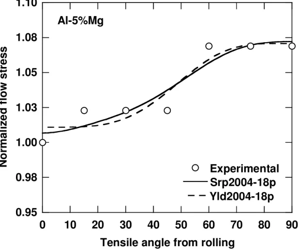
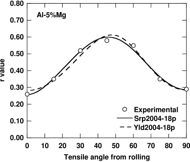
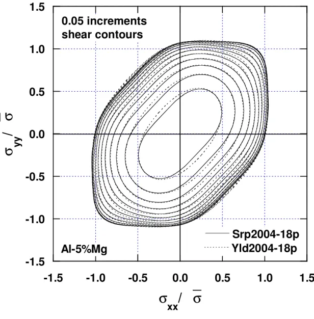
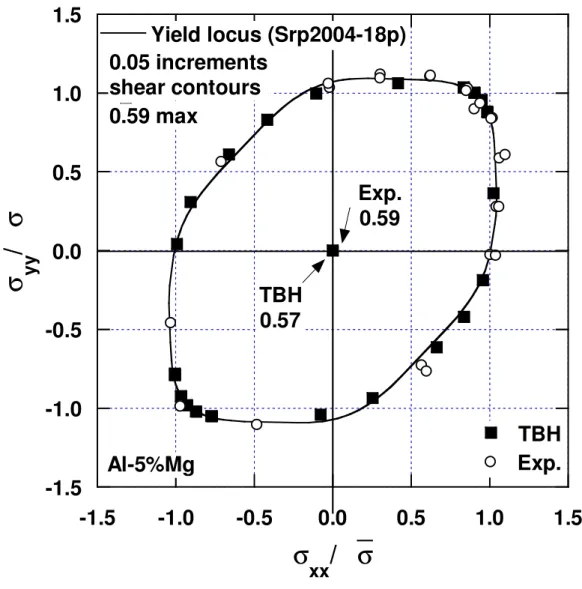
For the Al-5%Mg sheet sample, the anisotropic tensile properties given by the strain rate potential are shown in Figs. 3 and 4, and compared with properties predicted using the stress potential Yld2004-18p and experimental data. Figs. 3 and 4 show that the anisotropy of the tensile properties is well captured by Srp2004-18p. The anisotropic behaviors of the normalized uniaxial flow stress and r value as predicted with Srp2004-18p and Yld2004-Srp2004-18p are not strictly identical but very close to each other, suggesting that these potentials are pseudo-dual of each other. Fig. 5 represents the tri-component strain rate potential contours predicted with Srp2004-18p for constant normalized shear strain rates in steps of 0.05. In the same manner, the tri-component yield stress potential contours predicted with Yld2004-18p and Srp2004-18p for constant normalized shear stress in steps of 0.05 (based on the plastic work equivalence principle) are compared to each other in Fig. 6. Although not exactly identical, the general shapes of these yield surfaces are similar. Therefore, both shapes are likely to lead to similar plastic behaviors. Note that the yield stress potential contour at zero shear stress (yield locus) is also compared with experimental yield surface data (see Yoon et al., 2006) and results predicted with the Taylor-Bishop and Hill (TBH) crystal plasticity model in Fig. 7. The agreement between the experimental and TBH-predicted data with both Yld2004-18p and Srp2004-18p is excellent, thus validating the models.

TABLE 1

Al-5%Mg input data for the calculation of Srp2004-18p coefficients, corresponding weight for objective function and predicted values with Srp2004-18p after error minimization. Flow stresses are normalized by σ0. τ is the pure shear yield stress.

Srp2004-18p exponent b=1.33 (FCC material)

Input Weight Prediction1 Input weight Prediction2

In-plane xy 0

σ

1.000 1.00 1.0068 r0 0.26 0.75 0.258 15

σ

1.023 1.00 1.0119 r15 0.35 0.75 0.354 30

σ

1.023 1.00 1.0217 r30 0.52 0.75 0.514 45

σ

1.023 1.00 1.0374 r45 0.58 0.75 0.599 60

σ

1.069 1.00 1.0568 r60 0.55 0.75 0.524 75

σ

1.069 1.00 1.0695 r75 0.35 0.75 0.363 90

σ

1.069 1.00 1.0722 r90 0.29 0.75 0.287 b

σ

0.950 1.00 0.9493 rb 0.77 0.75 0.770 Out-of-plane yz 45(yz)

σ

1.0000 0.01 1.0268

τ

(yz) 0.5450 0.01 0.5450 Out-of-plane zx 45(zx)

σ

1.0000 0.01 1.0362

τ

(zx) 0.5450 0.01 0.5450 1

Maximum error δ =1.4% (out-of-plane data excluded)

2

Maximum error δ =5.7% (out-of-plane data excluded)

TABLE 2

Coefficients for Al-5%Mg sheet (exponent b=1.33) Potential Srp2004-18p, 4x105 iterations 12 b′ 0.126486 b′′₁₂ 1.230271 13 b′ 0.055184 b′′₁₃ 1.179809 21 b′ 1.581121 b′′₂₁ 1.260789 23 b′ 1.518793 b′′₂₃ 0.735545 31 b′ 0.940940 b′′₃₁ 1.291440 32 b′ 0.984856 b′′₃₂ 0.683715

TABLE 3

DP600 input data for the calculation of Srp2004-18p coefficients, corresponding weight for objective function and predicted values with Srp2004-18p after error minimization.

Flow stresses are normalized by σ0. τ is the pure shear yield stress. Srp2004-18p

exponent b=3 2 (BCC material)

Input weight Prediction1 Input weight Prediction2

In-plane 0

σ

1.000 1.00 0.9895 r0 0.86 0.75 0.857 15

σ

0.977 1.00 0.9922 r15 0.87 0.75 0.857 30

σ

1.000 1.00 1.0044 r30 1.01 0.75 0.996 45

σ

1.031 1.00 1.0097 r45 1.15 0.75 1.158 60

σ

0.987 1.00 1.0020 r60 1.20 0.75 1.191 75

σ

0.987 1.00 0.9921 r75 1.10 0.75 1.088 90

σ

0.997 1.00 0.9902 r90 1.04 0.75 1.039 b

σ

0.961 1.00 0.9594 rb 1.00 0.75 0.999 Out-of-plane yz

σ

45(yz) 1.000 0.01 1.0216

τ

(yz) 0.577 0.01 0. 5770 Out-of-plane zx

σ

45(zx) 1.000 0.01 1.0038

τ

(zx) 0.577 0.01 0. 5770 1

Maximum error δ =2.1% (out-of-plane data excluded)

2

Maximum error δ =1.4% (out-of-plane data excluded)

TABLE 4

Coefficients for DP600 sheet (exponent b=1.5) Potential Srp2004-18p, 4x105 iterations 12 b′ 1.671128 b′′₁₂ 0.886957 13 b′ 0.846769 b′′₁₃ 1.291898 21 b′ 0.616292 b′′₂₁ 0.232192 23 b′ 1.123290 b′′₂₃ 0.338996 31 b′ 0.525364 b′′₃₁ 1.057627 32 b′ 1.102594 b′′₃₂ 0.819647 44 b′ 1.038388 b′′₄₄ 1.038388 55 b′ 1.038388 b′′₅₅ 1.038388 66 b′ 1.427181 b′′₆₆ 0.454358

0.95

0.98

1.00

1.03

1.05

1.08

1.10

0

10

20

30

40

50

60

70

80

90

Experimental

Srp2004-18p

Yld2004-18p

N

o

rm

a

li

z

e

d

f

lo

w

s

tr

e

s

s

Tensile angle from rolling

Al-5%Mg

Fig. 3: Anisotropy of normalized uniaxial flow stress for Al-5%Mg sheet sample. Normalization with respect to RD tensile stress

0.00

0.10

0.20

0.30

0.40

0.50

0.60

0.70

0.80

0

10

20

30

40

50

60

70

80

90

Experimental

Srp2004-18p

Yld2004-18p

r

v

a

lu

e

Tensile angle from rolling

Al-5%Mg

-1.50

-1.00

-0.50

0.00

0.50

1.00

1.50

-1.50

-1.00

-0.50

0.00

0.50

1.00

1.50

Srp2004-18p

ε

y y

/

ε

ε

xx

/

ε

.

.

.

. .

Al-5%Mg

0.05 increments

shear contours

Fig. 5: Tri-component strain-rate potential predicted with Srp2004-18p for Al-5%Mg sheet sample.

-1.5

-1.0

-0.5

0.0

0.5

1.0

1.5

-1.5

-1.0

-0.5

0.0

0.5

1.0

1.5

Srp2004-18p

Yld2004-18p

σ

y

y

/

σ

σ

xx

/ σ

Al-5%Mg

0.05 increments

shear contours

Fig. 6: Tri-component yield surface predicted with Srp2004-18p and Yld2004-18p for Al-5%Mg sheet sample.

-1.5

-1.0

-0.5

0.0

0.5

1.0

1.5

-1.5

-1.0

-0.5

0.0

0.5

1.0

1.5

TBH

Exp.

Yield locus (Srp2004-18p)

σ

yy

/

σ

σ

xx

/

σ

Al-5%Mg

0.05 increments

shear contours

TBH

0.57

Exp.

0.59

0.59 max

Fig. 7: Yield loci predicted with Srp2004-18p and compared with experimental and crystal plasticity (TBH) predicted data for Al-5%Mg sheet sample.

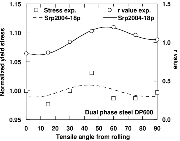
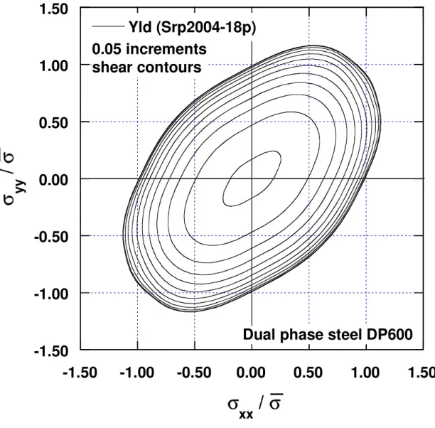
In Fig. 8, the anisotropy of uniaxial tension properties for the dual phase steel DP600 shows the ability of the developed strain rate potential to accurately describe the plastic behavior of a BCC material as well. Figs. 9 and 10 represents the corresponding tri-component strain rate and stress potential contours, respectively, predicted with

0.95

1.00

1.05

1.10

1.15

0.0

0.5

1.0

1.5

0

10

20

30

40

50

60

70

80

90

Stress exp.

Srp2004-18p

r value exp.

Srp2004-18p

N

o

rm

a

li

z

e

d

y

ie

ld

s

tr

e

s

s

r v

a

lu

e

Tensile angle from rolling

Dual phase steel DP600

Fig. 8: Anisotropy of tensile properties value predicted with Srp2004-18p for dual phase steel DP600 sheet sample.

-1.50

-1.00

-0.50

0.00

0.50

1.00

1.50

-1.50

-1.00

-0.50

0.00

0.50

1.00

1.50

Srp2004-18p

ε

y y

/

ε

ε

xx

/

ε

.

.

.

. .

0.05 increments

shear contours

Dual phase steel DP600

Fig. 9: Tri-component strain-rate potential predicted with Srp2004-18p for dual phase steel DP600 sheet sample.

-1.50

-1.00

-0.50

0.00

0.50

1.00

1.50

-1.50

-1.00

-0.50

0.00

0.50

1.00

1.50

Yld (Srp2004-18p)

σ

y y

/

σ

σ

xx

/

σ

|

0.05 increments

shear contours

Dual phase steel DP600

Fig. 10: Tri-component yield surface predicted with Srp2004-18p for dual phase steel DP600 sheet sample.

5.2. Application of Srp2006-18p

In a similar manner, the coefficients for Srp2006-18p in Eq. (4), were computed and their values are reported in Table 5 and 6 for Al-5%Mg and DP600 steel sheet samples, respectively. For Al-5%Mg, it was found that that the calculated tensile properties as well as the tri-component yield surface were strictly identical to those computed with Srp2004-18p. For DP600, the calculated tensile properties were very close to those obtained with Srp2004-18p. The tri-component yield surfaces for both potentials were

similar but not identical (compare Figs. 10 and 11). More work is needed to understand these small differences and to study and improve the anisotropy coefficient identification methods.

TABLE 5

Coefficients for Al-5%Mg sheet (exponent b=1.33) Potential Srp2006-18p, 4x105 iterations 12 b′ 1.837121 b′′₁₂ 0.169677 13 b′ 1.765692 b′′₁₃ 0.174579 21 b′ 0.587230 b′′₂₁ 1.604140 23 b′ 0.643928 b′′₂₃ 1.566223 31 b′ 0.807559 b′′₃₁ 0.807650 32 b′ 0.858777 b′′₃₂ 0.858874 44 b′ 1.005105 b′′₄₄ 1.005105 55 b′ 1.005105 b′′₅₅ 1.005105 66 b′ 1.289524 b′′₆₆ 0.863575 TABLE 6

Coefficients for DP600 sheet (exponent b=1.5) Potential Srp2006-18p, 4x105 iterations 12 b′ 0.907887 b′′₁₂ 0.909685 13 b′ 0.757080 b′′₁₃ 0.760076 21 b′ 0.927827 b′′₂₁ 0.924590 23 b′ 0.897922 b′′₂₃ 0.895522 31 b′ 1.506506 b′′₃₁ 0.773152 32 b′ 0.858450 b′′₃₂ 1.256440 44 b′ 1.038388 b′′₄₄ 1.038388 55 b′ 1.038388 b′′₅₅ 1.038388

-1.50

-1.00

-0.50

0.00

0.50

1.00

1.50

-1.50

-1.00

-0.50

0.00

0.50

1.00

1.50

Srp2006-18p

σ

y y

/

σ

σ

xx

/

σ

|

Dual phase steel DP600

Fig. 11: Tri-component yield surface predicted with Srp2006-18p for dual phase steel DP600 sheet sample.

6. SUMMARY

Anisotropic plastic strain-rate potentials were proposed for the description of plastic anisotropy in cubic materials. These potentials are valid for any 3-D strain rate state and their convexities were proven. It was shown that these potentials can reproduce the anisotropic plastic behavior of an aluminum alloy Al-5%Mg and DP600 dual phase steel sheet samples very well. These potentials can be very useful for finite element analysis and design codes, in particular those based on rigid plasticity, or for the approximation of crystal plasticity results.

ACKNOWLEDGEMENT

The authors of this paper would like to thank the Korea Science and Engineering Foundation (KOSEF) for sponsoring this research through the SRC/ERC Program of MOST/KOSEF (R11-2005-065).

REFERENCES

Arminjon, M., Bacroix, B., 1991. On Plastic Potentials for Anisotropic Metals and Their Derivation From the Texture Function. Acta Mechanica 88, 219-243.

Arminjon, M., Imbault, D., Bacroix, B., Raphanel, J.L., 1994. A fourth-order plastic potential for anisotropic metals and its analytical calculation from the texture function. Acta Mech. 107, 33-51.

Bacroix, B., Gilormini, P., 1995. Finite-element simulations of earing in polycrystalline materials using a texture-adjusted strain-rate potential. Model. Simul. Mater. Sci. Eng. 3, 1-21.

Barlat, F., Aretz, H., Yoon, J.W., Karabin, M.E., Brem, J.C., Dick, R.E., 2005. Linear transformation-based anisotropic yield functions. Int. J. Plasticity 21, 1009–1039. Barlat, F., Brem, J.C., Yoon, J.W., Chung, K., Dick, R.E., Choi, S.-H., Pourboghrat, F.,

Chu, E., Lege, D.J., 2003. Plane stress yield function for aluminum alloy sheets. Int. J. Plasticity 19, 1297-1319.

Barlat, F., Brem, J.C., Yoon, J.W., Dick, R.E., Choi, S.H., Chung, K., Lege, D.J., 2000. Constitutive modeling for aluminum sheet forming simulations, in Plastic and Viscoplastic Response of Materials and Metal Forming, Proc. 8th Intern. Symposium on Plasticity and its Current Applications, Whistler, Canada, July 2000, Ed. Khan, A.S, Zhang, H. and Yuan, Y., Neat Press, Fulton, Maryland, pp. 591-593.

Barlat, F., Chung, K., 1993. Anisotropic potentials for plastically deformation metals. Modelling Simul. Mater. Sci. Engng. 1, 403-416.

Barlat, F., Chung, K., 2005. Anisotropic strain rate potential for aluminum alloy plasticity. In: Proc. 8th ESAFORM Conference on Material Forming, Cluj-Napoca, Romania, April 2005. Banabic, D., (Ed.), The Publishing House of the Romanian Academy, Bucharest, pp. 415-418.

Barlat, F., Chung, K., Richmond, O., 1993. Strain rate potential for metals and its application to minimum work path calculations. Int. J. Plasticity 9, 51-63.

materials. Int. J. Plasticity 7, 693-712.

Barlat, F., Maeda, Y., Chung, K., Yanagawa, M., Brem, J. C., Hayashida, Y., Lege, D. J., Matsui, K., Murtha, S.J., Hattori, S., Becker, R.C., Makosey, S., 1997. Yield function development for aluminum alloy sheets. J. Mech. Phys. Solids 45, 1727-1763.

Chung, K., Richmond, O., 1992a. Ideal forming, Part I: Homogeneous deformation with minimum plastic work. Int. J. Mech. Sci. 34(7), 575-591.

Chung, K., Richmond, O., 1992b. Ideal Forming, Part II: Sheet forming with optimum deformation. Int. J. Mech. Sci., 34, 617-633.

Chung, K., Shah, K., 1992. Finite element simulation of sheet metal forming for planar anisotropic metals. Int. J. Plasticity 8, 453-476.

Chung, K., Richmond, O., 1993. A deformation theory of plasticity based on minimum work paths. Int. J. Plasticity 9, 907-920.

Chung, K., Richmond, O., 1994. Mechanics of ideal forming. J. Appl. Mech., ASME, 61, 176.

Chung, K., Lee, S.Y., Barlat, F., Keum, Y.T., and Park, J.M., 1996. Finite element simulation of sheet forming based on a planar anisotropic strain-rate potential. Int. J. Plasticity 12(1), 93-115.

Chung, K., Barlat, F., Brem, J.C., Lege, D.J., Richmond, O., 1997. Blank shape design for a planar anisotropic sheet based on ideal forming design theory and FEM analysis. Int. J. Mech. Sci., 39(1), 105-120.

Chung, K., Barlat, F., Richmond, O., Yoon, J.W., 1999. Blank design for a sheet forming application using the anisotropic strain-rate potential Srp98. The integration of Material, Process and Product Design, Zabaras et al. (Eds.), Balkema, Rotterdam. 213-219.

Chung, K., Yoon, J.W., Richmond, O., 2000. Ideal sheet forming with frictional constraints. Int. J. Plasticity, 16, 595-610.

Chung, K., 2004. Forming analysis and design for hydroforming. Continuum Scale Simulation of Engineering Materials, WILEY-VCH Verlag GmbH & Co. KGaA. 763-775

Chung, K., Lee, M.-G., Kim, D., Kim, C., Wenner, M.L., Barlat, F., 2005. Spring-back evaluation of automotive sheets based on isotropic-kinematic hardening laws and non-quadratic anisotropic yield functions. Part I: Theory and formulation. Int. J. Plasticity 21, 861–882.

Fortunier, R., 1989. Dual potentials and extremum work principles in single crystal plasticity. J. Mech. Phys. Solids 37, 779.

Germain, Y., Chung, K., Wagoner, R.H., 1989. A rigid-visco-plastic finite element program for sheet metal forming analysis. Int. J. Mech. Sci. 31., 1-24.

Hill, R., 1948. A theory of the yielding and plastic flow of anisotropic metals. Proc. R. Soc. Lond., A193, 281.

Hill, R., 1979. Theoretical plasticity of textured aggregates. Math. Proc. Camb. Phil. Soc. 85, 179.

Hill, R., 1987. Constitutive dual potentials in classical plasticity. J. Mech. Phys. Solids 35, 23.

Hiwatashi, S., Van Bael, A., Van Houtte, P., Teodosiu C., 1997. Modelling of plastic anisotropy based on texture and dislocation structure. Comp. Mat. Science 9, 274. Hu, J.G., Jonas, J.J., Ishikawa, T., 1998, FEM simulation of the forming of textured

aluminum sheets. Mat. Science Engng A, 256, 51.

Kim, K.J., Kim, D., Chi, S.H., Chung, K., Shin, K.S., Barlat, F., Oh, K.H., Youn, J.R., 2003a, Formability of AA5182/polypropylene/AA5182 sandwich sheet. J. Mater. Process. Technol. 139, 1-7.

Kim, D., Chung, K., Barlat, F., Youn, J.R., Kang, T.J., 2003b, Non-quadratic plane-stress anisotropic strain-rate potential, Proceedings of the Sixth International Symposium on Microstructures and Mechanical Properties of New Engineering Materials (IMMM 2003), Wuhan, China, Oct. 26-Nov. 1, 2003, pp.46-51.

Lee, M.-G., Kim, D., Kim, C., Wenner, M.L., Wagoner, R.H., Chung, K., 2005a. Spring-back evaluation of automotive sheets based on isotropic-kinematic hardening laws and non-quadratic anisotropic yield functions, Part II: Characterization of material properties. Int. J. Plasticity 21, 883–914.

Lee, M.-G., Kim, D., Kim, C., Wenner, M.L., Wagoner, R.H., Chung, K., 2005b. Spring-back evaluation of automotive sheets based on isotropic-kinematic hardening laws and non-quadratic anisotropic yield functions, Part III: Application. Int. J. Plasticity 21, 915-953.

Lee, S.Y., Keum, Y.T., Chung, K., Park, J.M., Barlat, F., 1997. Three-dimensional finite-element method simulations of stamping processes for planar anisotropic sheet metals. Int. J. Mech. Sci. 39(10), 1181-1198.

Li, S., Hoferlin, E., Van Bael, A, 2001. Application of a texture-based plastic potential in earing prediction of an IF steel. Advanced Engineering Materials 3, 990-994. Rockafellar, R.T., 1970. Convex Analysis. Princeton University Press, Princeton, NY. Ryou, H., Chung, K., Yoon, J.-W., Han, C.-S., Youn, J.R., Kang, T.J., 2005.

Incorporation of sheet-forming effects in crash simulations using ideal forming theory and hybrid membrane and shell method. Journal of Manufacturing Science and Engineering ASME, 127, 182-192.

Szabó, L., Jonas J.J., 1995. Consistent tangent operator for plasticity models based on the plastic strain rate potential, Comp. Met. Applied Mech. Engng. 128, 315.

Van Bael, A., Van Houtte, P., 2002. Convex fourth and sixth-order plastic potentials derived form crystallographic texture. In: Cescotto, S. (Ed.), Non Linear Mechanics of Anisotropic Materials. Proceedings of the Sixth European Mechanics of Materials Conference (EMMC6), Liege, Belgium, September 2002. University of Liege, pp.

for anisotropic materials. Int. J. Plasticity 20, 1505-1524.

Yoon, J.W., Song, I.S., Yang, D.Y., Chung, K., Barlat, F., 1995. Finite element method for sheet forming based on an anisotropic strain-rate potential and the convected coordinate system. Int. J. Mech. Sci. 37, 733-752.

Yoon, J.W., Barlat, F., Chung, K., Pourboghrat, F., Yang, D.Y., 1998, Influence of initial back stress on the earing prediction of drawn cups for planar anisotropic aluminum alloys. Journal of Material Processing Technology 80-81, 433-437

Yoon, J.W., Chung, K., Barlat, F., Allison, B.T., Richmond, O., 1999, Aluminum sheet forming design based on the non-quadratic strain rate potential SRP98. Proceedings of NUMISHEET’99, Besancon, France, September 13-17, 103-108.

Yoon, J.W., Yang, D.Y., Chung, K., 1999a. Elasto-plastic finite element method based on incremental deformation theory and continuum based shell elements for planar anisotropic sheet materials. Comp. Methods Appl. Mech. Eng. 174, 23-56.

Yoon, J.W., Yang, D.Y., Chung, K., 1999b. A general elasto-plastic finite element formulation based on incremental deformation theory for planar anisotropy and its application to sheet metal forming. Int. J. Plasticity 15, 35-68.

Yoon, J.W., Barlat, F., Chung, K., Pourboghrat, F., Yang, D.Y., 2000. Earing predictions based on asymmetric nonquadratic yield function. Int. J. Plasticity 16, 1075-1104. Yoon, J.-W., Chung, K., Pourboghrat, Farhng., Shah, K.N., Chu, E.W., 2002. Preform

design for hydroforming processes based on ideal forming design theory. Proceedings of NUMISHEET’02, Jeju Island, Korea, October 21-25, 2002, pp. 385-390.

Yoon, J.W., Barlat, F., Dick, R.E., Chung, K., Kang, T.J., 2004. Plane stress yield function for aluminum alloy sheets, Part II: FE formulation and its implementation. Int. J. Plasticity 20, 495-522.

Yoon, J.W., Barlat, F., Dick, R.E., 2000. Sheet metal forming simulation for aluminum alloy sheets, In Sheet Metal Forming Simulation: Sing-Tang 65th Anniversary Volume, SAE paper 2000-01-0774, Society of Automotive Engineer, SAE, 67-72. Yoon, J.W., Barlat, F., Dick, R.E., Karabin, M.E., 2006. Prediction of six or eight ears in

a drawn cup based on a new anisotropic yield function. Int. J. Plasticity 22, 174-193. Zhou, D., Wagoner, R.H., 1994. A numerical method for introducing an arbitrary yield function into rigid-viscoplastic FEM programs. Int. J. Numerical Methods in Eng. 37, 3467-3486.

Zhou, Y., Jonas J.J., Savoie J., Makinde A., MacEwen S.R., 1998. Effect of texture on earing in FCC metals: Finite element simulations, Int. J. Plasticity 14, 117.

Ziegler, H., 1977. An Introduction to Thermodynamics. North Holland Publishing Company, Amsterdam.