EUROPEAN ORGANISATION FOR NUCLEAR RESEARCH (CERN)
Submitted to: EPJC CERN-PH-EP-2015-294
2nd June 2016
Reconstruction of hadronic decay products of tau leptons with the
ATLAS experiment
The ATLAS Collaboration
Abstract
This paper presents a new method of reconstructing the individual charged and neutral had-rons in tau decays with the ATLAS detector. The reconstructed hadhad-rons are used to classify the decay mode and to calculate the visible four-momentum of reconstructed tau candidates, significantly improving the resolution with respect to the calibration in the existing tau re-construction. The performance of the reconstruction algorithm is optimised and evaluated using simulation and validated using samples of Z → ττ and Z(→ µµ)+jets events selected from proton–proton collisions at a centre-of-mass energy √s = 8 TeV, corresponding to an integrated luminosity of 5 fb−1.
1 Introduction
Final states with hadronically decaying tau leptons play an important part in the physics programme of the ATLAS experiment [1]. Examples from Run 1 (2009–2013) of the Large Hadron Collider (LHC) [2] are measurements of Standard Model processes [3–7], Higgs boson searches [8], including models with extended Higgs sectors [9–11], and searches for new physics phenomena, such as supersymmetry [12– 14], new heavy gauge bosons [15] and leptoquarks [16]. These analyses depended on robust tau recon-struction and excellent particle identification algorithms that provided suppression of backgrounds from jets, electrons and muons [17].
With the discovery of a Higgs boson [18,19] and evidence for the Higgs-boson Yukawa coupling to tau leptons [8, 20], a key future measurement will be that of the CP mixture of the Higgs boson via spin effects in H → ττ decays [21–23]. This measurement relies on high-purity selection of the τ− → π−ν, τ− → π−π0ν and τ− → π−π+π−ν decays, as well as the reconstruction of the individual charged and neutral pion four-momenta. The tau reconstruction used in ATLAS throughout Run 1 (here denoted as “Baseline”), however, only differentiates tau decay modes by the number of charged hadrons and does not provide access to reconstructed neutral pions.
This paper presents a new method (called “Tau Particle Flow”) of reconstructing the individual charged and neutral hadrons in tau decays with the ATLAS detector. Charged hadrons are reconstructed from their tracks in the tracking system. Neutral pions are reconstructed from their energy deposits in the calorimeter. The reconstructed hadrons, which make up the visible part of the tau decay (τhad−vis), are used to classify the decay mode and to calculate the four-momentum of reconstructed τhad−viscandidates. The superior four-momentum resolution from the tracking system compared to the calorimeter, for charged hadrons with transverse momentum (pT) less than ∼100 GeV, leads to a significant improvement in the tau energy and directional resolution. This improvement, coupled with the ability to better identify the hadronic tau decay modes, could lead to better resolution of the ditau mass reconstruction [24]. The performance of the Tau Particle Flow is validated using samples of real hadronic tau decays and jets in Z+jets events selected from data. The samples correspond to 5 fb−1of data collected during proton–proton collisions at a centre-of-mass energy of √s= 8 TeV, which was the amount of data reprocessed using Tau Particle Flow. While similar concepts for the reconstruction of hadronic tau decays have been employed at other experiments [25–31], the Tau Particle Flow is specifically designed to exploit the features of the ATLAS detector and to perform well in the environment of the LHC.
The paper is structured as follows. The ATLAS detector, event samples, and the reconstruction of physics objects used to select τhad−vis candidates from the 8 TeV data are described in Section2. The properties of τhad−vis decays and the Tau Particle Flow method are described in Section3, including its concepts (Section3.1), neutral pion reconstruction (Section3.2), reconstruction of individual photon energy de-posits (Section3.3), decay mode classification (Section3.4) and τhad−visfour-momentum reconstruction (Section3.5). Conclusions are presented in Section4.
2 ATLAS detector and event samples
2.1 The ATLAS detectorThe ATLAS detector [1] consists of an inner tracking system surrounded by a superconducting solenoid, electromagnetic (EM) and hadronic (HAD) calorimeters, and a muon spectrometer. The inner detector is immersed in a 2 T axial magnetic field, and consists of pixel and silicon microstrip detectors inside a transition radiation tracker, which together provide charged-particle tracking in the region |η| < 2.5.1 The EM calorimeter is based on lead and liquid argon as absorber and active material, respectively. In the central rapidity region, the EM calorimeter is divided radially into three layers: the innermost layer (EM1) is finely segmented in η for optimal γ/π0separation, the layer next in radius (EM2) collects most of the energy deposited by electron and photon showers, and the third layer (EM3) is used to correct leakage beyond the EM calorimeter for high-energy showers. A thin presampler layer (PS) in front of EM1 and in the range |η| < 1.8 is used to correct showers for upstream energy loss. Hadron calorimetry is based on different detector technologies, with scintillator tiles (|η| < 1.7) or liquid argon (1.5 < |η| < 4.9) as active media, and with steel, copper, or tungsten as absorber material. The calorimeters provide coverage within |η| < 4.9. The muon spectrometer consists of superconducting air-core toroids, a system of trigger chambers covering the range |η| < 2.4, and high-precision tracking chambers allowing muon momentum measurements within |η| < 2.7. A three-level trigger system is used to select interesting events [32]. The first-level trigger is implemented in hardware and uses a subset of detector information to reduce the event rate to a design value of at most 75 kHz. This is followed by two software-based trigger levels which together reduce the average event rate to 400 Hz.
2.2 Physics objects
This section describes the Baseline τhad−visreconstruction and also the reconstruction of muons and the missing transverse momentum, which are required for the selection of samples from data. Tau Particle Flow operates on each reconstructed Baseline tau candidate to reconstruct the charged and neutral had-rons, classify the decay mode and to provide an alternative τhad−vis four-momentum. Suppression of backgrounds from other particles misidentified as τhad−vis is achieved independently of the Tau Particle Flow.
The Baseline τhad−vis reconstruction and energy calibration, and the algorithms used to suppress back-grounds from jets, electrons and muons are described in detail in Ref. [17]. Candidates for hadronic tau decays are built from jets reconstructed using the anti-ktalgorithm [33,34] with a radius parameter value of 0.4. Three-dimensional clusters of calorimeter cells calibrated using a local hadronic calibration [35, 36] serve as inputs to the jet algorithm. The calculation of the τhad−visfour-momentum uses clusters within the core region (∆R < 0.2 from the initial jet-axis). It includes a final tau-specific calibration derived from simulated samples, which accounts for out-of-cone energy, underlying event, the typical composition of hadrons in hadronic tau decays and contributions from multiple interactions occurring in the same and neighbouring bunch crossings (called pile-up). Tracks reconstructed in the inner detector are matched 1ATLAS uses a right-handed coordinate system with its origin at the nominal interaction point (IP) in the centre of the detector
Process Generator PDFs UE tune
Z →ττ Pythia 8 [43] CTEQ6L1 [44] AU2 [45]
W →µν Alpgen [46]+Pythia 8 CTEQ6L1 Perugia [47]
W →τν Alpgen+Pythia 8 CTEQ6L1 Perugia
Z →µµ Alpgen+Pythia 8 CTEQ6L1 Perugia
t¯t MC@NLO [48–50]+Herwig [51,52] CT10 [53] AUET2 [45]
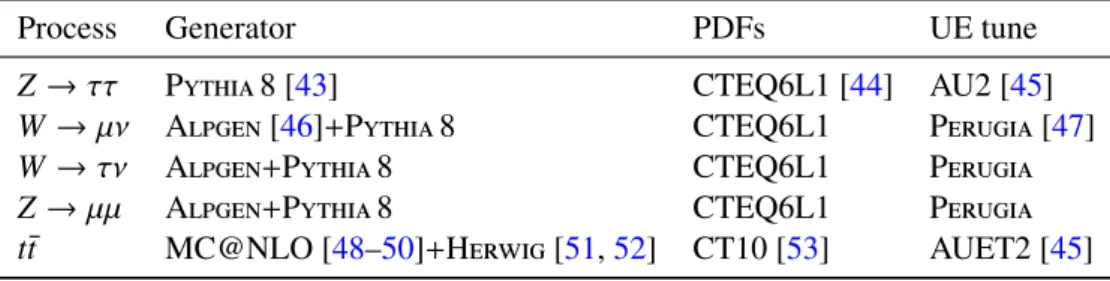
Table 1: Details regarding the simulated samples of pp collision events. The following information is provided for each sample: the generator of the hard interaction, parton shower, hadronisation and multiple parton interactions; the set of parton distribution functions (PDFs) and the underlying event (UE) tune of the Monte Carlo.
to the τhad−viscandidate if they are in the core region and satisfy the following criteria: pT > 1 GeV, at least two associated hits in the pixel layers of the inner detector, and at least seven hits in total in the pixel and silicon microstrip layers. Furthermore, requirements are imposed on the distance of closest approach of the tracks to the tau primary vertex in the transverse plane, |d0|< 1.0 mm, and longitudinally, |z0sin θ| < 1.5 mm. The τhad−vis charge is reconstructed from the sum of the charges of the associated tracks.
Backgrounds for τhad−vis candidates originating from quark- and gluon-initiated jets are discriminated against by combining shower shape and tracking information in a multivariate algorithm that employs boosted decision trees (BDTs) [37]. The efficiency of the jet discrimination algorithm has little depend-ence on the pTof the τhad−viscandidates (evaluated using candidates with pT > 15 GeV) or on the number of reconstructed primary vertices, which is correlated to the amount of pile-up, and has been evaluated up to a maximum of 25 primary vertices per event. All τhad−viscandidates are required to have pT > 15 GeV, to be in the fiducial volume of the inner detector, |η| < 2.5, and to have one or three associated tracks. They must also meet jet discrimination criteria, corresponding to an efficiency of about 55% (40%) for simulated τhad−vis with one (three) charged decay products [17], leading to a rate of false identification for quark- and gluon-initiated jets of below a percent. A discriminant designed to suppress candidates arising from the misidentification of electrons [17] is also applied.
Muons are reconstructed using tracks in the muon spectrometer and inner detector [38]. The missing transverse momentum is computed from the combination of all reconstructed and fully calibrated physics objects and the remaining clustered energy deposits in the calorimeter not associated with those ob-jects [39].
2.3 Event samples and selection
The optimisation and measurement of the τhad−visreconstruction performance requires Monte Carlo sim-ulated events. Samples of simsim-ulated pp collision events at √s = 8 TeV are summarised in Table1. Tau decays are provided by Z → ττ events. The sophisticated tau decay option of Pythia 8 is used, which provides fully modelled hadronic decays with spin correlations [40]. Tau decays in the t¯t sample are gen-erated by Tauola [41]. Photon radiation is performed by Photos [42]. Single-pion samples are also used, in which the pions originate from the centre of the ATLAS detector and are generated to have a uniform distribution in φ and η (|η| < 5.5) and also in log(E) (200 MeV < E < 2 TeV).
The response of the ATLAS detector is simulated using Geant4 [54,55] with the hadronic-shower model QGSP_BERT [56,57]. The parameters of the underlying event (UE) simulation were tuned using collision data. Simulated pp collision events are overlaid with additional minimum-bias events generated with Pythia 8 to account for the effect of pile-up. When comparing to the data, the simulated events are reweighted so that the distribution of the number of pile-up interactions matches that in the data. The simulated events are reconstructed with the same algorithm chain as used for the collision data.
Samples of τhad−vis candidates are selected from the data using a tag-and-probe approach. Candidates originating from hadronic tau decays and jets are obtained by selecting Z → ττ and Z(→ µµ)+jets events, respectively. The data were collected by the ATLAS detector during pp collisions at √s= 8 TeV. The sample corresponds to an integrated luminosity of 5 fb−1after making suitable data quality requirements for the operation of the tracking, calorimeter, and muon spectrometer subsystems. The data have a max-imum instantaneous luminosity of 7 · 1033cm−2s−1and an average number of 19 pp interactions in the same bunch crossing.
The Z → ττ tag-and-probe approach follows Ref. [17]; events are triggered by the presence of a muon from a leptonic tau decay (tag) and must contain a τhad−viscandidate (probe) with pT > 20 GeV, which is used to evaluate the tau reconstruction performance. The τhad−visselection criteria described in Section2.2 are used. In addition the τhad−vismust have unit charge which is opposite to that of the muon. A discrim-inant designed to suppress candidates arising from the misidentification of muons [17] is also applied to increase signal purity. The invariant mass of the muon and τhad−vis, m(µ, τhad−vis), is required to be in the range 50 GeV < m(µ, τhad−vis) < 85 GeV, as expected for Z → ττ decays. The background is dominated by multijet and W(→ µν)+jets production and is estimated using the techniques from Ref. [7].
The Z(→ µµ)+jets tag-and-probe approach follows Ref. [58], with the following differences: both muons are required to have pT > 26 GeV, the dimuon invariant mass must be between 81 and 101 GeV, and the highest-pTjet is selected as a probe τhad−viscandidate if it satisfies the τhad−visselection criteria described in Section2.2but with pT > 20 GeV and without the electron discriminant. In this approach, two more steps are made when comparing simulated events to the data. Before the τhad−visselection, the simulated events are reweighted so that the pT distribution of the Z boson matches that in data. After the full event selection, the overall normalisation of the simulation is scaled to that in the data.
3 Reconstruction of the
τ
had−visOver 90% of hadronic tau decays occur through just five dominant decay modes, which yield one or three charged hadrons (h±), up to two neutral pions (π0) and a tau neutrino. The neutrino goes undetected and is omitted in further discussion of the decay modes. Table2gives the following details for each of the five decay modes: the branching fraction, B; the fraction of simulated τhad−vis candidates that pass the τhad−vis selection described in Section2.2without the jet and electron discrimination, A · εreco; and the fraction of those that also pass the jet and electron discrimination, εID. The h±’s are predominantly π±’s with a minor contribution from K±’s. The modes with two or three pions proceed mainly through the intermediate ρ or a1resonances, respectively. The h±’s are sufficiently long-lived that they typically interact with the detector before decaying and are therefore considered stable in the Tau Particle Flow. The π0’s decay almost exclusively to a pair of photons. Approximately half of the photons convert into
Decay mode B [%] A ·εreco[%] εID[%] h± 11.5 32 75 h±π0 30.0 33 55 h±≥2π0 10.6 43 40 3h± 9.5 38 70 3h±≥1π0 5.1 38 46
Table 2: Five dominant τhad−visdecay modes [59]. Tau neutrinos are omitted from the table. The symbol h±stands
for π± or K±. Decays involving K± contribute ∼3% to the total hadronic branching fraction. Decays involving
neutral kaons are excluded. The branching fraction (B), the fraction of generated τhad−vis’s in simulated Z → ττ
events that are reconstructed and pass the τhad−vis selection described in Section2.2without the jet and electron
discrimination (A·εreco) and the fraction of those τhad−viscandidates that also pass the jet and electron discrimination
(εID) for each decay mode are given.
energy carried by visible decay products is mode dependent and the response of the calorimeter to h±’s and π0’s is different, both of which impact the efficiency of the τhad−vispTrequirement. The efficiency of the track association is also dependent on the number of h±’s and to a lesser extent the number of π0’s, which can contribute tracks from conversion electrons.
The goal of the Tau Particle Flow is to classify the five decay modes and to reconstruct the individual h±’s and π0’s. The performance is evaluated using the energy and directional residuals of π0and τhad−vis and the efficiency of the τhad−visdecay mode classification. The η and φ residuals are defined with respect to the generated values: η − ηgen and φ − φgen, respectively. For ET, the relative residual is defined with respect to the generated value ET/ETgen. The core and tail resolutions for η, φ and ETare defined as half of the 68% and 95% central intervals of their residuals, respectively. Decays into higher-multiplicity states are accommodated by including modes with more than two π0’s in the h±≥2π0 category and more than one π0in the 3h±≥1π0 category. Decays with more than three charged hadrons are not considered. No attempt is made to reconstruct neutral kaons or to separate charged kaons from charged pions.
3.1 Concepts of the Tau Particle Flow method
The main focus of the Tau Particle Flow method is to reconstruct τhad−vis’s with pT values between 15 and 100 GeV, which is the relevant range for tau leptons produced in decays of electroweak and SM Higgs bosons. In this case the hadrons typically have pT lower than 20 GeV (peaked at ∼4 GeV) and have an average separation of∆R ≈ 0.07. The h±’s are reconstructed using the tracking system, from which the charge and momentum are determined. Each track associated with the τhad−vis candidate in the core region is considered to be a h± and the π±mass hypothesis is applied. Approximately 2% of the selected τhad−vis’s have a misclassified number of h±’s. Overestimation of the number of h±’s is primarily due to additional tracks from conversion electrons, which are highly suppressed by the strict track selection criteria described in Section2.2. Underestimation of the number of h±’s is primarily caused by tracking inefficiencies (∼10% for charged pions with pT > 1 GeV [1]), which arise from interactions of the h±’s with the beampipe or detector material. The h±’s also produce a shower in the calorimeter from which their energy and direction can be determined, but the tracker has a better performance in the relevant momentum range. The shower shapes of h±’s are also highly irregular, with a typical width of 0.02 <∆R < 0.07 in the EM calorimeter, combined with large fluctuations in the fractional energy depositions in the layers of the calorimeter. The π0’s are reconstructed from their energy deposits in
the EM calorimeter. The main challenge is to disentangle their energy deposits from h±showers, which have a width similar to the average separation between hadrons. The photons from π0decays are highly collimated, with a typical separation of 0.01 <∆R < 0.03. The majority of the π0energy is reconstructed in a single cluster in the EM calorimeter. Compared to h±’s, π0 showers are smaller and more regular, leaving on average 10%, 30% and 60% of their energy in PS, EM1 and EM2, respectively. Almost no π0 energy is deposited beyond EM2, so EM3 is considered part of the HAD calorimeter in Tau Particle Flow. The characteristic shower shapes and the kinematics of h±’s and π0’s are used to identify π0’s and to classify the tau decay mode.
In the following sections, the individual steps of the Tau Particle Flow method for τhad−visreconstruction are described. The first step is the reconstruction and identification of neutral pions. Next, energy deposits from individual photons in the finely segmented EM1 layer are reconstructed to identify cases where two π0’s are contained within a single cluster. The decay mode is then classified by exploiting the available information from the reconstructed h±’s and π0’s and the photons reconstructed in EM1. Following the decay mode classification, the τhad−visfour-momentum is reconstructed from the individual hadrons and then combined with the Baseline energy calibration to reduce tails in the ET residual distribution. The performance of the Tau Particle Flow is evaluated using τhad−vis candidates from simulated Z → ττ events.
3.2 Reconstruction and identification of neutral pions
The reconstruction of neutral pion candidates (π0cand) within hadronic tau decays using the Tau Particle Flow proceeds as follows. First, π0cand’s are created by clustering cells in the EM calorimeter in the core region of the τhad−vis. In the next step, the π0candenergy is corrected for contamination from h±’s. To do this, the energy that each h±deposits in the EM calorimeter (EEMh± ) is estimated as the difference between the energy of the h± from the tracking system (Etrkh±) and the energy deposited in the HAD calorimeter which is associated with the h±(EhHAD± ): EhEM± = Ehtrk± − EHADh± . To calculate EhHAD± , all clustered energy deposits in the HAD calorimeter in the core region are assigned to the closest h±, determined using the track position extrapolated to the calorimeter layer that contains most of the cluster energy. The EhEM± of each h±is then subtracted from the energy of the closest π0candif it is within∆R = 0.04 of the h±.
At this stage, many of the π0cand’s in reconstructed hadronic tau decays do not actually originate from π0’s, but rather from h±remnants, pile-up or other sources. The purity of π0
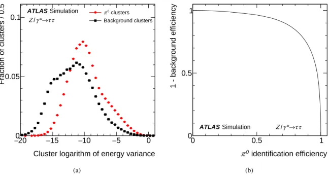
cand’s is improved by applying a minimum pT requirement and an identification criterion designed to reject π0cand’s not from π0’s. The pT thresholds are in the range 2.1–2.7 GeV. After the pT requirement the background is dominated by h±remnants. The π0 identification uses a BDT and exploits the properties of the π0candclusters, such as the energy density and the width and depth of the shower. The variables used for π0candidentification are described in Table3. The BDT is trained using τhad−vis’s that have only one h±, and which are produced in simulated Z → ττ events. The π0cand’s are assigned to signal or background based on whether or not they originated from a generated π0. Figure1(a) shows signal and background distributions for the logarithm of the second moment in energy density, which is one of the more important identification variables. The discriminating power of the π0identification is quantified by comparing the efficiency of signal and background π0cand’s to pass thresholds on the identification score, as shown in Fig.1(b). The pT and identification score thresholds are optimised in five |η| ranges, corresponding to structurally different
Cluster pseudorapidity, |ηclus|
Magnitude of the energy-weighted η position of the cluster Cluster width, hr2iclus
Second moment in distance to the shower axis Clusterη width in EM1, hη2
EM1i clus
Second moment in η in EM1 Clusterη width in EM2, hη2
EM2i clus
Second moment in η in EM2 Cluster depth,λclus
centre
Distance of the shower centre from the calorimeter front face measured along the shower axis
Cluster PS energy fraction, fclus PS Fraction of energy in the PS
Cluster core energy fraction, fcoreclus
Sum of the highest cell energy in PS, EM1 and EM2 divided by the total energy Cluster logarithm of energy variance, loghρ2iclus
Logarithm of the second moment in energy density Cluster EM1 core energy fraction, fclus
core,EM1
Energy in the three innermost EM1 cells divided by the total energy in EM1 Cluster asymmetry with respect to track, Aclus
track
Asymmetry in η–φ space of the energy distribution in EM1 with respect to the ex-trapolated track position
Cluster EM1 cells, Nclus EM1
Number of cells in EM1 with positive energy Cluster EM2 cells, Nclus
EM2
Number of cells in EM2 with positive energy
Table 3: Cluster variables used for π0
candidentification. The variables |η
clus|, hr2iclus, λclus
centre, fcoreclusand loghρ2iclusare
taken directly from the cluster reconstruction [36]. To avoid confusion with other variables used in tau reconstruc-tion, the superscript clus has been added to each variable.
The h± and π0counting performance is depicted in Fig.2by a decay mode classification matrix which shows the probability for a given generated mode to be reconstructed as a particular mode. Only τhad−vis decays that are reconstructed and pass the selection described in Section 2.2 are considered (corres-ponding efficiencies are given in Table2). The total fraction of correctly classified tau decays (diagonal fraction) is 70.9%. As can be seen, for τhad−vis’s with one h±, the separation of modes with and without π0’s is quite good, but it is difficult to distinguish between h±π0and h±≥2π0. The largest contributions to the misclassification arise from h±≥2π0decays where one of the π0’s failed selection or where the energy deposits of both π0’s merge into a single cluster. It is also difficult to distinguish between the 3h± and 3h±≥1π0modes because the π0’s are typically soft with large overlapping h±deposits.
Cluster logarithm of energy variance 20 − −15 −10 −5 0 Fraction of clusters / 0.5 0 0.05
0.1 ATLAS SimulationZ/γ*→ττ clusters
0 π Background clusters (a) identification efficiency 0 π 0 0.5 1 1 - background efficiency 0 0.5 1 ATLAS Simulation Z/γ*→ττ (b) Figure 1: (a) Distribution of the logarithm of the second moment in energy density of π0
candclusters that do (signal)
or do not (background) originate from π0’s, as used in the π0identification. (b) 1 − efficiency for background π0 cand’s
vs. the efficiency for signal π0
cand’s to pass thresholds on the π
0identification score. The π0
cand’s in both figures are
associated with τhad−vis’s selected from simulated Z → ττ events.
88.6 16.9 5.6 1.4 0.5
9.7 67.5 50.9 0.7 2.1
1.2 12.4 39.6 0.2 0.7
0.2 0.6 0.4 86.8 41.5
0.2 2.5 3.5 11.0 55.3
Generated decay mode ± h h±π0 π0 2 ≥ ± h 3h± 3h±≥1π0
Reconstructed decay mode
± h 0 π ± h 0 π 2 ≥ ± h ± h 3 0 π 1 ≥ ± h 3 ATLAS Simulation reconstruction) 0 π
Tau Particle Flow ( Z/γ*→ττ Diagonal fraction: 70.9%
Figure 2: Decay mode classification efficiency matrix showing the probability for a given generated mode to be reconstructed as a particular mode by the Tau Particle Flow after π0reconstruction in simulated Z → ττ events.
De-Two alternative methods for π0reconstruction were also developed. In the first method (Pi0Finder) the number of π0’s in the core region is first estimated from global tau features measured using calorimetric quantities and the momenta of the associated h±tracks. Clusters in the EM calorimeter are then chosen as π0cand’s using a π0 likeness score based on their energy deposition in the calorimeter layers and the τhad−vistrack momenta. The likeness score does not exploit cluster moments to the same extent as the π0 identification of the Tau Particle Flow and cluster moments are not used at all to estimate the number of π0. This method was used to calculate variables for jet discrimination in Run 1 [17], but was not exploited further. The other method (shower shape subtraction, SSS) is a modified version of Tau Particle Flow, which attempts to subtract the h±shower from the calorimeter at cell level using average shower shapes derived from simulation. The shower shapes are normalised such that their integral corresponds to EhEM± and centred on the extrapolated position of the h±track. They are then subtracted from the EM calorimeter prior to the clustering, replacing the cluster-level subtraction of EEMh± .
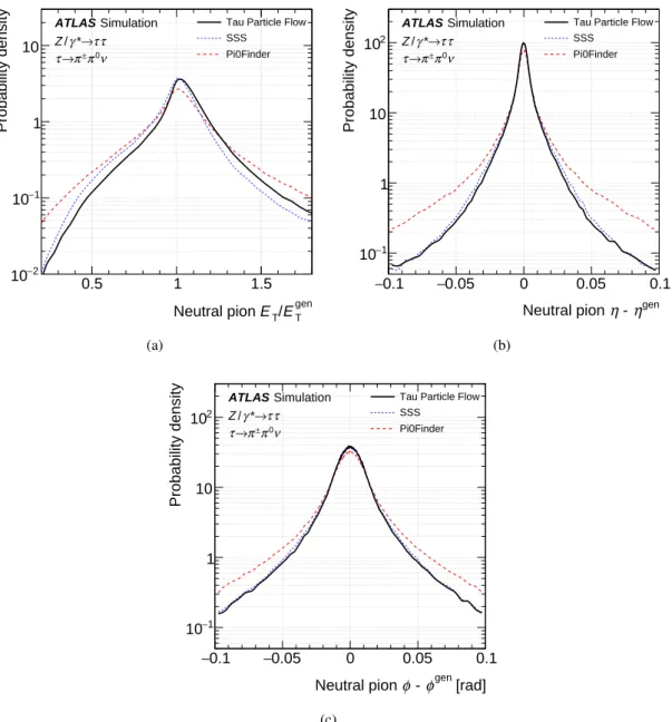
The π0ET, η and φ residual distributions for all π0reconstruction algorithms are shown in Figs.3(a),3(b) and3(c), respectively. The core angular resolutions for each algorithm are quite similar with ∼0.0056 in η and ∼0.012 rad in φ. The Pi0Finder algorithm has the poorest performance, with core resolutions of 0.0086 and 0.016 rad in η and φ, respectively, and significantly larger tails. The core ET resolutions are almost identical for the Tau Particle Flow and SSS, both with 16%, compared to 23% for Pi0Finder. The Tau Particle Flow and SSS both show a shift in the reconstructed ETof a few percent, due to incom-plete subtraction of the h±remnant. In the calculation of the τhad−visfour-momentum in the Tau Particle Flow (Section3.5), this bias is corrected for by a decay-mode-dependent calibration. Despite the more sophisticated shower subtraction employed in the SSS algorithm, it does not perform significantly better; the improvement in the total fraction of correctly classified tau decays is ∼1%. This is partly because many of the π0cand’s are sufficiently displaced from h±’s so that they have little energy contamination and are unaffected by the subtraction, and partly because the signature of clusters that contain π0’s, even in the presence of overlapping h± energy, is distinct enough for the BDT to identify. Contributions from pile-up have little effect on the π0
candreconstruction in Tau Particle Flow; on average the ET increases by ∼15 MeV and its resolution degrades fractionally by ∼0.5% per additional reconstructed vertex.
3.3 Reconstruction of individual photon energy deposits in EM1
During the π0reconstruction, the energy deposits from both photons typically merge into a single cluster. Furthermore, for Z → ττ events, in about half of the h±≥2π0 decays misclassified as h±π0 by the π0 reconstruction, at least three of the photons from two π0’s are grouped into a single cluster. The fraction increases for higher τhad−vispTdue to the collimation of the tau decay products. The identification of the energy deposits from individual photons in the finely segmented EM1 layer can be exploited to improve the π0reconstruction, as discussed in the following.
Almost all photons begin to shower by the time they traverse EM1, where they deposit on average ∼30% of their energy. In contrast, particles that do not interact electromagnetically rarely deposit a significant amount of energy in this layer, making it ideal for the identification of photons. Furthermore, the cell segmentation in η in this layer is finer than the average photon separation and comparable to the average photon shower width, allowing individual photons to be distinguished.
The reconstruction of energy deposits in EM1 proceeds as follows. First, local energy maxima are searched for within the core region. A local maximum is defined as a single cell with ET > 100 MeV whose nearest neighbours in η both have lower ET. Maxima found in adjacent φ cells are then combined:
gen T E / T E Neutral pion 0.5 1 1.5 Probability density 2 − 10 1 − 10 1 10 ATLAS Simulation τ τ → * γ / Z ν 0 π ± π → τ
Tau Particle Flow SSS Pi0Finder (a) gen η - η Neutral pion 0.1 − −0.05 0 0.05 0.1 Probability density 1 − 10 1 10 2 10 ATLAS Simulation τ τ → * γ / Z ν 0 π ± π → τ
Tau Particle Flow SSS Pi0Finder (b) [rad] gen φ - φ Neutral pion 0.1 − −0.05 0 0.05 0.1 Probability density 1 − 10 1 10 2 10 ATLAS Simulation τ τ → * γ / Z ν 0 π ± π → τ
Tau Particle Flow SSS
Pi0Finder
(c)
Figure 3: Distributions of the π0 residuals in (a) transverse energy E
T, (b) pseudorapidity η and (c) azimuth φ in
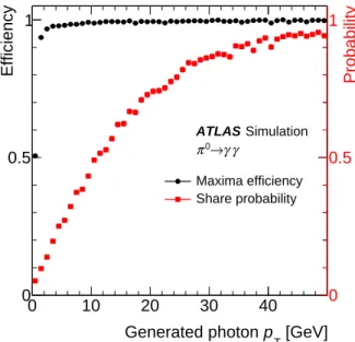
their energy is summed and the energy-weighted mean of their φ positions is used. Figure4shows the efficiency for photons to create a local maximum (maxima efficiency), evaluated in the sample of single π0’s. The efficiency decreases rapidly at low photon p
Tas many of the photons fall below the 100 MeV threshold. The fraction of misreconstructed maxima due to noise or fluctuations from the photon shower is very low for maxima with ET > 500 MeV, but increases quickly at lower ET. At high photon pT, corresponding to high π0 pT, the boost of the π0 becomes large enough that the pair of photons almost always creates a single maximum. Figure4also shows the probability that a maximum is shared with the other photon in the single π0sample (share probability).
[GeV] T p Generated photon 0 10 20 30 40 Efficiency 0 0.5 1 Probability 0 0.5 1 ATLAS Simulation γ γ → 0 π Maxima efficiency Share probability
Figure 4: Efficiency for a photon to create a maximum in the first layer of the EM calorimeter in simulated π0→γγ
events and the corresponding probability to create a maximum that is shared with the other photon. The photons are required to not interact with the material in the tracking system.
The h±≥2π0 decay mode classification is improved by counting the number of maxima associated with π0
cand’s. An energy maximum is assigned to a π 0
candif its cell is part of the π 0
candcluster and it has an ET of more than 300–430 MeV (depending on the η region). The energy threshold is optimised to maximise the total number of correctly classified tau decays. Maxima with ET> 10 GeV are counted twice, as they contain the merged energy deposits of two photons from a π0decay with a probability larger than 95%. Finally, τhad−vis candidates that were classified as h±π0, but have a π0cand with at least three associated maxima are reclassified as h±≥2π0. The method recovers 16% of misclassified h±≥2π0 decays with a misclassification of h±π0decays of 2.5%.
3.4 Decay mode classification
Determination of the decay mode by counting the number of reconstructed h±’s and π0ID’s alone can be significantly improved by simultaneously analysing the kinematics of the tau decay products, the π0 identification scores and the number of photons from the previous reconstruction steps. Exploitation of this information is performed via BDTs.
As the most difficult aspect of the classification is to determine the number of π0’s, three decay mode tests are defined to distinguish between the following decay modes: h±’s with zero or one π0, h±{0, 1}π0; h±’s with one or more π0’s, h±{1, ≥2}π0; and 3h±’s with and without π0’s, 3h±{0, ≥1}π0. Which of the three tests to apply to a τhad−vis candidate is determined as follows. The τhad−vis candidates with one or three associated tracks without any reconstructed π0cand’s are always classified as h±or 3h±, respectively. The τhad−vis candidates with one associated track and at least two π0cand’s, of which at least one is π0ID, enter the h±{1, ≥2}π0test. The τhad−viscandidates with one π0IDthat are classified as h±≥2π0by counting the photons in this cluster, as described in Section3.3, retain their classification and are not considered in the decay mode tests. The remaining τhad−viscandidates with one or three associated tracks enter the h±{0, 1}π0or 3h±{0, ≥1}π0tests, respectively.
A BDT is trained for each decay mode test using τhad−vis candidates from simulated Z → ττ events, to separate τhad−vis’s of the two generated decay types the test is designed to distinguish. The τhad−vis candidates entering each decay mode test are then further categorised based on the number of π0ID’s. A threshold is placed on the output BDT score in each category to determine the decay mode. The thresholds are optimised to maximise the number of correctly classified τhad−vis candidates. The BDT training was not split based on the number of π0ID’s due to the limited size of the training sample.
The variables used for the decay mode tests are designed to discriminate against additional misidentified π0
cand’s, which usually come from imperfect h
±subtraction, pile-up or the underlying event. The associ-ated clusters typically have low energy and a low π0identification score. Remnant clusters from imperfect h±subtraction are also typically close to the h±track and have fewer associated photon energy maxima. If the π0candclusters originate from tau decays, their directions and fractional energies are correlated with each other. Additionally, with increasing number of tau decay products, the available phase space per decay product becomes smaller. Each variable used in the BDTs is described briefly in Table4. Table5 summarises the decay mode tests and indicates which variables are used in each.
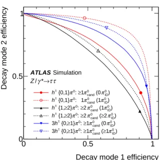
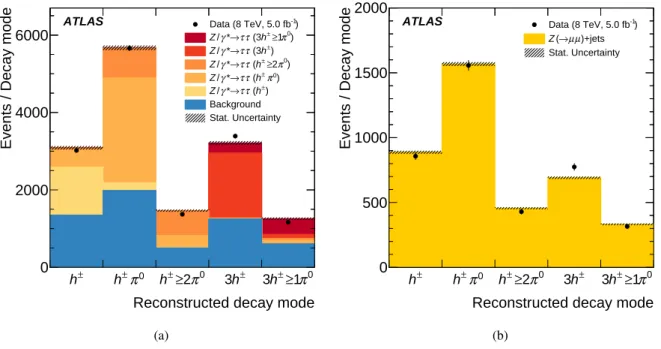
Figure5shows the discrimination power of the tests categorised by the number of π0cand’s and π0ID’s. The decay mode fractions at the input of each test vary strongly, which impacts the position of the optimal BDT requirements. The resulting classification matrix is shown in Fig.6. The total fraction of correctly classified tau decays is 74.7%. High efficiencies in the important h±, h±π0and 3h±modes are achieved. The decay mode purity is defined as the fraction of τhad−vis candidates of a given reconstructed mode which originated from a generated τhad−visof the same mode, also calculated using τhad−vis’s in simulated Z →ττ events. The purity of the h±, h±π0and 3h±decay modes is 70.3%, 73.5% and 85.2%, respectively. For comparison, in the Baseline reconstruction where π0reconstruction was not available, the fractions of generated h±and h±π0in τhad−vis’s with one reconstructed track are 27.4% and 52.2%, respectively, and the fraction of 3h±in τhad−vis’s with three reconstructed tracks is 68.9%. Decays containing neutral kaons are omitted from the table. They are classified as containing π0’s approximately half of the time. Contributions from pile-up have little effect on the classification efficiency, degrading it by ∼0.04% per additional reconstructed vertex. The number of τhad−vis candidates for each classified decay mode is shown in Fig.7(a) for real τhad−vis’s from the Z → ττ tag-and-probe analysis and in Fig. 7(b)for jets from the Z(→ µµ)+jets tag-and-probe analysis. While systematic uncertainties have not been evaluated, the figures indicate reasonable modelling of the decay mode classification for τhad−vis’s and jets. In both selections, the 3h± efficiency is slightly underestimated and the h±≥2π0 and 3h±≥1π0 efficiencies are slightly overestimated.
π0identification score of the firstπ0 cand, S
BDT 1 π0identification score of the π0
candwith the highest π
0identification score ETfraction of the firstπ0cand, fπ0,1
ETof the π0candwith the highest π0identification score, divided by the ET-sum of all π0
cand’s and h ±’s
Hadron separation,∆R(h±, π0) ∆R between the h±and the π0
candwith the highest π
0identification score h±distance, Dh±
ET-weighted∆R between the h± and the τhad−visaxis, which is calculated by sum-ming the four-vectors of all h±’s and π0cand’s
Number of photons, Nγ
Total number of photons in the τhad−vis, as reconstructed in Section3.3 π0identification score of secondπ0
cand, S BDT 2 π0identification score of the π0
candwith the second-highest π
0identification score π0
candETfraction, fπ0
ET-sum of π0cand’s, divided by the ET-sum of π0cand’s and h±’s π0
candmass, mπ0
Invariant mass calculated from the sum of π0candfour-vectors Number ofπ0
cand, Nπ0
Standard deviation of the h± pT,σET,h±
Standard deviation, calculated from the pT values of the h±’s for τhad−viswith three associated tracks
h±mass, mh±
Invariant mass calculated from the sum of h±four-vectors
Table 4: Variables used in the BDTs for the τhad−vis decay mode classification. They are designed to discriminate
against additional misidentified π0
cand’s, which usually come from imperfect subtraction, pile-up or the underlying
Decay mode test N(π0cand) N(π0ID) Variables h±{0, 1}π0 ≥ 1 0 SBDT1 , fπ0,1,∆R(h±, π0), Dh±, Nγ 1 1 h±{1, ≥2}π0 ≥ 2 1 SBDT2 , fπ0, mπ0, Nπ0, Nγ ≥ 2 ≥ 2 3h±{0, ≥1}π0 ≥ 1≥ 1 ≥ 10 SBDT1 , fπ0, σET,h±, mh±, Nγ
Table 5: Details regarding the decay mode classification of the Tau Particle Flow. BDTs are trained to distinguish decay modes in three decay mode tests. The τhad−vis’s entering each test are further categorised based on the number
of reconstructed, N(π0
cand), and identified, N(π 0
ID), neutral pions. The variables used in the BDTs for each test are
listed.
Decay mode 1 efficiency
0 0.5 1
Decay mode 2 efficiency
0 0.5 1 ATLAS Simulation τ τ → * γ / Z ) ID 0 π (0 cand 0 π 1 ≥ : 0 π {0,1} ± h ) ID 0 π (1 cand 0 π : 1 0 π {0,1} ± h ) ID 0 π (1 cand 0 π 2 ≥ : 0 π 2} ≥ {1, ± h ) ID 0 π 2 ≥ ( cand 0 π 2 ≥ : 0 π 2} ≥ {1, ± h ) ID 0 π (0 cand 0 π 1 ≥ : 0 π 1} ≥ {0, ± h 3 ) ID 0 π 1 ≥ ( cand 0 π 1 ≥ : 0 π 1} ≥ {0, ± h 3
Figure 5: Decay mode classification efficiency for the h±{0, 1}π0, h±{1, ≥2}π0, and 3h±{0, ≥1}π0 tests. For each test, “decay mode 1” corresponds to the mode with fewer π0’s. Working points corresponding to the optimal thresholds on the BDT score for each test are marked.
89.7 16.0 4.3 1.2 0.3
9.4 74.8 56.3 0.9 2.5
0.4 6.0 35.4 0.1 0.4
0.2 0.6 0.3 92.5 40.2
0.2 2.5 3.6 5.3 56.6
Generated decay mode ± h h±π0 π0 2 ≥ ± h 3h± π0 1 ≥ ± h 3
Reconstructed decay mode
± h 0 π ± h 0 π 2 ≥ ± h ± h 3 0 π 1 ≥ ± h 3 ATLAS Simulation
Tau Particle Flow
τ τ → * γ / Z Diagonal fraction: 74.7%
Figure 6: Decay mode classification efficiency matrix showing the probability for a given generated mode to be reconstructed as a particular mode by the Tau Particle Flow after final decay mode classification in simulated Z → ττ events. Decays containing neutral kaons are omitted. Only decays from τhad−vis’s that are reconstructed
and pass the selection described in Section2.2are considered. The statistical uncertainty is negligible.
Reconstructed decay mode
±
h h±π0 h±≥2π0 3h± 3h±≥1π0
Events / Decay mode
0 2000 4000 6000
ATLAS Data (8 TeV, 5.0 fb-1) ) 0 π 1 ≥ ± h (3 τ τ → * γ / Z ) ± h (3 τ τ → * γ / Z ) 0 π 2 ≥ ± h ( τ τ → * γ / Z ) 0 π ± h ( τ τ → * γ / Z ) ± h ( τ τ → * γ / Z Background Stat. Uncertainty (a)
Reconstructed decay mode
±
h h±π0 h±≥2π0 3h± 3h±≥1π0
Events / Decay mode
0 500 1000 1500 2000
ATLAS Data (8 TeV, 5.0 fb-1) )+jets µ µ → ( Z Stat. Uncertainty (b)
Figure 7: Number of τhad−viscandidates for each classified decay mode in the (a) Z → ττ and the (b) Z(→ µµ)+jets
tag-and-probe analyses. The simulated Z → ττ sample is split into contributions from each generated tau decay mode. The background in the Z → ττ analysis is dominated by multijet and W(→ µν)+jets production. The simulated Z(→ µµ)+jets events are reweighted so that the Z boson pT distribution and the overall normalisation
3.5 Four-momentum reconstruction
The τhad−vis four-momentum reconstruction begins with summing the four-momenta of the h±and π0cand constituents (Constituent-based calculation). Only the first n π0cand’s with the highest π0 identification scores are included, where n is determined from the decay mode classification, and can be at most 2 π0cand’s in the h±≥2π0 mode and at most 1 π0cand in the 3h±≥1π0 mode. A pion mass hypothesis is used for π0
cand’s. There are two exceptions: if the decay mode is classified as h
±π0 but there are two identified π0
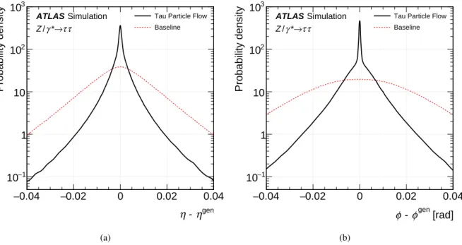
cand’s, the mass of each is set to zero and both are added to the τhad−visfour-momentum as they are most likely photons from a π0decay; or if the τhad−viscandidate is classified as h±≥2π0because three or more photons are found in a single π0cand, only this π0candis added and its mass is set to twice the π0mass. A calibration is applied to the Constituent-based τhad−vis energy in each decay mode as a function of the Constituent-based ET, to correct for the π0candenergy bias. The resulting four-momentum is used to set the τhad−vis direction in the Tau Particle Flow. Figures 8(a) and8(b) show distributions of the τhad−vis η and φ residuals of the Tau Particle Flow and the Baseline four-momentum reconstruction. The core angular resolutions of the Tau Particle Flow are 0.002 in η and 0.004 rad in φ, which are more than five times better than the Baseline resolutions of 0.012 and 0.02 rad, respectively.
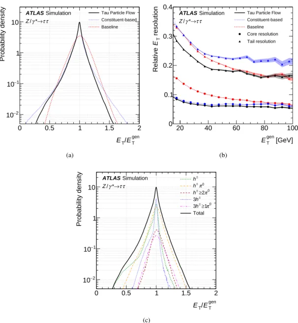
Figure9(a)shows distributions of the ETresiduals. The Constituent-based calculation is inherently stable against pile-up as both the decay-mode classification used to select h±’s and π0cand’s, and the reconstruction of h±’s and π0cand’s themselves, are stable against pile-up. The ETincreases by ∼6 MeV and its resolution degrades fractionally by ∼0.6% per additional reconstructed vertex. Figure9(b)shows the resolution as a function of the ET of the generated τhad−vis. For the final energy calibration of the Tau Particle Flow, the Constituent-based ET is combined with the Baseline ET by weighting each by the inverse-square of their respective ET-dependent core resolutions, which ensures a smooth transition to high pT where the Baseline calibration is superior. The Baseline ET is used if the two ET values disagree by more than five times their combined core resolutions, as it has smaller resolution tails. The resolution of the Tau Particle Flow is superior in both the core and tails at low ET with a core resolution of 8% at an ET of 20 GeV, compared to 15% from the Baseline. It approaches the Baseline performance at high ET. Contributions from pile-up have little effect on the four-momentum reconstruction of the Tau Particle Flow; the ETincreases by ∼4 MeV and its core resolution degrades fractionally by ∼0.5% per additional reconstructed vertex. The ET residual distributions of the Tau Particle Flow split into the reconstructed decay modes are shown in Fig. 9(c). The total is non-Gaussian, as it is the sum of contributions with different functional forms. Correctly reconstructed decays containing only h±
’s have the best resolution, followed by correctly reconstructed decays containing π0cand’s. The excellent resolution of these decays leads to a superior overall core resolution. Misreconstructed decays have the poorest resolution and result in larger tails. In particular, misestimation of the number of π0cand’s leads to a bias of up to 25%. Decays containing neutral kaons exhibit a large low-energy bias because at least some of their energy is typically missed by the reconstruction.
An alternative method for the ETcalibration was also developed, based on Ref. [30]. It also uses a com-bination of calorimetric and tracking measurements and the Tau Particle Flow decay mode classification. The h± pT is measured using tracks and the π0 ET is estimated as the difference between the ET of the seed jet at the EM scale [36] and the ET from the summed momenta of all h±’s, scaled by their expected calorimeter response [60]. The method has similar overall performance to the Tau Particle Flow.
cal-gen η - η 0.04 − −0.02 0 0.02 0.04 Probability density 1 − 10 1 10 2 10 3 10 ATLAS Simulation τ τ → * γ / Z
Tau Particle Flow Baseline (a) [rad] gen φ - φ 0.04 − −0.02 0 0.02 0.04 Probability density 1 − 10 1 10 2 10 3 10 ATLAS Simulation τ τ → * γ / Z
Tau Particle Flow Baseline
(b)
Figure 8: The τhad−vis (a) η and (b) φ residual distributions of the Tau Particle Flow compared to the Baseline
reconstruction.
the τhad−visETand analysis of the distribution has previously been used to calibrate the τhad−visET[17]. Data and simulation agree well, indicating that the τhad−visETis well modelled by the simulation. Finally,
Fig.10(b)shows the mass spectrum of the τhad−visreconstructed with the Tau Particle Flow in the Z → ττ
tag-and-probe analysis. The a1 resonance in the 3h±mode is reconstructed with negligible experimental resolution compared to the intrinsic line shape due to the excellent four-momentum resolution of the in-ner detector for h±’s. The ρ and a1resonances in the h±π0and h±≥2π0modes are also visible, but have significant degradation due to the resolution from the reconstructed π0candfour-momentum. The τhad−vis mass spectra in data and simulation agree well, suggesting good modelling of the individual h±and π0cand four-momenta.
gen T E / T E 0 0.5 1 1.5 2 Probability density 2 − 10 1 − 10 1 10 ATLAS Simulation τ τ → * γ / Z
Tau Particle Flow Constituent-based Baseline (a) [GeV] gen T E 20 40 60 80 100 resolutionT E Relative 0 0.1 0.2 0.3 0.4 τ τ → * γ / Z
ATLAS Simulation Tau Particle Flow
Constituent-based Baseline Core resolution Tail resolution (b) gen T E / T E 0 0.5 1 1.5 2 Probability density 2 − 10 1 − 10 1 10 ATLAS Simulation τ τ → * γ / Z ± h 0 π ± h 0 π 2 ≥ ± h ± h 3 0 π 1 ≥ ± h 3 Total (c)
Figure 9: The (a) τhad−vis relative ET residual distribution and (b) the half-widths spanned by the 68% and 95%
quantiles, i.e. the core and tail resolutions, of the relative ET residual distributions as a function of the generated
τhad−visET. The Baseline, Constituent-based and Tau Particle Flow calculations are shown. The relative ETresidual
Events / 5 GeV 0 500 1000 1500 2000 2500 3000 3500
ATLAS Data (8 TeV, 5.0 fb-1) ) 0 π 1 ≥ ± h (3 τ τ → * γ / Z ) ± h (3 τ τ → * γ / Z ) 0 π 2 ≥ ± h ( τ τ → * γ / Z ) 0 π ± h ( τ τ → * γ / Z ) ± h ( τ τ → * γ / Z Background Stat. Uncertainty ) [GeV] had-vis τ , µ ( m 50 100 150 Obs. / exp. 0.5 1 1.5 (a) Events / 0.1 GeV 0 500 1000 1500 2000 2500 3000 3500
ATLAS Data (8 TeV, 5.0 fb-1) ) 0 π 1 ≥ ± h (3 τ τ → * γ / Z ) ± h (3 τ τ → * γ / Z ) 0 π 2 ≥ ± h ( τ τ → * γ / Z ) 0 π ± h ( τ τ → * γ / Z ) ± h ( τ τ → * γ / Z Background Stat. Uncertainty mass [GeV] had-vis τ Reconstructed 0 0.5 1 1.5 2 Obs. / exp. 0.5 1 1.5 (b)
Figure 10: Distribution of (a) the invariant mass of the muon and τhad−vis, m(µ, τhad−vis) before selection on
m(µ, τhad−vis) is applied; and (b) the reconstructed mass of the τhad−vis, when using the Tau Particle Flow τhad−vis
four-momentum reconstruction in the Z → ττ tag-and-probe analysis. The simulated Z → ττ sample is split into contributions from each generated tau decay mode. The background is dominated by multijet and W(→ µν)+jets production. The hatched band represents the statistical uncertainty on the prediction.
4 Summary and conclusions
This paper presents a new method to reconstruct the individual charged and neutral hadrons in tau decays with the ATLAS detector at the LHC. The neutral pions are reconstructed with a core energy resolution of ∼16%. The reconstructed hadrons are used to calculate the visible four-momentum of reconstructed tau candidates and to classify the decay mode, allowing the decays to be distinguished not only by the number of h±’s but also by the number of π0’s, which is not possible with the existing tau reconstruction. This improves the purity with which the τ− → π−ν, τ− → π−π0ν and τ− → π−π+π−ν decays can be selected, by factors of 2.6, 1.4 and 1.2, respectively. The τhad−viscore directional resolution is improved by more than a factor of five and the core energy resolution is improved by up to a factor of two at low ET (20 GeV). The performance was validated using samples of Z → ττ and Z(→ µµ)+jets events selected from pp collision data at √s= 8 TeV, corresponding to an integrated luminosity of 5 fb−1. The results suggest good modelling of the τhad−visdecay mode classification efficiency and four-momentum reconstruction.
Acknowledgements
We thank CERN for the very successful operation of the LHC, as well as the support staff from our institutions without whom ATLAS could not be operated efficiently.
We acknowledge the support of ANPCyT, Argentina; YerPhI, Armenia; ARC, Australia; BMWFW and FWF, Austria; ANAS, Azerbaijan; SSTC, Belarus; CNPq and FAPESP, Brazil; NSERC, NRC and CFI, Canada; CERN; CONICYT, Chile; CAS, MOST and NSFC, China; COLCIENCIAS, Colombia; MSMT CR, MPO CR and VSC CR, Czech Republic; DNRF and DNSRC, Denmark; IN2P3-CNRS, CEA-DSM/IRFU, France; GNSF, Georgia; BMBF, HGF, and MPG, Germany; GSRT, Greece; RGC, Hong Kong SAR, China; ISF, I-CORE and Benoziyo Center, Israel; INFN, Italy; MEXT and JSPS, Japan; CNRST, Morocco; FOM and NWO, Netherlands; RCN, Norway; MNiSW and NCN, Poland; FCT, Por-tugal; MNE/IFA, Romania; MES of Russia and NRC KI, Russian Federation; JINR; MESTD, Serbia; MSSR, Slovakia; ARRS and MIZŠ, Slovenia; DST/NRF, South Africa; MINECO, Spain; SRC and Wallenberg Foundation, Sweden; SERI, SNSF and Cantons of Bern and Geneva, Switzerland; MOST, Taiwan; TAEK, Turkey; STFC, United Kingdom; DOE and NSF, United States of America. In addition, individual groups and members have received support from BCKDF, the Canada Council, CANARIE, CRC, Compute Canada, FQRNT, and the Ontario Innovation Trust, Canada; EPLANET, ERC, FP7, Ho-rizon 2020 and Marie Skłodowska-Curie Actions, European Union; Investissements d’Avenir Labex and Idex, ANR, Région Auvergne and Fondation Partager le Savoir, France; DFG and AvH Foundation, Ger-many; Herakleitos, Thales and Aristeia programmes co-financed by EU-ESF and the Greek NSRF; BSF, GIF and Minerva, Israel; BRF, Norway; the Royal Society and Leverhulme Trust, United Kingdom. The crucial computing support from all WLCG partners is acknowledged gratefully, in particular from CERN and the ATLAS Tier-1 facilities at TRIUMF (Canada), NDGF (Denmark, Norway, Sweden), CC-IN2P3 (France), KIT/GridKA (Germany), INFN-CNAF (Italy), NL-T1 (Netherlands), PIC (Spain), ASGC (Taiwan), RAL (UK) and BNL (USA) and in the Tier-2 facilities worldwide.
References
[1] ATLAS Collaboration, The ATLAS Experiment at the CERN Large Hadron Collider,
JINST 3 (2008) S08003.
[2] L. Evans and P. Bryant, LHC Machine,JINST 3 (2008) S08001. [3] ATLAS Collaboration,
Measurement of the t¯t production cross section in the tau+jets channel using the ATLAS detector,
Eur. Phys. J. C 73 (2013) 2328, arXiv:1211.7205 [hep-ex].
[4] ATLAS Collaboration,
Measurement of the top quark pair cross section with ATLAS in pp collisions at √s= 7 TeV using final states with an electron or a muon and a hadronically decayingτ lepton,
Phys. Lett. B 717 (2012) 89, arXiv:1205.2067 [hep-ex].
[5] ATLAS Collaboration, Measurement of the W → τντcross section in pp collisions at √s= 7 TeV with the ATLAS experiment,Phys. Lett. B 706 (2012) 276, arXiv:1108.4101 [hep-ex].
[6] ATLAS Collaboration, Measurement of τ polarization in W → τν decays with the ATLAS detector in pp collisions at √s= 7 TeV,Eur. Phys. J. C 72 (2012) 2062, arXiv:1204.6720 [hep-ex]. [7] ATLAS Collaboration, Measurement of the Z → ττ cross section with the ATLAS detector,
[9] ATLAS Collaboration, Search for charged Higgs bosons through the violation of lepton universality in t¯t events using pp collision data at √s= 7 TeV with the ATLAS experiment,
JHEP 1303 (2013) 076, arXiv:1212.3572 [hep-ex].
[10] ATLAS Collaboration, Search for charged Higgs bosons decaying via H±→τν in t¯t events using pp collision data at √s= 7 TeV with the ATLAS detector,JHEP 1206 (2012) 039,
arXiv:1204.2760 [hep-ex].
[11] ATLAS Collaboration, Search for the neutral Higgs bosons of the Minimal Supersymmetric Standard Model in pp collisions at √s= 7 TeV with the ATLAS detector,JHEP 1302 (2013) 095, arXiv:1211.6956 [hep-ex].
[12] ATLAS Collaboration,
Search for supersymmetry in events with large missing transverse momentum, jets, and at least one tau lepton in20 fb−1of √s= 8 TeV proton–proton collision data with the ATLAS detector,
JHEP 1409 (2014) 103, arXiv:1407.0603 [hep-ex].
[13] ATLAS Collaboration, Search for the direct production of charginos, neutralinos and staus in final states with at least two hadronically decaying taus and missing transverse momentum in pp collisions at √s= 8 TeV with the ATLAS detector,JHEP 1410 (2014) 096,
arXiv:1407.0350 [hep-ex].
[14] ATLAS Collaboration, Search for a heavy narrow resonance decaying to eµ, eτ, or µτ with the ATLAS detector in √s= 7 TeV pp collisions at the LHC,Phys. Lett. B 723 (2013) 15,
arXiv:1212.1272 [hep-ex].
[15] ATLAS Collaboration, A search for high-mass resonances decaying to τ+τ−in pp collisions at √
s= 7 TeV with the ATLAS detector,Phys. Lett. B 719 (2013) 242, arXiv:1210.6604 [hep-ex]. [16] ATLAS Collaboration, Search for third generation scalar leptoquarks in pp collisions at
√
s= 7 TeV with the ATLAS detector,JHEP 1306 (2013) 033, arXiv:1303.0526 [hep-ex]. [17] ATLAS Collaboration, Identification and energy calibration of hadronically decaying tau leptons
with the ATLAS experiment in pp collisions at √s= 8 TeV,Eur. Phys. J. C 75 (2015) 303, arXiv:1412.7086 [hep-ex].
[18] ATLAS Collaboration, Observation of a new particle in the search for the Standard Model Higgs boson with the ATLAS detector at the LHC,Phys. Lett. B 716 (2012) 1,
arXiv:1207.7214 [hep-ex]. [19] CMS Collaboration,
Observation of a new boson at a mass of 125 GeV with the CMS experiment at the LHC,
Phys. Lett. B 716 (2012) 30, arXiv:1207.7235 [hep-ex].
[20] CMS Collaboration, Evidence for the 125 GeV Higgs boson decaying to a pair of τ leptons,
JHEP 1405 (2014) 104, arXiv:1401.5041 [hep-ex].
[21] K. Desch et al., Probing the CP nature of the Higgs boson at linear colliders with tau spin correlations: The Case of mixed scalar - pseudoscalar couplings,Phys. Lett. B 579 (2004) 157, arXiv:hep-ph/0307331 [hep-ph].
[22] R. Harnik et al., Measuring CP violation in h → τ+τ−at colliders,
Phys. Rev. D 88 (2013) 076009, arXiv:1308.1094 [hep-ph].
[23] S. Berge, W. Bernreuther and S. Kirchner,
Prospects of constraining the Higgs boson’s CP nature in the tau decay channel at the LHC,
[24] A. Elagin et al., A New Mass Reconstruction Technique for Resonances Decaying to di-tau,
Nucl. Instrum. Meth. A 654 (2011) 481, arXiv:1012.4686 [hep-ex].
[25] ALEPH Collaboration, S. Schael et al., Branching ratios and spectral functions of tau decays: Final ALEPH measurements and physics implications,Phys. Rept. 421 (2005) 191,
arXiv:hep-ex/0506072 [hep-ex]. [26] OPAL Collaboration, R. Akers et al.,
Measurement of theτ−→ h−π0ντandτ−→ h−≥ 2π0ντbranching ratios,
Phys. Lett. B 328 (1994) 207.
[27] DELPHI Collaboration, J. Abdallah et al., A Measurement of the tau hadronic branching ratios,
Eur. Phys. J. C 46 (2006) 1, arXiv:hep-ex/0603044 [hep-ex].
[28] L3 Collaboration, M. Acciarri et al., Measurement of tau polarization at LEP,
Phys. Lett. B 429 (1998) 387.
[29] A. Elagin et al., Probabilistic Particle Flow Algorithm for High Occupancy Environment,
Nucl. Instrum. Meth. A705 (2013) 93–105, arXiv:1207.4780 [hep-ex].
[30] D0 Collaboration, V.M. Abazov et al.,
Measurement ofσ(p ¯p → Z + X) Br(Z → τ+τ−) at √s= 1.96 TeV,Phys. Lett. B 670 (2009) 292, arXiv:0808.1306 [hep-ex].
[31] CMS Collaboration,
Reconstruction and identification ofτ lepton decays to hadrons and ντat CMS,
JINST 11 (2016) P01019, arXiv:1510.07488 [physics.ins-det].
[32] ATLAS Collaboration, Performance of the ATLAS Trigger System in 2010,
Eur. Phys. J. C 72 (2012) 1849, arXiv:1110.1530 [hep-ex].
[33] M. Cacciari, G. P. Salam and G. Soyez, The anti-ktjet clustering algorithm,
JHEP 0804 (2008) 063, arXiv:0802.1189 [hep-ph].
[34] M. Cacciari and G. P. Salam, Dispelling the N3myth for the ktjet-finder,
Phys. Lett. B 641 (2006) 57, eprint:hep-ph/0512210.
[35] W. Lampl et al., Calorimeter Clustering Algorithms: Description and Performance, ATL-LARG-PUB-2008-002, 2008, url:http://cds.cern.ch/record/1099735. [36] T. Barillari et al., Local hadronic calibration, ATL-LARG-PUB-2009-001, 2009,
url:http://cds.cern.ch/record/1112035.
[37] A. Hoecker et al., TMVA: Toolkit for Multivariate Data Analysis, PoS ACAT (2007) 040, arXiv:physics/0703039.
[38] ATLAS Collaboration, Measurement of the muon reconstruction performance of the ATLAS detector using 2011 and 2012 LHC proton–proton collision data,Eur. Phys. J. C 74 (2014) 3130, arXiv:1407.3935 [hep-ex].
[39] ATLAS Collaboration, Performance of missing transverse momentum reconstruction in proton–proton collisions at √s= 7 TeV with ATLAS,Eur. Phys. J. C 72 (2012) 1844, arXiv:1108.5602 [hep-ex].
[42] P. Golonka and Z. Was,
PHOTOS Monte Carlo: a precision tool for QED corrections in Z and W decays,
Eur. Phys. J. C 45 (2006) 97–107, arXiv:hep-ph/0506026.
[43] T. Sjöstrand, S. Mrenna and P. Skands, A brief introduction to PYTHIA 8.1,
Comput. Phys. Commun. 178 (2008) 852–867, arXiv:0710.3820 [hep-ph].
[44] P. M. Nadolsky et al., Implications of CTEQ global analysis for collider observables,
Phys. Rev. D 78, 013004 (2008) 013004, arXiv:0802.0007 [hep-ph].
[45] ATLAS Collaboration, Summary of ATLAS Pythia 8 tunes, ATL-PHYS-PUB-2012-003, 2012,
url:http://cds.cern.ch/record/1474107.
[46] M. L. Mangano et al.,
ALPGEN, a generator for hard multiparton processes in hadronic collisions,
JHEP 0307 (2003) 001, arXiv:hep-ph/0206293 [hep-ph].
[47] P. Z. Skands, Tuning Monte Carlo Generators: The Perugia Tunes,
Phys. Rev. D 82 (2010) 074018, arXiv:1005.3457 [hep-ph].
[48] S. Frixione and B. R. Webber, Matching NLO QCD computations and parton shower simulations,
JHEP 0206 (2002) 29, arXiv:hep-ph/0204244.
[49] S. Frixione et al., Single-top production in MC@NLO,JHEP 0603 (2006) 92, arXiv:hep-ph/0512250.
[50] S. Frixione et al., Single-top hadroproduction in association with a W boson,
JHEP 0807 (2008) 29, arXiv:0805.3067 [hep-ph].
[51] G. Corcella et al., HERWIG 6: an event generator for hadron emission reactions with interfering gluons (including supersymmetric processes),JHEP 0101 (2001) 10, arXiv:hep-ph/0011363. [52] J. M. Butterworth, J. R. Forshaw and M. H. Seymour,
Multiparton interactions in photoproduction at HERA,Z. Phys. C 72 (1996) 637–646, eprint:hep-ph/9601371.
[53] H.-L. Lai et al., New parton distributions for collider physics,
Phys. Rev. D 82, 074024 (2010) 074024, arXiv:1007.2241 [hep-ph].
[54] ATLAS Collaboration, The ATLAS Simulation Infrastructure,Eur. Phys. J. C 70 (2010) 823, arXiv:1005.4568 [hep-ex].
[55] GEANT4 Collaboration, S. Agostinelli et al., Geant4 – a simulation toolkit,
Nucl. Instr. and Meth. A 506 (2003) 250 –303.
[56] G. Folger and J. P. Wellisch, String parton models in Geant4, (2003), arXiv:nucl-th/0306007. [57] H. W. Bertini,
Intranuclear-cascade calculation of the secondary nucleon spectra from nucleon-nucleus interactions in the energy range 340 to 2900 MeV and comparisons with experiment,
Phys. Rev. 188 (1969) 1711.
[58] ATLAS Collaboration, Measurement of the production cross section of jets in association with a Z boson in pp collisions at √s= 7 TeV with the ATLAS detector,JHEP 1307 (2013) 032, arXiv:1304.7098 [hep-ex].
[60] ATLAS Collaboration,
A measurement of single hadron response using data at √s= 8 TeV with the ATLAS detector, ATL-PHYS-PUB-2014-002, 2014, url:http://cdsweb.cern.ch/record/1668961.
The ATLAS Collaboration
G. Aad85, B. Abbott113, J. Abdallah151, O. Abdinov11, R. Aben107, M. Abolins90, O.S. AbouZeid158, H. Abramowicz153, H. Abreu152, R. Abreu116, Y. Abulaiti146a,146b, B.S. Acharya164a,164b,a,
L. Adamczyk38a, D.L. Adams25, J. Adelman108, S. Adomeit100, T. Adye131, A.A. Affolder74, T. Agatonovic-Jovin13, J. Agricola54, J.A. Aguilar-Saavedra126a,126f, S.P. Ahlen22, F. Ahmadov65,b, G. Aielli133a,133b, H. Akerstedt146a,146b, T.P.A. Åkesson81, A.V. Akimov96, G.L. Alberghi20a,20b, J. Albert169, S. Albrand55, M.J. Alconada Verzini71, M. Aleksa30, I.N. Aleksandrov65, C. Alexa26b, G. Alexander153, T. Alexopoulos10, M. Alhroob113, G. Alimonti91a, L. Alio85, J. Alison31, S.P. Alkire35, B.M.M. Allbrooke149, P.P. Allport18, A. Aloisio104a,104b, A. Alonso36, F. Alonso71, C. Alpigiani138, A. Altheimer35, B. Alvarez Gonzalez30, D. Álvarez Piqueras167, M.G. Alviggi104a,104b, B.T. Amadio15, K. Amako66, Y. Amaral Coutinho24a, C. Amelung23, D. Amidei89, S.P. Amor Dos Santos126a,126c, A. Amorim126a,126b, S. Amoroso48, N. Amram153, G. Amundsen23, C. Anastopoulos139, L.S. Ancu49, N. Andari108, T. Andeen35, C.F. Anders58b, G. Anders30, J.K. Anders74, K.J. Anderson31,
A. Andreazza91a,91b, V. Andrei58a, S. Angelidakis9, I. Angelozzi107, P. Anger44, A. Angerami35, F. Anghinolfi30, A.V. Anisenkov109,c, N. Anjos12, A. Annovi124a,124b, M. Antonelli47, A. Antonov98, J. Antos144b, F. Anulli132a, M. Aoki66, L. Aperio Bella18, G. Arabidze90, Y. Arai66, J.P. Araque126a, A.T.H. Arce45, F.A. Arduh71, J-F. Arguin95, S. Argyropoulos63, M. Arik19a, A.J. Armbruster30,
O. Arnaez30, H. Arnold48, M. Arratia28, O. Arslan21, A. Artamonov97, G. Artoni23, S. Artz83, S. Asai155, N. Asbah42, A. Ashkenazi153, B. Åsman146a,146b, L. Asquith149, K. Assamagan25, R. Astalos144a,
M. Atkinson165, N.B. Atlay141, K. Augsten128, M. Aurousseau145b, G. Avolio30, B. Axen15,
M.K. Ayoub117, G. Azuelos95,d, M.A. Baak30, A.E. Baas58a, M.J. Baca18, H. Bachacou136, K. Bachas154, M. Backes30, M. Backhaus30, P. Bagiacchi132a,132b, P. Bagnaia132a,132b, Y. Bai33a, T. Bain35,
J.T. Baines131, O.K. Baker176, E.M. Baldin109,c, P. Balek129, T. Balestri148, F. Balli84, W.K. Balunas122, E. Banas39, Sw. Banerjee173,e, A.A.E. Bannoura175, L. Barak30, E.L. Barberio88, D. Barberis50a,50b, M. Barbero85, T. Barillari101, M. Barisonzi164a,164b, T. Barklow143, N. Barlow28, S.L. Barnes84, B.M. Barnett131, R.M. Barnett15, Z. Barnovska5, A. Baroncelli134a, G. Barone23, A.J. Barr120, F. Barreiro82, J. Barreiro Guimarães da Costa33a, R. Bartoldus143, A.E. Barton72, P. Bartos144a,
A. Basalaev123, A. Bassalat117, A. Basye165, R.L. Bates53, S.J. Batista158, J.R. Batley28, M. Battaglia137, M. Bauce132a,132b, F. Bauer136, H.S. Bawa143, f, J.B. Beacham111, M.D. Beattie72, T. Beau80,
P.H. Beauchemin161, R. Beccherle124a,124b, P. Bechtle21, H.P. Beck17,g, K. Becker120, M. Becker83, M. Beckingham170, C. Becot117, A.J. Beddall19b, A. Beddall19b, V.A. Bednyakov65, C.P. Bee148, L.J. Beemster107, T.A. Beermann30, M. Begel25, J.K. Behr120, C. Belanger-Champagne87, W.H. Bell49, G. Bella153, L. Bellagamba20a, A. Bellerive29, M. Bellomo86, K. Belotskiy98, O. Beltramello30,
O. Benary153, D. Benchekroun135a, M. Bender100, K. Bendtz146a,146b, N. Benekos10, Y. Benhammou153, E. Benhar Noccioli49, J.A. Benitez Garcia159b, D.P. Benjamin45, J.R. Bensinger23, S. Bentvelsen107, L. Beresford120, M. Beretta47, D. Berge107, E. Bergeaas Kuutmann166, N. Berger5, F. Berghaus169, J. Beringer15, C. Bernard22, N.R. Bernard86, C. Bernius110, F.U. Bernlochner21, T. Berry77, P. Berta129, C. Bertella83, G. Bertoli146a,146b, F. Bertolucci124a,124b, C. Bertsche113, D. Bertsche113, M.I. Besana91a, G.J. Besjes36, O. Bessidskaia Bylund146a,146b, M. Bessner42, N. Besson136, C. Betancourt48,
S. Bethke101, A.J. Bevan76, W. Bhimji15, R.M. Bianchi125, L. Bianchini23, M. Bianco30, O. Biebel100, D. Biedermann16, N.V. Biesuz124a,124b, M. Biglietti134a, J. Bilbao De Mendizabal49, H. Bilokon47, M. Bindi54, S. Binet117, A. Bingul19b, C. Bini132a,132b, S. Biondi20a,20b, D.M. Bjergaard45,
C.W. Black150, J.E. Black143, K.M. Black22, D. Blackburn138, R.E. Blair6, J.-B. Blanchard136,
J.E. Blanco77, T. Blazek144a, I. Bloch42, C. Blocker23, W. Blum83,∗, U. Blumenschein54, S. Blunier32a, G.J. Bobbink107, V.S. Bobrovnikov109,c, S.S. Bocchetta81, A. Bocci45, C. Bock100, M. Boehler48,
![Table 2: Five dominant τ had−vis decay modes [59]. Tau neutrinos are omitted from the table](https://thumb-eu.123doks.com/thumbv2/123doknet/14098255.465287/6.892.297.623.145.287/table-dominant-decay-modes-tau-neutrinos-omitted-table.webp)