Behavior of Lower Hybrid Waves in the Scrape Off Layer of a Diverted Tokamak

(1)

Plasma Science and Fusion Center Massachusetts Institute of Technology

Cambridge MA 02139 USA

November 2009

This work was supported by the U.S. Department of Energy, Grant No.

DE-FC02-99ER54512. Reproduction, translation, publication, use and disposal, in whole or in part, by or for the United States government is permitted.

PSFC/RR-09-14 DOE/ET-54512-368

Behavior of Lower Hybrid Waves in the Scrape Off

Layer of a Diverted Tokamak

(2)

Behavior of Lower Hybrid Waves in the Scrape Off

Layer of a Diverted Tokamak

by

Gregory M. Wallace

Submitted to the Department of Nuclear Science and Engineering

in partial fulfillment of the requirements for the degree of

Doctor of Philosophy in Applied Plasma Physics

at the

MASSACHUSETTS INSTITUTE OF TECHNOLOGY

February 2010

c

° Massachusetts Institute of Technology 2010. All rights reserved.

Author . . . .

Department of Nuclear Science and Engineering

November 12, 2009

Certified by . . . .

Ronald R. Parker

Professor, Department of Nuclear Science and Engineering

Thesis Supervisor

Certified by . . . .

Dennis G. Whyte

Professor, Department of Nuclear Science and Engineering

Thesis Reader

Certified by . . . .

Paul T. Bonoli

Senior Research Scientist, MIT Plasma Science and Fusion Center

Thesis Reader

Accepted by . . . .

(3)

(4)

Behavior of Lower Hybrid Waves in the Scrape Off Layer of

a Diverted Tokamak

by

Gregory M. Wallace

Submitted to the Department of Nuclear Science and Engineering on November 12, 2009, in partial fulfillment of the

requirements for the degree of

Doctor of Philosophy in Applied Plasma Physics

Abstract

The goal of the Lower Hybrid Current Drive (LHCD) system on the Alcator C-Mod tokamak is to investigate current profile control under plasma conditions relevant to future devices such as ITER and DEMO. This thesis addresses the behavior of Lower Hybrid (LH) waves in the edge and Scrape Off Layer (SOL) of Alcator C-Mod, a compact, high field, high density, diverted tokamak.

The results of coupling experiments over a range of plasma parameters in both L-and H-mode plasmas are presented. Experimental observations suggest that power absorption in the SOL (from both Ion Cyclotron Heating and LHCD sources) modifies the density profile in the vicinity of the LH launcher, thereby affecting the coupling of LH waves.

An analysis of the damage sustained by the LH launcher also shows absorption of the LH waves in the SOL near the antenna. Estimates of the heat flux sustained by the antenna during high power LHCD are in agreement with measurements of the density and temperature increase on flux tubes intersecting the antenna. Power absorption due to high parallel refractive index modes and collisional absorption are not sufficient to explain the increase in density and temperature of the plasma in front of the antenna.

Experimental observations of the LHCD “density limit” for C-Mod are presented. Bremsstrahlung emission and relativistic electron cyclotron emission from fast elec-trons in the core plasma drop suddenly above line averaged densities of 1020 _m−3_,

well below the previously observed density limit. These experimental data are com-pared to both conventional modeling, which gives poor agreement with experiment above the density limit, and a model including edge collisional absorption, which dramatically improves agreement with experiment above the density limit.

Combined together, these results show that strong absorption of LH waves in the SOL is possible on a high density tokamak. The paradigm of computationally

(5)

treating the plasma core and edge as two separate regions with no or weak interaction fails when compared with the C-Mod results. These observations have spurred a shift towards simulating the core and SOL plasma together in predictive simulations of LHCD.

Thesis Supervisor: Ronald R. Parker

Title: Professor, Department of Nuclear Science and Engineering

Thesis Reader: Dennis G. Whyte

Title: Professor, Department of Nuclear Science and Engineering

Thesis Reader: Paul T. Bonoli

(6)

Acknowledgments

“Nothing is trivial if it’s on fire.”

I would first like to thank all the members of the C-Mod LHCD team for their efforts. Dave Terry, Dave Johnson, Dave Gwinn, Pat MacGibbon, Atma Kanojia, and George MacKay have committed themselves to keeping the system running despite numerous difficulties. I’d also like to thank the rest of the engineering and technical staff of C-Mod, in particular Peter Koert and Rui Viera, for their support in moving from design sketches to a functional system. My fellow graduate students are great friends and the best colleagues imaginable. Their assistance was invaluable while I struggled to understand plasma physics and pass my qualifying exams. My “editor,” Aaron Bader, has kindly removed all extraneous and erroneous which’s from this document. Andr´ea Schmidt deserves special recognition for being a constant resource in the control room. John Wright has been an immense help with learning the ins and outs of high performance computing, and I am indebted to Bob Harvey and Sascha Smirnov for implementing the SOL model in GENRAY at my request. My thesis adviser, Ron Parker, and my readers, Paul Bonoli and Dennis Whyte, have given me guidance when necessary while allowing me to pursue my own path. I’m lucky to have a great group of friends and family who have supported me through twenty years in the educational system. Finally, I need to thank Kristina for being a constant source of encouragement since I arrived at MIT.

(7)

(8)

List of Figures

1-1 Nuclear binding energy curve. . . 21

1-2 Fusion cross sections and the Lawson Criterion. . . 25

1-3 LH dispersion relation. . . 34

1-4 Critical n|| on the mid-plane of a tokamak as a function of major radius. 36 1-5 Electric field pattern of the forward wave in an LH launcher. . . 39

1-6 Landau damping e-folding length for LH waves. . . 43

2-1 Location of C-Mod horizontal ports. . . 58

2-2 Schematic of LH system drive leg. . . 61

2-3 C-Mod LHCD “Jungle Gym.” . . . 64

2-4 Schematic diagram of the Jungle Gym, rear waveguide assembly, and forward waveguide assembly. . . 65

2-5 Rear waveguide assembly. . . 66

2-6 Arc damage on the RWA/FWA gasket. . . 68

2-7 LH launcher installed on C-port. . . 71

2-8 Viewing chords for the C-Mod HXR system. . . 73

2-9 Fundamental and second harmonic electron cyclotron frequencies for a 5.4 T C-Mod discharge. . . 74

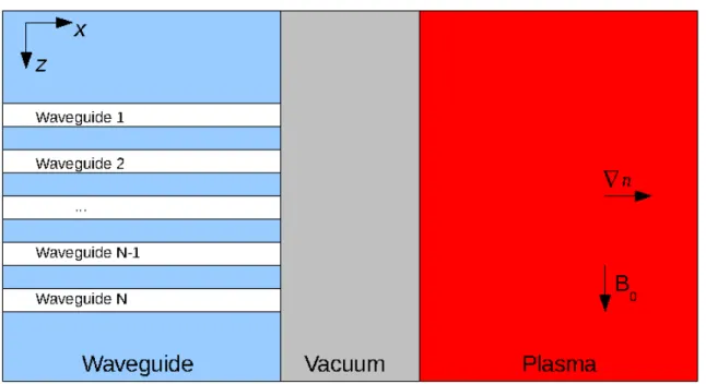
3-1 Slab geometry for the coupling problem. . . 80

3-2 One-dimensional wave field solution at the plasma edge. . . 83

(13)

3-4 LH wave coupling as a function of edge density. . . 89

3-5 Directional couplers in LH launcher. . . 91

3-6 Waveform for low power coupling experiments. . . 92

3-7 Non-perturbing L-mode coupling results . . . 93

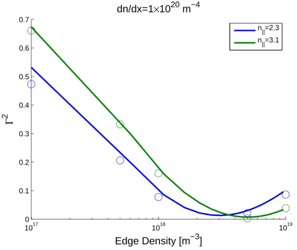
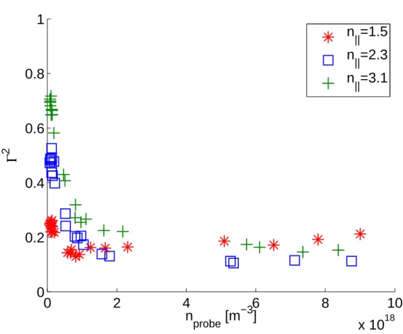
3-8 Reflection coefficient vs. probe density with variable gradient model. 95 3-9 Reflection coefficient vs. probe density with vacuum gap model. . . . 97

3-10 Reflection coefficient vs. probe density with density scale length model. 98 3-11 Two possible edge density profiles which agree with the LH Langmuir probe measurement. . . 100

3-12 Edge density change during long pulse, high power operation. . . 101

3-13 Coupling measurements at high power. . . 102

3-14 LH wave coupling in the presence of ICRF in L-mode. . . 104

3-15 Magnetic field line map of ICRF and LH antennas. . . 105

3-16 LH coupling during H-mode. . . 107

3-17 LH coupling during ohmic H-mode. . . 108

3-18 LH wave coupling for H- and L-mode discharges with ICRF. . . 109

3-19 Location of gas puffing capillaries as seen from inside the tokamak. . 110

3-20 Image of LH launcher with gas puffing on and off. . . 111

3-21 LH probe density vs line averaged density during gas puffing. . . 112

4-1 Visible plasma emission during high power LH. . . 117

4-2 Comparison of visible plasma emission during high power LH. . . 118

4-3 Time history of visible emission on the LH launcher. . . 119

4-4 Changes in brightness and density during high power LH operation. . 122

4-5 Melting of D row waveguide septa. . . 125

4-6 Solution of 1D heat equation. . . 128

4-7 Shape mismatch between plasma and LH launcher. . . 130

4-8 Formation of leading edges on the LH launcher septa. . . 131

(14)

4-10 Spectrum of launched n|| including high harmonics. . . 137

4-11 Injection from LH launcher caused by D-port ICRF antenna. . . 139

5-1 Accessibility in high density L-mode. . . 143

5-2 Hard X-ray emission versus line averaged density, linear scale. . . 144

5-3 Hard X-ray emission versus line averaged density, semi-log scale. . . . 145

5-4 Hard X-ray emission versus line averaged density, normalized to net LH power. . . 146

5-5 Hard X-ray emission versus line averaged density, no normalization. . 147

5-6 Fast electron bremsstrahlung emission as a function of n||crit− n||launch. 149 5-7 Fast electron bremsstrahlung as a function of ω/ωLH. . . 151

5-8 Frequency spectrum showing weak Parametric Decay Instability. . . . 152

5-9 PDI Level as a function of density and ω/ωLH. . . 153

5-10 Pump wave width as a function of line averaged density. . . 154

5-11 Magnetic field line map of A-port Scanning Probe and LH antenna. . 156

5-12 LHRF wave fields in SOL. . . 157

5-13 LHRF wave fields in SOL as a function of line averaged electron density.158 5-14 I − V characteristic for Langmuir probes. . . 160

5-15 Divertor Langmuir probe geometry. . . 161

5-16 Location of divertor Langmuir probes. . . 162

5-17 Waveform of SOL currents observed during LHCD experiments in LSN. 163 5-18 Waveform of SOL currents observed during LHCD experiments at high density in USN. . . 164

5-19 SOL current direction in USN and LSN. . . 165

5-20 SOL current density versus line averaged density. . . 166

5-21 Ratio of Ignd to Isat on divertor probes in LSN. . . 168

5-22 Simulated and measured HXR emission as a function of density. . . . 172

5-23 GENRAY simulation showing rays trapped near the edge. . . 173

(15)

5-25 Accessibility limited ray in a slab geometry. . . 175 5-26 Simulated HXR Emission with Limited Radial Reflections . . . 177 5-27 Mid-plane density profile with SOL model. . . 179 5-28 GENRAY simulation of ray trajectories in the SOL at high density. . 180 5-29 GENRAY simulation of ray trajectories in the SOL at high density. . 181 5-30 Comparison of simulated X-Ray emission with and without SOL model

in GENRAY. . . 182 5-31 Comparison of simulated X-Ray emission with 2-D SOL model in

GEN-RAY. . . 183 5-32 Ray trajectories including a 2-D SOL model and reflections from the

vacuum vessel. . . 184 5-33 Radial profile of density fluctutations. . . 187 5-34 Simulated X-Ray emission with scattering from density fluctuations

with no SOL. . . 188 5-35 Sensitivity of simulated X-Ray emission with respect to density

fluc-tuation amplitude. . . 189 5-36 Sensitivity of simulated X-Ray emission with respect to Nφ of density

fluctuations. . . 190 5-37 Imaginary component of k⊥ due to electron-ion collisions at 4.0 T. . . 192

5-38 Simulated X-Ray emission including collisional damping in the SOL. . 193 5-39 Hyperbolic tangent density profile. . . 196 5-40 1-D full wave simulation showing penetration of waves through a tanh

density pedestal, n|| = 1.55. . . 197

5-41 1-D full wave simulation showing penetration of waves through a tanh density pedestal, n|| = 2.33. . . 198

(16)

5-45 Transmission through pedestal as a function of density and density gradient. . . 204 5-46 Changes in H-mode profiles with the application of LHCD. . . 206 5-47 Changes in H-mode pedestal parameters with the application of LHCD. 207 5-48 Low density H-mode with LH induced pedestal modification. . . 208 5-49 HXR emission as a function of line averaged density during H-mode. . 210 5-50 HXR emission minus background as a function of line averaged density

during H-mode. . . 211 5-51 Ray trajectories in a low density H-mode with no SOL model. . . 212 5-52 Ray trajectories in a low density H-mode with SOL model. . . 213 5-53 Comparison of experimental and simulated HXR emission with no SOL

model during H-mode. . . 214 5-54 Comparison of experimental and simulated HXR emission with 2-D

SOL model during H-mode. . . 215

A-1 Histogram of phase difference between calibrations. . . 231 A-2 Change in n||spectrum due to error in waveguide phasing and amplitude.232

(17)

(18)

List of Tables

1.1 World energy reserves and time remaining based on current rate of consumption. . . 20

2.1 Alcator C-Mod Device Parameters . . . 59 2.2 Waveguide Properties. . . 63 2.3 Comparison of C-Mod LHCD System with Other Recent and Current

Experiments . . . 76

3.1 GRILL Code Namelist Variables . . . 88

4.1 Changes in Dα brightness and electron density on the LH launcher at

high power. . . 121

A.1 Thru-phase launcher calibration performed on 07/02/2008. . . 229 A.2 Difference in thru-phase calibration from 10/26/2007 to 07/02/2008. . 230

(19)

(20)

Chapter 1 Introduction

For much of human history, energy needs have been met in a largely sustainable manner with locally available resources. Heating, cooking, and lighting were pro-vided largely by burning biomass, while transportation needs were met by beasts of burden or wind power. Still, examples exist of resource exhaustion and subsequent societal collapse, such as the Rapanui of Easter Island and the Norse settlements on Greenland. With the start of the Industrial Revolution, however, demand for energy to run new machinery rose dramatically. The energy needs of industrialized regions quickly outpaced the rate at which traditional renewable fuels could be replenished, at which point coal and oil were extracted from the earth in ever increasing quantities. Two centuries after the start of the Industrial Revolution, the world’s appetite for fossil fuels continues to surge. Estimates for the remaining reserves of oil, natural gas, and coal range from 20-200 years at current rates of consumption (see Table 1.1). In addition to the imminent exhaustion of fossil fuels, the mass release of carbon diox-ide and other greenhouse gases into the atmosphere is pushing the earth towards a tipping point beyond which global climate change will be inevitable. As a result of these trends, there has been great interest in using non-fossil fuels for the generation of electricity as it can be easily transported over long distances converted into other forms of useful energy such as heat, light, and mechanical movement.

(21)

Table 1.1: World energy reserves [1]. Time remaining is the number of years until the resource is exhausted assuming assuming a usage rate of 500 Quads/y (the estimated 2010 world energy use rate [2]). The time remaining is extended if a combination of multiple fuel sources is utilized.

Resource Reserves [Quads] Time remaining [y]

Coal 105 ₂₀₀ Oil 104 ₂₀ Natural Gas 104 ₂₀ Fission (U235₎ ₁₀4 ₂₀ Fission (U238_-Th232_{) 10}7 _{2 × 10}4 Fusion (D-T) 107 _{2 × 10}4 Fusion (D-D) 1012 _{2 × 10}9

1.1 Fusion Basics

Many “renewable” sources of energy have found proponents in recent years as the end of fossil fuel reserves looms on the horizon. Wind and solar power are intermit-tent resources that cannot provide the consisintermit-tent base load generation necessary to maintain a reliable electric grid. Consequently, intermittent resources cannot exceed approximately 20% of the installed generating capacity without destabilizing the elec-tric grid. Hydroelecelec-tric dams can provide steady state elecelec-tric production with no emissions, however most major rivers in the industrialized world have already been fully tapped for hydroelectric projects. Although hydroelectric electricity production is renewable and does not release any pollutants, it has a substantial negative impact on the river ecosystem by disrupting the natural flow of sediment and interfering with the migration of anadromous fish.

Although not strictly speaking a “renewable” resource, nuclear energy can fill the gap left when fossil fuel sources run out without contributing to climate change. The source of nuclear energy is the strong force inside the nucleus, which is 102 _{times more}

powerful than the electromagnetic forces which form chemical bonds, and 1038 _times

(22)

0 10 20 30 40 50 60 70 80 90 100 −4 −2 0 2 4 6 8 10x 10 6

Atomic Number

Binding Energy per Nucleon [eV]

Fusion

Fission

Figure 1-1: Nuclear binding energy per nucleon as a function of atomic number peaks for Fe. The most abundant isotope for each element is plotted [3].

force binds the protons and neutrons in the nucleus together, and is strongest for Fe56_{. Heavier and lighter elements are less tightly bound, and consequently energy}

is released when lighter elements combine together (fusion) or heavier elements split apart (fission). Figure 1-1 shows the binding energy per nucleon as a function of atomic number. Fusion is achieved by moving up from the left side of the peak, while fission is achieved by moving up from the right side of the peak.

Nuclear fission, which has for decades been a workhorse of electric utilities, is attractive as a near-term source of energy. Uranium fuel is for the time being still plentiful, and many of the difficult engineering challenges in designing a safe, reliable fission power plant have been solved. Both fission and fusion reactors can in principle provide a steady base load which is not dependent on the weather unlike solar and wind power.

(23)

radioactive with long half-lives, and a suitable long-term storage facility for this waste has not been selected in the United States at this time. In addition, public concern regarding the safety of fission power plants has been a major obstacle to the construc-tion of new facilities, and the proliferaconstruc-tion of weapons-grade fissile materials limits the attractiveness of fission power production in less stable regions of the world. As com-pared to fission, nuclear fusion is very attractive as a long-term energy solution. The byproducts of a fusion reaction have short half lives, mostly on the order of minutes to months, as compared to thousands or millions of years for fission byproducts.

The fuel considered for most fusion reactor studies is comprised of deuterium and tritium. Deuterium is a naturally occurring isotope with a relative abundance of 0.015% of hydrogen on earth. Even though deuterium accounts for a very small fraction of the hydrogen supply, the vast oceans contain enough deuterium to power the world for approximately 1012 _{years. Tritium is not a naturally occurring isotope,}

however it can be “bred” by bombarding lithium with neutrons to produce helium and tritium.

1.2 Fusion Reactions and Ignition

The positive slope of the curve in Figure 1-1 between H and Fe suggests that several fusion reactions of light elements are possible, however the greatest change in binding energy, and therefore energy release, occurs for the fusing of hydrogen isotopes on the far left end of the curve. Among these are the D-D reaction and the D-T reaction. Other more exotic fusion reactions, such as D-3_{He and H-}11_{B, exist although the rarity}

of fuel for these reactions makes them less interesting than the hydrogenic reactions. The power released in a fusing plasma is

Pf us = nanbhσviQf us (1.1)

(24)

fusing species (for like particle reactions, nanb = n2_{/2), σ is the cross section of the}

reaction, v is the relative velocity of the two particles, and Qf usis the energy released

per fusion reaction. Here, h. . .i represents an average over a Maxwellian distribution function at a temperature T .

To achieve a self-sustaining chain reaction (a “burning plasma”), it is necessary that the fusion power released to the plasma from the fusion reaction exceed the power lost from the plasma through radiation and conduction. The conditions necessary for thermonuclear fusion were first addressed by Lawson in an initially classified report [4] and later in a published journal [5]. Assuming a D-T fusion reaction, this results in the inequality

Pf us− Ploss≥ 0 nDnThσviQα− W/τE ≥ 0

(1.2)

where Qα = 3.5 MeV is the energy of the helium nucleus coming from the D-T fusion

reaction. Here we have taken that the energy loss rate from the plasma is equal to the thermal energy stored in the plasma, W , divided by the energy confinement time,

τE of the plasma. For a thermal plasma

W = 3nkT (1.3)

which leads to the “Lawson Criterion” [3]

neτE ≥

12kT

Qαhσvi (1.4)

where we have assumed nD = nT = ne/2. The right hand side of Equation 1.4 has a

minimum at 25 keV of approximately 1.5 × 1020 _m−3_{s. The top panel of Figure 1-2}

shows hσvi as a function of temperature for the D-D, D-T, and D-3_{He reactions. The}

bottom panel shows the minimum value of nτ necessary for ignition as a function of temperature for the D-T reaction. This simple analysis does not include the power

(25)

radiated by the plasma through bremsstrahlung which sets a minimum temperature of ∼ 4.4 keV for ignition.

There are two primary approaches used to simultaneously achieve the n, τ and

T required for ignition. The first approach, inertial confinement, uses a shock-wave

to compress a small volume of plasma to extremely high densities and temperatures. This results in a miniature explosion as the plasma burns. Inertial confinement does not lend itself readily to large scale electricity production since it is by its nature a pulsed power source.

As suggested by its name, magnetic confinement fusion uses magnetic fields to confine the fusing plasma. To first order, the Lorentz force on a charged particle moving perpendicular to a magnetic field causes that the particle to gyrate around the field rather than transit across the field. If the magnetic field forms a closed path without intersecting any physical objects, a magnetic surface is created in which the plasma can be confined.

1.3 Tokamaks

To date, the highest performance magnetic confinement concept is the tokamak. The tokamak uses a combination of toroidal, poloidal, and vertical magnetic fields to confine the plasma inside a toroidal vacuum vessel. The toroidal and vertical fields are imposed by external electromagnets, while the poloidal field is generated by a current flowing toroidally through the plasma itself. In the absence of any of these three key magnetic fields, instability will quickly thrust the plasma into the vacuum vessel wall, thereby quenching the plasma and possibly damaging the tokamak.

The combination of a toroidal and poloidal magnetic fields result in a total mag-netic field such that any given line of magmag-netic field will wrap in a helical manner around the torus, and will eventually map out a surface known as a flux surface. If the flux surface intersects a solid structure such as the vacuum vessel, it is called an

(26)

100 101 102 103 10−35 10−30 10−25 10−20

T [keV]

<

σ

v> [m

3

s]

_D−T D−D D−3He 100 101 102 103 1020 1021 1022 1023 1024

T [keV]

n

τ

[m

−3

s]

Figure 1-2: Fusion cross sections hσvi as a function of temperature for the D, D-T, and D-3_{He reactions [6]. (top) Minimum value of nτ necessary for ignition as a}

function of temperature for the D-T reaction. The effect of bremsstrahlung emission is ignored in this calculation. (bottom)

(27)

open flux surface, while flux surfaces not contacting a solid structure are closed flux surfaces. The boundary between these two regions is known as the separatrix or last closed flux surface (LCFS). The region of open flux surfaces is commonly referred to as the scrape-off-layer (SOL).

1.4 Current Drive and Steady State Operation

For reliable electricity generation, it is desirable to have a steady-state reactor which can fulfill the base load generation requirements, however the conventional tokamak is an inherently pulsed device. A toroidal current is required to maintain plasma stability, and this toroidal current is typically provided through mutual induction with an electromagnet as the primary coil and the plasma itself as the secondary coil of the transformer. By using the integral form of Faraday’s Law, the voltage induced around a closed toroidal contour in the plasma is

Vloop= I C ~ E · d~l = −∂ ∂t Z Z S ~ B · d ~A = −∂ψ ∂t (1.5)

To create a steady state toroidal current in the plasma through inductive current drive

Vloop must be held constant, however it is not possible to maintain a constant ∂ψ/∂t

indefinitely. For a solenoidal electromagnet, ψ ∝ IOH where IOH is the current flowing

through the transformer magnet and ψ is the magnetic flux through the coils of the magnet. It would therefore require a power supply with no current limit, as well as a magnet which can withstand an infinite current, to sustain a steady state tokamak plasma. In practice, the transformer is run in a “double swing” configuration where the starting current in the magnet is at the negative limit, and the current is then ramped through zero to the positive limit or vice-versa, but this can only increase the maximum pulse length by a factor of 2.

The limitations of a pulsed tokamak can be overcome by the addition of non-inductive current drive mechanisms. Current can be driven non-non-inductively through

(28)

the application of high power neutral beams and microwaves, and even by the plasma itself under the correct conditions.

1.4.1 Neutral Beam Current Drive

Neutral beams can be used as both a source of auxiliary heating and non-inductive current drive in a tokamak. A charged particle beam cannot be used for current drive since the gyromotion of the charged particle will prevent penetration across the magnetic field into the core plasma. Although the physics of beam current drive are relatively simple and robust, the biggest detriment of neutral beams are the size, cost, and complexity of the beams. High energy, high current neutral beams require large structures to accelerate an ionized beam followed by a neutralization process. This neutralization process is not highly efficient and many of the high energy ions are not converted into high energy neutrals.

1.4.2 Microwave Current Drive

Non-inductive current drive can also be achieved with high power microwaves under certain conditions [7]. Electron Cyclotron Current Drive (ECCD) relies on preferen-tially heating electrons moving in one toroidal direction to create an asymmetry in the resistivity of the plasma.

Lower Hybrid Current Drive (LHCD) utilizes a more direct current drive mecha-nism. Lower Hybrid (LH) waves are launched in one toroidal direction and directly deposit the wave momentum and energy on electrons traveling roughly in phase with the waves. These electrons, which move at relativistic velocities and are relatively col-lisionless, can drive a significant current even if they are few in number. The current drive mechanism for LH waves will be discussed in detail later in this chapter.

As compared to ECCD, LHCD has a much higher current drive efficiency as measured in driven current per unit power. This makes LHCD a very desirable means for driving current, however LHCD is not without its drawbacks. Unresolved physics

(29)

and engineering issues such as poor edge coupling during ion cyclotron resonance heating (ICRH), loss of current drive efficiency at high density, and survivability of the LHCD antenna still exist. An analysis of these issues comprises the bulk of this thesis.

1.4.3 Bootstrap Current

The “bootstrap current” is a self driven plasma current which requires no external input under the appropriate conditions. The reader may consult a review by Peeters [8] for a complete treatment of the physical process leading to the bootstrap current as only a simple description will be included here. The bootstrap current arises due to the effects of trapped electrons in the presence of pressure gradients in the plasma. As the trapped electrons traverse toroidally, they follow banana-shaped orbits as viewed in the poloidal plane. The electrons travel one direction toroidally on the inside of the banana, and the opposite direction on the outside of the banana. If a density gradient exists in the plasma, there will be a difference in the number of trapped electrons traveling one direction toroidally versus the other at a given point in space, which will generate a net current. By a similar argument, a temperature gradient in the plasma will generate electrons moving faster in one toroidal direction as compared to the opposite, thereby generating a net current. The direction of the current created by these trapped electrons is fortuitously in the same direction as the main plasma current.

Although the bootstrap current is not directly driven by external means, as is the case with NBCD, ECCD, and LHCD, it must be noted that generating the steep pressure gradients necessary to sustain the bootstrap current generally requires the application of external heating, and in practice it is impossible to create a plasma with 100% bootstrap current. Most proposed non-inductive tokamaks rely on bootstrap current for at most 70% of the total current with RF or neutral beams supplying the balance.

(30)

1.5 LH Background Physics

The propagation of electomagnetic waves in a plasma can be studied by first consid-ering Maxwell’s Equations

∇ × ~E = −∂ ~B ∂t (1.6a) ∇ × ~B = µ0J +~ 1 c2 ∂ ~E ∂t (1.6b)

as well as Ohm’s Law

~

J = σ · ~E (1.7)

where σ is the anisotropic conductivity of the plasma. Equations 1.6a, 1.6b, and 1.7 can be combined to form

∇ × ∇ × ~E = −1 c2 ∂2_E~ ∂t2 − ∂ ∂t(µ0σ · ~E) (1.8)

Assuming variations of the wave field of the form ei(~k·~x−ωt)_{, we can Fourier analyze}

this equation, taking ∇ = i~k and ∂

∂t = −iω. The equation can thus be simplified to ~k × ~k × ~E + iωµ0σ · ~E + ω2 c2E = 0~ (1.9) Substituting ~n = c~k ω

into Equation 1.9 results in

~n × ~n × ~E + ² · ~E = 0 (1.10)

where

² ≡ I +ic2µ0

(31)

which then simplifies to

(~n~n − n2_{I) · ~}_{E + ² · ~}_{E = 0} _(1.12)

By taking ~n = n⊥x + nˆ ||z, Equation 1.10 can be written in matrix form asˆ

     ²⊥− n2_|| −i²× n⊥n|| i²× ²⊥− n2 ||− n2⊥ 0 n||n⊥ 0 ²||− n2⊥     · ~E = 0 (1.13)

where ²⊥, ²×, and ²|| are the elements of ²

² =      ²⊥ −i²× 0 i²× ²⊥ 0 0 0 ²||      (1.14)

At this point, it is convenient to derive the elements of the conductivity tensor,

σ. We begin with momentum conservation for a charged particle in the presence of a

magnetic field

q( ~E + ~v × ~B) = m∂~v

∂t (1.15)

where q is the (signed) charge of the particle, m, is the mass of the particle, ~v is the velocity of the particle, and ~E and ~B are the electric and magnetic fields. Here we

will assume ~E = ~E1, ~B = ~B0 + ~B1, and ~v = ~v1 where the subscript zero indicates

background quantities and the subscript one indicates perturbed quantities. The zeroth order components of the velocity and the electric field are taken to be zero. Again, we can replace ∂

∂t with −iω, which leads to

q( ~E1+ ~v1× ~B0) = −iωm~v1 (1.16)

if we only retain first order quantities. It should be noted that this equation is valid for both ions and electrons. Each must be solved for independently and their

(32)

contributions added together. We assume ~B0 = B0z without any loss of generality.ˆ

Solving for the components of ~v1 results in v1x = iq mω(E1x+ v1yB0) v1y= iq mω(E1y− v1xB0) v1z = iq mωE1z (1.17)

Solving this system of equations results in

v1x= 1 1 − ω2 c/ω2 µ iq mωE1x− q2_B 0 m2_ω2E1y ¶ v1y = 1 1 − ω2 c/ω2 µ iq mωE1y+ q2_B 0 m2_ω2E1x ¶ v1z = iq mωE1z (1.18)

From Equation 1.18 we can form the matrix σ by using the relation that ~J =Pnq~v

σ =X q 2_n m      iω ω2_−ω2 c −ωc ω2_−ω2 c 0 ωc ω2_−ω2 c iω ω2_−ω2 c 0 0 0 i ω      (1.19)

where the sum is performed over the electrons and all ion species. We can now express the elements of Equation 1.11 as

² =      1 −P ωp2 ω2_−ω2 c − P iωcω2p ω(ω2_−ω2 c) 0 P _iω_c_ω2 p ω(ω2_−ω2 c) 1 − P _ω2 p ω2_−ω2 c 0 0 0 1 −Pω2p ω2      (1.20) where ωc= qB/m and ωp = p nq2_/m² 0.

(33)

matrix and set it equal to zero. The result is the wave dispersion relation, denoted as D(ω, ~k) = ¯ ¯ ¯ ¯ ¯ ¯ ¯ ¯ ¯ ²⊥− n2_|| −i²× n⊥n|| i²× ²⊥− n2||− n2⊥ 0 n||n⊥ 0 ²||− n2⊥ ¯ ¯ ¯ ¯ ¯ ¯ ¯ ¯ ¯ = 0 (1.21)

If we take n|| as a fixed value set at the edge by the antenna structure, we can solve

Equation 1.21 for n⊥. This leads to a fourth order bi-quadratic equation for n⊥

0 = C4n4⊥+ C2n2⊥+ C0 (1.22)

where

C4 = ²⊥ (1.23a)

C2 = (n2||− ²⊥)(²||+ ²⊥) + ²2× (1.23b) C0 = ²||((n2||− ²⊥)2− ²2×) (1.23c)

Equation 1.22 can be solved for n2

⊥ using the quadratic equation

n2 ⊥ = −C2± p C2 2 − 4C4C0 2C4 (1.24)

The first (+) root of Equation 1.24 is known as the slow wave, while the second (-) root is the fast wave. These names come from the perpendicular phase velocities of the two waves, vph⊥ = ω/k⊥= c/n⊥, which is larger for the fast wave and smaller for

the slow wave.

1.5.1 Accessibility

Equation 1.24 shows that distinct slow and fast wave modes can propagate for a single value of n|| provided that the discriminant is locally greater than zero. When the two

(34)

Figure 1-3 shows the two roots of the cold plasma dispersion relation for typical C-Mod parameters. The n|| = 1.55 case exhibits a violation of the accessibility criterion

when the local electron density reaches 5 × 1019 _m−3 _{with a local magnetic field of}

5.0 T. At this density, the discriminant approaches zero and the fast and slow wave branches of the dispersion relation coalesce. In this case, a slow wave launched from a lower density region near the edge of the plasma will reflect back as a fast wave, and vice versa. The point at which the discriminant goes to zero is known as the mode conversion layer. Higher values of n|| are accessible to higher densities for a given

value of magnetic field. Since the slow wave is the desirable branch for current drive (the reason for which will be discussed in Section 1.5.4), it is necessary to prevent the launched waves from reaching any point in the plasma where the accessibility criterion is violated.

The inequality

C₂2− 4C4C0 > 0 (1.25)

can be simplified for LH waves with some ordering of the terms in C4, C2, and C0.

First, we consider how the launched LH wave frequency, ω, compares to the cyclotron and plasma frequencies for electrons and ions in a tokamak. For ions, ω À ωci and ω > ωpi, while for electrons ω ¿ ωce and ω < ωpe. This allows us to approximate

the elements of ² as ²⊥ ≈ 1 − ωpi2/ω2 + ω2pe/ωce2 , ²× ≈ ω2pe/ωωce, and ²|| ≈ −ω2pe/ω2,

which leads to an ordering ²⊥ ∼ 1, ²× > 1, and |²||| À 1. We can therefore simplify

Equation 1.23 as

C4 = ²⊥ (1.26a)

C2 = (n2||− ²⊥)(²||) + ²2× (1.26b) C0 = −²||²2× (1.26c)

Plugging these values into Equation 1.25 results in ¡

(n2_||− ²⊥)²||+ ²2×

¢₂

(35)

0 0.5 1 1.5 2 2.5 x 1020 −1000 −500 0 500 1000 1500 2000 2500 3000 3500 4000

Fast and slow wave dispersion relation, B=5T, f=4.6GHz

Local n

e

n

⊥ 2 n ||=1.55 n ||=2.33 n ||=3.1 Slow Wave Fast Wave

Figure 1-3: LH dispersion relation for B = 5.0 T, f = 4.6 GHz. Solid lines represent the real part of n2

(36)

Solving this equation for n2

|| and factoring yields

n2_|| > Ã √ ²⊥+ s −² 2 × ²|| !2 (1.28)

Finally, substituting the simplified elements of ² gives the accessibility criterion as

|n||| > s 1 −ω 2 pi ω2 + ω2 pe ω2 ce + ωpe |ωce| (1.29)

The condition for the accessibility of LH waves was first correctly identified by Golant [9]. Troyon and Perkins [10] derived the approximate accessibility criterion of Equa-tion 1.29. The accessibility profile along the midplane of a hypothetical C-Mod plasma with a parabolic density profile is shown in Figure 1-4.

1.5.2 Wave Launching

Lower Hybrid waves in the low GHz frequency range are often launched from phased arrays of waveguides operating in the fundamental TE10 mode. The waveguides are

oriented such that the wave electric field in the waveguide is nearly parallel to the background magnetic field in the plasma. For the TE10 mode, the wave electric field

is directed across the narrow dimension of the waveguide. This orientation of the electric field assures that the slow wave branch of the dispersion relation, for which the wave electric field is also parallel to the background magnetic field, is excited. Multiple waveguides are located in a row with adjacent waveguides separated by a thin septum. The interference of waves launched from each of the waveguides results in an electric field pattern with a characteristic spectrum in k||. The k|| spectrum can

be determined by performing a Fourier transform in real space along the direction of the magnetic field

Ez(kz) = F(Ez(z)) ≡

Z _∞

−∞

e−ikzz_E

(37)

0.650 0.7 0.75 0.8 0.85 0.9 1 2 3 4 5 6

R [m]

n ||crit n e [10 20_m−3_] B [T]

Figure 1-4: Critical n|| for LH wave accessibility on the mid-plane of a tokamak as a

function of major radius for a parabolic density profile. The magnetic axis is at 0.67 m and the plasma edge is at 0.9 m.

(38)

where the magnetic field is in the ˆz direction and f (z) is the complex electric field at

the waveguide mouth. Taking n||≡ ckz/ω, the Fourier spectrum is

F (n||) = Z _∞

−∞

e−in||ω_cz_{f (z)dz} _(1.31)

The electric field at the waveguide mouth can be expressed as a sum of rectangle functions. The rectangle function is a single square pulse of width 1 centered about the origin

rect(x) = u(x + 1/2) − u(x − 1/2) (1.32)

where u(x) is the Heaviside function. The electric field is thus

Ez(z) =

N −1_X

j=0

Ejrect([z − (j(w + δ) + w/2)]/w)e−iφj (1.33)

where Ej is the magnitude of the electric field, w is the waveguide width, δ is the

septum width, and φj is the phase of the electric field. The subscript j refers to

the value of the quantity for the jth _{waveguide. The top panel of Figure 1-5 shows}

the magnitude and phase of the electric field for a 10 waveguide array with a phase difference between adjacent waveguides of π/2.

The Fourier transform for a single rectangular pulse of width w centered at z = 0 is given by the sinc function

F(rect(z/w)) = sin(kw/2)√

2πk/2 (1.34)

Making use of the property of Fourier transforms that

(39)

the Fourier transform of Equation 1.33 is Ez(n||) = N −1 X j=0 Ej sin(n_√ ||wω_2c) 2πn||_2cω e−i(β+φj) _(1.36) where β = n|| ω c(j(w + δ) + w/2) (1.37)

The power spectrum as a function of n|| is proportional to EzEz∗. This gives

P (n||) ∝ sin2_(n ||wω_2c) n2 || N −1_X j=0 Eje−i(β+φj) N −1 X j=0 Ejei(β+φj) (1.38)

If the value of Ej is the same for each waveguide, then this term can be moved outside

the sum. If we take φj = j∆φ, where ∆φ is the phase difference between adjacent

waveguides in radians, and neglect the w/2 term in β (which comes only from an initial shift of position in real space and does not effect the power spectrum), we can rewrite the sum

N −1_X j=0 e−i(β+φj)₌ N −1_X j=0 e−i(n||ωc(w+δ)+∆φ)j = N −1_X j=0 e−iαj (1.39)

Making use of the identity

N X j=1 xj = x1 − x N 1 − x (1.40)

the sum can be eliminated. This results in a power spectrum

P (n||) = P0 sin2_(n ||wω_2c) n2 || sin2_(Nα/2) sin2_(α/2) (1.41) where α = ³ ∆φ + n|| ω c(w + δ) ´ (1.42)

(40)

−0.02−2 0 0.02 0.04 0.06 0.08 0.1 0 2 4

z [m]

|E z| [a.u.] arg(E z) [rad] −100 −8 −6 −4 −2 0 2 4 6 8 10 0.2 0.4 0.6 0.8 1

n

||

P(n

||

) [a.u.]

Figure 1-5: Amplitude and phase of electric field for the forward wave in an LH launcher with 10 waveguides. Waveguide width is 0.0055 m and septum width is 0.0015 m. The phase difference between adjacent waveguides is π/2. (top) Fourier transform of the top panel showing the n|| spectrum. (bottom)

shown in the bottom panel of Figure 1-5. A convenient formula for the peak of the

n|| spectrum is

n|| =

c∆φ

2πf (w + δ) (1.43)

By adjusting the phase difference between adjacent waveguides, the peak of the spec-trum can be tuned to a desired value. It should be noted that this treatment is valid only for the ideal case where there is no variation in amplitude nor errors in phas-ing among the waveguides. Slight differences in the low amplitude sidebands of the spectrum can result from these imperfections.

(41)

1.5.3 Wave Damping

The cold plasma treatment of Lower Hybrid waves treats propagation without in-troducing any losses. However, a hot plasma treatment of the plasma including the effects of finite electron temperature results in both propagation and damping of the waves. This hot plasma description includes the effects of wave-particle resonances, which lead to imaginary components of the dispersion relation and therefore wave damping. For the purposes of current drive with LH waves, Landau damping is the dominant absorption mechanism. Landau damping is a collisionless damping process by which charged particles and waves traveling with nearly the same phase velocity parallel to the magnetic field exchange energy and momentum. In principle, Landau damping is possible for both electrons and ions, however the ion absorption rate is typically negligible due to their lower thermal velocity.

To derive the hot plasma dispersion relation, we follow a similar procedure as for the cold plasma case, however we take the current to be the moment of the distribution function

~ J = n0

Z Z Z

(qe~vfi(~v) + qe~vfe~v) d3~v (1.44)

where fi(~v) and fe(~v) are the normalized distribution functions for ions and electrons,

and qm is the charge of species m. We now will examine how these distribution

func-tions are perturbed by the waves, beginning with a Maxwellian distribution function

f0 = 1 (2π)3/2_v3 t e− v2_⊥+v_||2 2v2_t _(1.45) where vt = p

T /m is the thermal velocity. This distribution function is valid for both

electrons and ions. We then consider a linearized Vlasov equation

∂ ∂tf1+ ~v · ∇f1+ q m~v × ~B0· ∇vf1 = q m ³ E1+ ~v × ~B1 ´ · ∇vf0 (1.46)

(42)

components. Again, this is valid for both ions and electrons. This equation can be solved by integrating particle orbits along ~B0. The result is used in the derivation

of the dispersion relation, which separates into real and imaginary parts D(ω, ~k) =

Dr(ω, ~k) + iDi(ω, ~k) [11]. The real part of D is identical to the cold plasma dispersion

relation except for the addition of a n6

⊥ term. The imaginary part of D contains two

terms, the first of which is due to electrons and the second of which is due to ions

Di = 2√π µ ω2 pe ω2 n 2 ⊥n2||x3ee−x 2 e + ω 2 pi ω2n 4 ⊥x3ie−x 2 i ¶ (1.47) where xe = ω/( √ 2k||vte) and xi = ω/( √

2k||vti). It is this imaginary part of D which

gives rise to the damping of the LH waves. It can be seen that, except for very slow waves or very hot ions, xi ¿ 1 and therefore the ions will not contribute substantially

to the damping process. To solve for the imaginary part of k⊥, we make a Taylor

expansion of D around k⊥r

D(ω, ~k) = D(ω, k⊥r) + (k⊥− k⊥r) ∂D ∂k⊥r

+ . . . = 0 (1.48)

Since both k⊥ and D are both complex quantities, we can rewrite this expansion as

Dr+ iDi+ ik⊥i ∂Dr ∂k⊥r − k⊥i ∂Di ∂k⊥r + . . . = 0 (1.49)

The real and imaginary parts of this equation can be set to zero and be solved for k⊥r

and k⊥i. The fourth term in Equation 1.49 is second order and is therefore negligible.

Assuming we have a normal mode of the system Dr(k⊥r, ω) = 0, the expression for k⊥i is

k⊥i = − Di ∂Dr/∂k⊥r

(1.50)

(43)

making use of ²⊥ ∼ 1 and ²|| ∼ −ωpe2 /ω2 results in k⊥i = √ πωpe c n||x 3 ee−x 2 e (1.51)

The maximum of k⊥i, and thus the strongest damping, is located at xe = 3 √

2, or approximately ω/k|| = vte. For an electric field which varies as E0exp(i~k · ~x), the

power carried by the wave will decay exponentially as exp(−2k⊥ix), we can set the

condition for strong absorption in a tokamak, k⊥ia > 1, where a is the minor radius

of the plasma. Figure 1-6 shows the imaginary part of k−1_⊥ due to Landau damping as a function of n|| and Te. A value for k⊥i of 10−2 m corresponds to 86% of the

wave power absorbed in 1 cm of propagation perpendicular to the magnetic field, which would be strong single-pass absorption for C-Mod where a ∼ 20 cm. For a temperature of 2 keV, this requires n|| ≥ 4. This condition can also be expressed as

a general rule of thumb that the temperature in keV must be greater than 30/n2

|| for

strong single pass damping.

1.5.4 Current Drive Efficiency

The total current driven in the plasma is the first moment of the distribution functions for ions and electrons, however we will neglect the contribution from ions. Ions have a much lower velocity as compared to electrons which makes their contribution small. We then have

J|| = q

Z _∞

−∞

v||f||(v||)dv|| (1.52)

where J||is the current density parallel to the magnetic field, and f||(v||) is the electron

distribution as a function of v||. For a distribution function symmetric about v|| =

0, there is obviously no net current. We have already indicated in the preceding section that the distribution function is modified in the region near ω/k|| ∼ v||, which

leads to an asymmetric distribution function with a net J|| if the waves are launched

(44)

2 2.5 3 3.5 4 4.5 5 5.5 10−3 10−2 10−1 100

n

||

ℑ

k

⊥ −1

[m]

1 keV 2 keV 3 keV 4 keV

Figure 1-6: Landau damping e-folding length for LH waves as a function of Te and n||. A value for k⊥i of 1 × 10−2 m corresponds to 86.4% of the wave power absorbed

(45)

As discussed in Section 1.4.2, LHCD is highly very efficient as compared with other non-inductive current drive mechanisms. The following estimate of current drive efficiency is based on the argument of Fisch in Reviews of Modern Physics [7]. Current drive efficiency can be quantified as the ratio of the current driven to the power dissipated. This ratio can be expressed locally as J||/Pd. In a simple model,

the current driven by the lower hybrid waves is carried by a small population of electrons, δf , which is displaced in velocity space from v|| to v||+ δv||. Assuming that

the remainder of the distribution function is symmetric about v|| = 0, the net driven

parallel current is

J|| = qδv||δf (1.53)

Moving these electrons in velocity space requires an amount of energy, δE, equal to

δE = meδf 2 (v||+ δv||) 2₋meδf 2 v 2 ||≈ meδf v||δv|| (1.54)

for δv|| ¿ v||. These fast electrons have a finite lifespan prior to slowing down due

to collisions with the background plasma. The power necessary to sustain a steady state population of fast electrons can be estimated as the energy input per electron multiplied by the collision frequency of the electrons

Pd= ν(v)δE = meν(v)v||δf δv|| (1.55)

where ν(v) is the electron collision frequency and Pdis the local power deposition per

unit volume. We can now show that the efficiency is

J|| Pd =

q

mev||ν(v) (1.56)

This would suggest that more current can be driven with low v|| electrons, however we

have not considered the contribution of ν(v). Most of the electrons in the population

(46)

1.56 can be rewritten as J|| Pd ∝ v 2 || ne (1.57)

If these electrons are resonant with the parallel phase velocity of the lower hybrid wave, v|| = c/n||, we get a scaling that

J|| Pd

∝ 1 nen2_||

(1.58)

A more rigorous analysis of LHCD efficiency includes the effect of both direct momentum input and energy input [12]. The end result is

J|| Pd = 4 5 + Zef f ˆ s · ∇v(wu3) ˆ s · ∇vu2 (1.59)

where ˆs is the direction of velocity space displacement of the electrons, ∇v is the gradient in velocity space, w = v||/vte, and u = v/vte. The surprising consequence of

Equation 1.59 is that the current arising from energy input is three times the size of the term arising from momentum input.

Efficiency is typically compared between different tokamaks and current drive schemes using the figure of merit nIR/P T . Here, n is the line averaged density, I is the total plasma current, R is the major radius of the torus, and P is the net power used for current drive. This figure of merit comes from approximating that the driven current, and the power deposited, are distributed uniformly throughout an incremental area ∆A. This leads to

Ip = ∆AJ|| (1.60a)

and

P = ∆V Pd= 2πR∆APd (1.60b)

(47)

for J|| and Pd, we can show that J|| Pd

= 2πIR

P (1.61)

If we renormalize J|| and Pd to their thermal values

˜ J = J|| neevte (1.62a) ˜ Pd= Pd nemevte2ν0 (1.62b) we get ˜ J ˜ Pd = mevteν0 e J|| Pd (1.63) Using ν0 = ω4 peln Λ 2πnev3te (1.64)

and combining Equations 1.61 and 1.63 results in

η = nIR

P Te (1.65)

where η is the normalized current drive efficiency, frequently expressed in units of 1020_{A/(W m}2 _{keV). Values of η ∼ 0.1 are typical for LHCD on tokamaks.}

1.6 Ray Tracing, Full Wave, and Fokker-Planck

Simulation Codes

Self-consistent modeling of LH waves in a tokamak plasma is a difficult undertaking requiring the iterative use of two simulation codes. The first code determines the location of the waves in the plasma, either by ray tracing or through a full-wave approach. The wave code is used to evaluate the RF diffusion coefficient which is

(48)

then used in the Fokker-Planck solver to calculate the perturbed electron distribution function. Since the absorption of the waves, and consequently the wave electric field strength, is a function of the electron distribution, the perturbed distribution function is then passed back to the wave code, which recalculates the quasi-linear diffusion coefficient with the new distribution function. The process is repeated until the result converges.

Two methods are used to determine the propagation and damping of the waves in the plasma. The ray tracing approach makes use of WKB and geometrical optics approximations to represent waves as packets of photon energy traversing through the plasma. A series of “rays” are launched to approximate the wave-number spectrum produced by a three-dimensional antenna structure. These rays are independently followed through the plasma until they reach a damping threshold, at which point the ray is terminated. This approach is computationally simple but is fundamentally limited by the WKB approximation, which requires changes in wave characteristics to occur on scales long compared to the wavelength.

Another approach is to solve Maxwell’s Equations numerically. This correctly treats physical phenomena not addressed by ray tracing such as partial reflections, interference, and scattering, but at a substantial computational cost. To properly resolve the waves, the grid size and/or mode resolution used in the numerical method must be adequate to resolve the shortest wavelength in the system.

1.6.1 GENRAY

The GENRAY ray tracing package allows for the simulation of electromagnetic and electrostatic waves in a plasma medium through the use of the geometrical optics approximation [13]. The following outline of ray tracing derives from discussion in Landau and Lifshitz [14] and Weinberg [15].

First, we must introduce the concept of a “wave surface.” A wave surface is a two dimensional surface on which the amplitude and phase of a propagating

(49)

electromag-netic wave remain nearly constant over the distance of a wavelength. This allows for a plane wave approximation. On a wave surface, we can represent the electric and magnetic fields as follows

~ E = ~E0eiS(~x,t) (1.66a) ~ B = ~B0eiS(~x,t) (1.66b) where S(~x, t) (1.67)

is the eikonal, or phase, of the wave. On each wave surface, the normal vector to the surface represents the direction of propagation of the wave. A series of wave surface normals on successive wave surfaces forms a “ray” which defines the path of the wave.

For geometricical optics to be a valid approximation, the following relations must

be satisfied _¯ ¯ ¯ ¯λ_E_~1 0 ∂ ∂~xE~0 ¯ ¯ ¯ ¯ ¿ 1 (1.68a) and _¯ ¯ ¯ ¯λ_B_~1 0 ∂ ∂~xB~0 ¯ ¯ ¯ ¯ ¿ 1 (1.68b)

which are the requirements for a WKB approximation.

The eikonal S can be expanded in a Taylor Series as

S ' S0+ ~x ·∂S ∂~x + t

∂S

∂t + . . . (1.69)

Then by analogy with plane waves we can write

S = S0+ ~k · ~x − ωt (1.70)

where

~k = ∂S

(50)

ω = −∂S

∂t (1.71b)

Next consider an electromagnetic wave that satisfies the local dispersion relation

| ¯¯D| ≡ D0(~x, ~k, ω) = 0 (1.72)

We can construct ray paths ~x(τ ), ~k(τ ), ω(τ ), and t(τ ), where τ is a parameter rep-resenting the distance traveled along a ray path. These paths must satisfy the initial conditions ~x0 = ~x(τ0) ~k0 = ~k(τ0) ω0 = ω(τ0) t0 = t(τ0) ∇ × ~k(τ0) = 0 D0(~x0, ~k0, ω0, t0) = 0 (1.73)

Using the theory of characteristics it was shown by Weinberg [15] that the phase space solution of a wave that simultaneously satisfies Equation 1.73 is given by the ray equations d~x dτ = ∂D0 ∂~k (1.74a) dω dτ = ∂D0 ∂t (1.74b) d~k dτ = − ∂D0 ∂~x (1.74c) dt dτ = − ∂D0 ∂ω (1.74d)

If we take ∂D0/∂t = 0, we can use the chain rule to change from the step parameter τ to time t d dτ = d dt dt dτ = − ∂D0 ∂ω d dt (1.75)

(51)

This leads to d~x dt = − ∂D0 ∂~k ∂D0 ∂ω (1.76a) d~k dt = ∂D0 ∂~x ∂D0 ∂ω (1.76b)

GENRAY utilizes this framework to follow the ray trajectories for lower hybrid waves in an axisymmetric toroidal system. When calculated in the traditional manner, rays are launched from inside the edge of the plasma, and are allowed to propagate until they have damped beyond a user defined threshold. If the rays traverse to the edge of the plasma prior to fully damping, then they are reflected either off of a cutoff layer (if the density profile is such that a cutoff exists inside the plasma) or an artificial perfect conductor located at the plasma edge. The edge of the plasma is defined by the last closed flux surface from the EQDSK equilibrium file generated by EFIT.

GENRAY was recently modified to extend ray trajectories into the SOL, which was motivated in large part by the experimental observations detailed in Chapter 5. This new version of GENRAY allows the rays to propagate outside the separatrix provided that the local plasma density exceeds the cutoff density and includes a two dimensional SOL profile for plasma density and a one dimensional SOL profile for plasma temperature. The temperature and density profiles consist of exponentially decaying profiles based on the distance from a point in the SOL to the separatrix, with the e-folding length chosen by the user. The e-folding length for density may be defined as a function of poloidal angle.

1.6.2 Full Wave Solvers

As opposed to the geometrical optics approach used in ray tracing, the full wave computational approach directly solves for the solutions to Maxwell’s Equations using a carefully chosen basis set. Frequently spectral decomposition is used to simplify the

(52)

problem along periodic dimensions such as the poloidal and toroidal directions in a torus, while finite elements are used in the non-periodic directions, such as the minor radius in a torus. The full wave approach attempts to solve a boundary value problem as opposed to the initial value problem of ray tracing. Boundary conditions on the wave electric field are specified on a surface surrounding the computational domain, and then the wave fields are computed everywhere inside that domain. The boundary can be arbitrarily defined to contain part or all of the plasma, even including the SOL and regions of zero density. Unlike the ray tracing approach, which does not treat evanescent waves, the full wave approach allows for finite, though exponentially decaying, fields in regions where the plasma density is below cutoff. Also, the full wave approach properly treats wave behavior in regions where the WKB approximation is not satisfied such as a dielectric mismatch or the pedestal of an H-mode.

1.6.3 CQL3D

To self-consistently calculate the damping profile with ray tracing or a full wave code, it is necessary to solve the Fokker-Planck equation, which determines the quasi-linear electron distribution function in the presence of RF wave fields.

As the name suggests, CQL3D (Collisional Quasi-Linear 3D) [16, 17] solves the Fokker-Planck equation for a quasi-linear distribution function in 3 dimensions. To reduce the problem from seven dimensions (f (~x, ~v, t) to four dimensions (f (ρ, ~v)), the distribution is “bounce averaged” over the toroidal motion of the electrons, which leads to toroidal and flux surface symmetry. This assumption can be justified when the bounce time, τb, is short compared to the collision time, τc, as is the case in the

“banana regime.” The problem can be further reduced as τc À ωc−1, which leads to

particle velocities that are isotropic in v⊥. The simplified distribution function is then f (ρ, v⊥, v||).

(53)

The basis for CQL3D is the Fokker-Planck Equation

df

dt = RF + C (1.77)

where RF is the term relating to the modification of f by the radio frequency (RF) wave and C is the term relating to the collisional relaxation of the distribution func-tion. The solution to this equation is a distribution function where the effects of the RF waves and of collisions are balanced, resulting in a steady state. The RF term in one dimension is RF = ∂ ∂vz D(vz) ∂ ∂vz fe0 (1.78)

where we have assumed ˆb = ˆz for simplicity. The term D(vz) is the RF quasilinear

diffusion coefficient [18]. The one-dimensional quasilinear diffusion coefficient is de-termined by solving the Vlasov equation in one dimension while neglecting collisions

∂fe ∂t + vz ∂fe ∂z − e me Ez∂fe ∂vz = 0 (1.79)

The distribution function fe is assumed to be

fe(vz, z, t) = fe0(vz, t) + fe1(vz, z, t) (1.80) where fe0(vz, t) = lim L→∞ 1 L Z _L −L fe(vz, z, t)dz ≡ hfei (1.81)

We also assume that the electric field, Ez, is a first order quantity, E1(z, t). Taking

the spatial average of Equation 1.79 results in

∂fe0 ∂t = e me ∂ ∂vz hE1fe1i (1.82)

(54)

Using fe = fe0+ fe1 in Equation 1.79 yields ∂fe1 ∂t + vz ∂fe1 ∂z − e me E1 ∂fe0 ∂vz = e me ∂ ∂vz (E1fe1− hE1fe1i) (1.83)

At this point, we can solve for fe1 by eliminating second order terms and assuming

that fe1 varies in time and space proportional to exp(i(kzz − ωt)). This results in

fe1 =

(ie/me)E1 ω − kzvz

∂fe0

∂vz (1.84)

Inserting this into Equation 1.82 yields

∂fe0 ∂t = ∂ ∂vz ¿ ie2 m2 e E2 1(z, t) ω − kzvz À ∂fe0 ∂vz (1.85) with D(vz) = ¿ ie2 m2 e E2 1(z, t) ω − kzvz À (1.86)

The collisional term, C, of Equation 1.77 can be determined by examining the scattering of fast test electrons from a fixed background of thermal electrons and ions [19, 20]. This results in C = ∂fe0 ∂t = 2 + Zef f 2 ∂ν(vz) ∂vz µ v2 e ∂ ∂vz + vz ¶ fe0 (1.87) where ν(vz) = ν0 µ ve vz ¶₃ (1.88) and ν0 = ω4 pelog(Λ) 2πneve3 (1.89)

CQL3D uses the ray data from GENRAY to evaluate Equation 1.86. A per-turbed distribution function is then numerically determined on each flux surface. The non-Maxwellian distribution function from CQL3D is then used to recalculate

Behavior of Lower Hybrid Waves in the Scrape Off Layer of a Diverted Tokamak

Behavior of Lower Hybrid Waves in the Scrape Off

Layer of a Diverted Tokamak

Behavior of Lower Hybrid Waves in the Scrape Off

Layer of a Diverted Tokamak

by

Gregory M. Wallace

Submitted to the Department of Nuclear Science and Engineering

in partial fulfillment of the requirements for the degree of

Doctor of Philosophy in Applied Plasma Physics

at the

MASSACHUSETTS INSTITUTE OF TECHNOLOGY

February 2010

c

° Massachusetts Institute of Technology 2010. All rights reserved.

Author . . . .

Department of Nuclear Science and Engineering

November 12, 2009

Certified by . . . .

Ronald R. Parker

Professor, Department of Nuclear Science and Engineering

Thesis Supervisor

Certified by . . . .

Dennis G. Whyte

Professor, Department of Nuclear Science and Engineering

Thesis Reader

Certified by . . . .

Paul T. Bonoli

Senior Research Scientist, MIT Plasma Science and Fusion Center

Thesis Reader

Accepted by . . . .

Behavior of Lower Hybrid Waves in the Scrape Off Layer of

a Diverted Tokamak

by

Gregory M. Wallace

Abstract

Acknowledgments

Contents

List of Figures

List of Tables

Chapter 1

Introduction

1.1

Fusion Basics

Atomic Number

Binding Energy per Nucleon [eV]

Fusion

Fission

1.2

Fusion Reactions and Ignition

1.3

Tokamaks

T [keV]

<

σ

v> [m

s]

T [keV]

n

τ

[m

s]

1.4

Current Drive and Steady State Operation

1.4.1

Neutral Beam Current Drive

1.4.2

Microwave Current Drive

1.4.3

Bootstrap Current

1.5

LH Background Physics

1.5.1

Accessibility

Fast and slow wave dispersion relation, B=5T, f=4.6GHz

Local n

n

1.5.2

Wave Launching

R [m]