HAL Id: hal-01857740
https://hal.archives-ouvertes.fr/hal-01857740
Submitted on 17 Aug 2018
HAL is a multi-disciplinary open access
archive for the deposit and dissemination of sci-entific research documents, whether they are pub-lished or not. The documents may come from teaching and research institutions in France or abroad, or from public or private research centers.
L’archive ouverte pluridisciplinaire HAL, est destinée au dépôt et à la diffusion de documents scientifiques de niveau recherche, publiés ou non, émanant des établissements d’enseignement et de recherche français ou étrangers, des laboratoires publics ou privés.
R1ρ 15N MAS NMR experiments: the model case of
protein overall-rocking in crystals
Alexey Krushelnitsky, Diego Gauto, Diana Rodriguez Camargo, Paul
Schanda, Kay Saalwächter
To cite this version:
Alexey Krushelnitsky, Diego Gauto, Diana Rodriguez Camargo, Paul Schanda, Kay Saalwächter. Microsecond motions probed by near-rotary-resonance R1ρ 15N MAS NMR experiments: the model case of protein overall-rocking in crystals. Journal of Biomolecular NMR, Springer Verlag, 2018, 71 (1), pp.53-67. �10.1007/s10858-018-0191-4�. �hal-01857740�
https://doi.org/10.1007/s10858-018-0191-4
ARTICLE
Microsecond motions probed by near-rotary-resonance R
1ρ15N MAS
NMR experiments: the model case of protein overall-rocking in crystals
Alexey Krushelnitsky1 · Diego Gauto2 · Diana C. Rodriguez Camargo3,4 · Paul Schanda2 · Kay Saalwächter1
Received: 20 March 2018 / Accepted: 26 May 2018 / Published online: 30 May 2018 © The Author(s) 2018
Abstract
Solid-state near-rotary-resonance measurements of the spin–lattice relaxation rate in the rotating frame (R1ρ) is a powerful
NMR technique for studying molecular dynamics in the microsecond time scale. The small difference between the spin-lock (SL) and magic-angle-spinning (MAS) frequencies allows sampling very slow motions, at the same time it brings up some methodological challenges. In this work, several issues affecting correct measurements and analysis of 15N R
1ρ data
are considered in detail. Among them are signal amplitude as a function of the difference between SL and MAS frequencies, “dead time” in the initial part of the relaxation decay caused by transient spin-dynamic oscillations, measurements under HORROR condition and proper treatment of the multi-exponential relaxation decays. The multiple 15N R
1ρ measurements at
different SL fields and temperatures have been conducted in 1D mode (i.e. without site-specific resolution) for a set of four different microcrystalline protein samples (GB1, SH3, MPD-ubiquitin and cubic-PEG-ubiquitin) to study the overall protein rocking in a crystal. While the amplitude of this motion varies very significantly, its correlation time for all four sample is practically the same, 30–50 μs. The amplitude of the rocking motion correlates with the packing density of a protein crystal. It has been suggested that the rocking motion is not diffusive but likely a jump-like dynamic process.
Keywords NMR relaxation · Protein crystals · Molecular dynamics · Rotary resonance · Magic angle spinning · GB1 · SH3 domain · Ubiquitin
Introduction
Spin–lattice relaxation in the rotating frame is a powerful NMR method used to obtain quantitative information on molecular dynamics in the microsecond timescale. During the recent decade, measurements of the 15N rotating-frame
relaxation rate (R1ρ = 1/T1ρ) have been widely applied in the
solid-state NMR studies of protein dynamics. Combination
of fast magic angle spinning (MAS) and/or partial deutera-tion of proteins enable obtaining well resolved 1H–15N
cor-relation spectra and, as a consequence, capability to meas-ure site-specific relaxation rates with a negligible spin–spin contribution to the incoherent relaxation (Krushelnitsky et al. 2010; Zinkevich et al. 2013; Good et al. 2014, 2017; Lamley et al. 2015a, b; Ma et al. 2015; Smith et al. 2016; Kurauskas et al. 2016, 2017; Saurel et al. 2017; Lakomek et al. 2017; Gauto et al. 2017). The ability to vary the spin-lock field strength from < 1 to 40–50 kHz enables covering a wide frequency range of dynamics, and the simultaneous analysis of both the chemical-exchange contribution to R1ρ
and the dipole/CSA relaxation mechanisms (Ma et al. 2014; Lamley et al. 2015b) provides abundant data that character-ize protein dynamics in much detail. The concept of excited states of proteins (Mulder et al. 2001; Korzhnev and Kay
2008), that is highly relevant to mechanisms of protein bio-logical function, stresses the importance of R1ρ experiments since they can effectively monitor the exchange between the ground and excited states on the microsecond timescale.
Electronic supplementary material The online version of this article (https ://doi.org/10.1007/s1085 8-018-0191-4) contains supplementary material, which is available to authorized users. * Alexey Krushelnitsky
krushelnitsky@physik.uni-halle.de
1 Martin-Luther-Universität Halle-Wittenberg, Halle,
Germany
2 Institut de Biologie Structurale (IBS), Grenoble Cedex 9,
France
3 Technische Universität München, Garching, Germany 4 Present Address: Wren Therapeutics Ltd., Cambridge, UK
The R1ρ rate constant in static samples is proportional to
the spectral density at the spin-lock frequency. When meas-ured under MAS, R1ρ due to the heteronuclear dipolar and
CSA relaxation mechanisms is proportional to the following combination of the spectral-density functions:
where ωMAS/2π and ωSL/2π are the MAS and spin-lock fre-quencies, respectively (Haeberlen and Waugh 1969; Kur-banov et al. 2011). The dependence on the spectral density at the frequency difference between spin-lock and MAS frequencies makes it theoretically possible to measure very slow motions. If ωMAS ~ ωSL or 2ωMAS ~ ωSL then, according to Eq. (1), one can measure even the zero-frequency limit of the spectral density function J(0). In practice, however, it is not feasible to benefit from this advantage since the conditions ωMAS = ωSL and 2ωMAS = ωSL correspond to the rotary resonance (RR) phenomenon (Oas et al. 1988; Levitt et al. 1988), at which the dipolar and CSA interactions are recoupled, and the spins thus evolve under these interactions. Spin evolution at these conditions, therefore, is governed by these coherence mechanisms, rather than molecular motions. Rotary resonance is not considered in the Redfield theory and thus, it cannot be taken into account in the data analysis in a quantitative manner. Although the exact J(0) measure-ment is not possible, still sampling the slow dynamics with the help of R1ρ experiments at small difference between ωMAS and ωSL is feasible (Zinkevich et al. 2013; Ma et al. 2014; Kurauskas et al. 2017).
The aim of this work is to delineate the practical chal-lenges and limitations of MAS R1ρ measurements and data analyses in the vicinity of the RR conditions and to dem-onstrate the capability of these experiments to study slow molecular dynamics. We use numerical computer simula-tions and 15N MAS R
1ρ measurements of four different
pro-tein samples. Among the problems considered in this study are interfering spin-dynamics effects, the homonuclear rotary resonance (HORROR) condition, and the shape of the relaxation decay. We finally demonstrate the potential of
R1ρ experiments by studying the rocking motion of proteins in solid environment.
Materials and methods
Numerical simulationsSpin dynamics simulations were conducted using a home-written code described earlier (Saalwächter and Fischbach
2002). This program is based on a finite-step integration of (1)
R
1𝜌∝(J(𝜔SL− 2𝜔MAS) + 2J(𝜔SL− 𝜔MAS) +2J(𝜔SL+ 𝜔MAS) + J(𝜔SL+ 2𝜔MAS)
)
the Liouville-von-Neumann equation, representing a finite number of (rotational) states accessed by a dynamic process by a vector of density matrices and associated Hamiltonians. The molecular dynamics is implemented in separate mix-ing steps among the density matrices on the basis of a pre-defined exchange matrix, which alternate with the quantum-mechanical evolution using single-site propagators. This approach was demonstrated to provide quantitative results once sufficiently small time steps are used, and avoids the exceedingly large dimension of the full Liouvillian. In the current work, the simulations always include the simplest motional model: jumps between two equivalent sites with different orientations of the N–H vector.
Samples
In this work four different microcrystalline protein sam-ples were studied. These were the α-spectrin SH3 domain, GB1, and ubiquitin in two crystal polymorphs. The SH3 domain was purified and crystallized in Bernd Reif’s labo-ratory (FMP Berlin) according to a protocol described in (Chevelkov et al. 2006). The crystalline GB1 sample was purchased from Giotto Biotech. The sample was prepared according to the protocol described in (Franks et al. 2005). The only modification of the protocol was a usage of a mix-ture of 80% deuterated and 20% protonated solvents (both organic solvents and water buffer) instead of 100% proto-nated ones, since in the latter case the lines were too wide at 20 kHz MAS. Two different polymorphs of ubiquitin were used, corresponding to the previously described “MPD-ub” and “cubic-PEG-ub” forms (Ma et al. 2015). All proteins were uniformly 15N,2H-labeled by recombinant protein
pro-duction in D2O-based minimal medium, and the
exchange-able hydrogens were exchanged to 1H by placing the protein
in a mixture of H2O and D2O-based buffer before
crystal-lization. The extent of the proton back-exchange was 20% for SH3 domain and GB1 and 30% for ubiquitin. This high deuteration level enables high-resolution proton-detected
1H–15N experiments (Chevelkov et al. 2006) and negligible
spin–spin contribution to R1ρ (Krushelnitsky et al. 2010,
2014).
NMR experiments
The SH3 domain and the GB1 protein were measured at Halle University, while the two ubiquitin samples were measured at the IBS Grenoble. In both cases measurements were performed on a Bruker 600 MHz spectrometer. 3.2 and 1.3 mm MAS probes were used with MAS rates 20 and 40 kHz in Halle and Grenoble, respectively. R1ρ decays were measured using routine double-CP (i.e., CP from protons to nitrogens and then back to protons) pulse sequences with
proton detection of the signal described in (Krushelnitsky et al. 2010; Ma et al. 2014). In the middle of the 15N
spin-lock pulse, a proton π-pulse was applied in order to exclude the dipole-CSA cross-correlation effect (Kurauskas et al.
2016). In this work one-dimensional proton spectra at dif-ferent durations of the 15N spin-lock pulse were measured
and then the relaxation decay was obtained from the inte-grated signal of the entire amide band of the 1H spectrum.
One-dimensional spectra of the four proteins are shown in Fig. 1. While this 1D approach excludes the possibility to characterize protein dynamics site-specifically, it enables conducting a large number of experiments (relaxation meas-urements with comparably many relaxation delays at differ-ent spin-lock field strengths and temperatures, see below) within reasonable time limits. The relaxation experiments were conducted at temperatures 13, 21.5 and 29 °C for the SH3 domain and GB1, and 3, 15 and 27 °C for the two ubiq-uitin samples. The temperature calibration was performed using the MAS rotor with ~ 5 μl of methanol, the calibration accuracy was ± 1.5 °C.
Results and discussion
Experimental methodologyInitial oscillations
Figures 2 and 3 present numerically simulated and experi-mentally measured R1ρ relaxation decays at different
spin-lock fields, respectively. The initial part of the decays always contains coherent transient oscillations. The physical nature of such oscillations in R1ρ experiments has been described
a long time ago (VanderHart and Garroway 1979). The exact shape of these oscillations depends on the MAS rate, strength of the dipolar and CSA interactions and spin lock frequency. To the best of our knowledge, detailed theoretical treatments of this process are not available, and we discuss the transient oscillations only in a phenomenological man-ner. We note, however, that these oscillations contain no information about molecular dynamics and they do not affect the shape of the relaxation decay at longer delays, which are the focus of this work. We also note that the physical origin of these oscillations and spin–spin (coherent) contribution to the relaxation rate is not the same (VanderHart and Gar-roway 1979). In many previous experimental studies, the presence of these oscillations has been overlooked, because they can be observed only by measuring multiple relaxa-tion delays with a small time step over the initial part of the decay, which is hardly possible with a typical number (5–15) of relaxation delays in 2D R1ρ experiments. The oscillations themselves are not informative for dynamic investigations, but including a relaxation delay that falls within these oscil-lations can lead to artefacts when attempting to extract relax-ation rate constants. In fact, these oscillrelax-ations play the role of a “dead time” in the R1ρ experiments; thus before running the relaxation measurements it is advisable to determine its duration.
The time span of the initial oscillations is rather dif-ferent in the simulations and experiment: in the case of experimental measurements the oscillations decay much faster, typically within ca. 2–3 ms, while in simulations they extend to ca. 10 ms (compare Figs. 2, 3). This obser-vation has important experimental consequences and is in practice beneficial, because oscillations as long as those observed in simulations would hamper precise measure-ments of the relaxation rates. We ascribe the shorter life time of the oscillations in experiments to B1-field inhomo-geneity. The frequency of these oscillations (at least the fundamental component; they are not purely harmonic) depends on the difference between spin-lock and MAS frequencies. Thus, B1-inhomogeneity causes a superposi-tion of frequencies which in turn renders the “dead time” shorter. This is demonstrated in Fig. 4 by comparing the
12 11 10 9 8 7 6 5
ubiquitin
PEG
ubiquitin
MPD
GB1
1H chem. shift, ppm
SH3
Fig. 1 Proton-detected 1D spectra at room temperature of the four samples used in this study. For plotting the relaxation decays, in all cases the integral under the entire spectrum was used
relaxation decays simulated at a single (ideally homo-geneous) and 10%-inhomogeneous B1-field. This level
of inhomogeneity is a realistic estimation for solid-state MAS probes (Haller and Schanda 2013; Tosner et al. 2017; Nagashima et al. 2017). This comparison demonstrates that a moderate level of B1 inhomogeneity is actually
advantageous. Since the field inhomogeneity can be dif-ferent for difdif-ferent probes (coils) and samples, the “dead time” in R1ρ-experiments can also be somewhat different,
however, we believe it is always in the range of few ms. Of note, the B1-inhomogeneity renders the exact theoreti-cal description of the initial transient oscillations rather difficult for practical purposes, since the B1-profile over
a sample is not known in general case and is difficult to measure.
It is worth mentioning that the B1-field inhomogeneity
can be a limiting factor for the minimal value of the differ-ence between the spin-lock and MAS frequencies. If this difference is smaller than the width of the distribution of the spin-lock frequencies, then the quantitative analysis of the relaxation data using Eq. (1) might be ambiguous for the same reason—the exact shape of the ωSL distribution in general case is not known. However, the more significant limiting factor for this difference is a sensitivity problem that is discussed below.
Initial decay amplitude at different spin-lock fields and the HORROR condition
Figures 2 and 3 demonstrate that the amplitude of the “useful” incoherent relaxation component of the decays decreases upon approaching the RR condition, while the “dead time” remains practically the same. Therefore, the RR condition seems to mainly affect the signal-to-noise ratio of the relevant later part of the decay but does not lead to seri-ous systematic variation in the measured R1ρ. This should
now be demonstrated in more detail.
Figure 5a presents the experimental and simulation dependencies of the amplitude of the decay as a function of the lock field. Experimentally only one point at spin-lock duration 3 ms was measured, being the point where the initial oscillations have practically vanished. In simula-tions, the amplitude of the decay was determined by a single-exponential fit of the initial (4–6 ms) part of the decay. This fit provides the middle line of the oscillating decays since upper and lower half-periods of the oscillations compensate each other, and its extrapolation to zero time determines the amplitude plotted in Fig. 5. The coincidence between the simulated and experimental dependences is quite good. This figure demonstrates that R1ρ can be measured almost at all spin-lock fields except the very narrow range around the rotary resonance points where the usable signal decreases drastically. Thus, if very slow dynamics is not the aim of the study, it is advisable to keep the difference between
0.00 0.01 0.02 0.03 0.04 -0.5 -0.4 -0.3 -0.2 -0.1 0.0 0.1 0.2 0.3 0.4 0.5 0.6 0.7 0.8 0.9 1.0 0.00 0.01 0.02 0.03 0.04 -0.5 -0.4 -0.3 -0.2 -0.1 0.0 0.1 0.2 0.3 0.4 0.5 0.6 0.7 0.8 0.9 1.0 16 kHz 17 kHz 18 kHz 19 kHz 20 kHz Spin-lock duration / s 20 kHz 21 kHz 22 kHz 23 kHz 24 kHz intensity, a.u.
Fig. 2 Numerically simulated 15N R
1ρ-relaxation decays for 15N–1H
spin pair undergoing two-site jumps with an angular amplitude 20° and an exchange rate of 500 s−1 (15N–1H dipolar coupling 11.5 kHz,
CSA interaction not included). The simulations were performed at
20 kHz MAS and different on-resonance spin-lock fields at different RF amplitude as indicated by different colours. In all cases the first point of the decays at t = 0 has an amplitude of unity
MAS and spin-lock frequencies as high as possible (at least more than 3–5 kHz) for a better signal-to-noise ratio. Other-wise, one should seek for a compromise between the small frequency difference and the signal amplitude, which can be specific for different samples and experimental condi-tions. Figure 5b shows that the relaxation signal amplitude depends only on the difference between the spin-lock and MAS frequencies, but the absolute values of these frequen-cies do not matter.
A very interesting feature in the experimental dependence in Fig. 5 is the drop of the amplitude at spin-lock 10 kHz, which is exactly half of the MAS frequency. This behaviour cannot be reproduced in the simulations of the 15N–1H pair.
However, when simulating the 4-spins structure shown in Fig. 6, the shape of the relaxation decay at 10 kHz becomes more complicated, revealing additional slower oscillations of the amplitude. This corresponds to the HORROR con-dition (Nielsen et al. 1994) which of course arises from homonuclear dipolar 15N–15N interactions. The 15N–15N
interaction in the 4-spins structure (Fig. 6) is rather weak (56 Hz), however, this is sufficient for an appreciable distor-tion of the shape of the relaxadistor-tion decay. Thus, in spite of the fact that the dominating relaxation mechanisms in 15N R1ρ experiments in proteins are the heteronuclear 1H–15N
dipole–dipole and 15N CSA mechanisms, the HORROR
con-dition should be also avoided as well as rotary resonance condition, otherwise the observed decay contains also the coherent evolution due to the dipolar 15N–15N (at the
HOR-ROR condition) and the 1H–15N dipole–dipole and 15N CSA
mechanisms.
Non-exponential shape of the relaxation decays
Figure 7 presents typical examples of the experimental and simulated R1ρ relaxation decays on a semilogarithmic
scale. It is seen that the decays are not straight lines, i.e. they cannot be described by single-exponential functions. Hence, there is a distribution of relaxation rate constants, which manifests the inhomogeneity of the spin system. We stress that this inhomogeneity is observed not only for the integral signal of a protein (which should be since a pro-tein is a rather inhomogeneous structure with a relatively wide distribution of relaxation rates for different sites, see below) but also for a single ideal 15N–1H spin pair, the latter
being relevant for the analysis of the site-specific relaxa-tion decays. The reason of the inhomogeneity in the case of isolated 15N–1H pair is a powder averaging: the
internu-clear dipolar coupling and hence the relaxation rate depend on the orientation of the internuclear vector with respect to the B0 field. Thus, in solids the relaxation decays, both R1
and R1ρ, are always non-exponential if powder averaging is
relevant and if there is no fast spin diffusion (Torchia and Szabo 1982; Giraud et al. 2005; Schanda and Ernst 2016). In
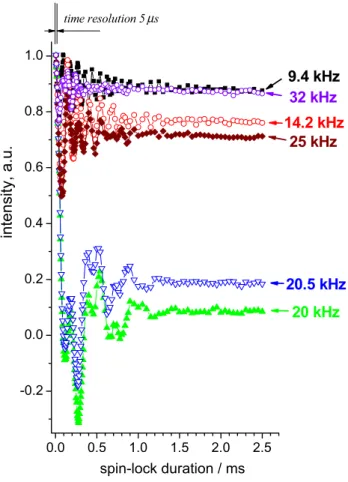
0.0 0.5 1.0 1.5 2.0 2.5 -0.2 0.0 0.2 0.4 0.6 0.8 1.0 14.2 kHz 32 kHz spin-lock duration / ms 9.4 kHz 25 kHz 20.5 kHz 20 kHz time resolution 5 s intensity, a.u. µ
Fig. 3 Experimentally measured 15N R
1ρ-relaxation decays (initial
part) of the integral signal in GB1 protein at 20 kHz and different spin-lock fields as indicated. All decays were normalized to unity at the initial point at 5 μs
0 1 2 3 4 0.6 0.7 0.8 0.9 1.0 spin-lock duration / ms intensity, a.u.
Fig. 4 Simulated R1ρ decays for the 15N–1H pair undergoing two-site
jumps at a single spin-lock field of 31.5 kHz (black line) and super-position of the decays simulated at B1-fields from 30 to 33 kHz with a
static solids, the decays are strongly multi-exponential; MAS causes a partial averaging of the dipolar couplings, which is still not complete, and the decays remain non-exponential although this is not always clearly seen in the experiments due to the insufficient signal-to-noise ratio. The exact shape of the relaxation decay cannot be calculated for a general case since it depends on the angular amplitude of motion.
For a quantitative analysis in terms of the motional corre-lation function, one usually employs a model-free approach or its modifications in order to estimate a single relaxation
parameter from such a non-exponential relaxation decay. This can be done in two ways: one may define the mean relaxation time constant or the mean relaxation rate constant. The former is provided by fitting the whole decay using the single-exponential fitting function, while the latter is repre-sented by the initial slope of the decay (see Supp. Info to ref. Krushelnitsky et al. 2014), as demonstrated in Fig. 8. While both procedures are mathematically correct, only the mean relaxation rate constant has a physical meaning, as shown a long time ago (Kalk and Berendsen 1976). The relaxation rate constant is directly proportional to the spectral density function R1,1ρ ~ J(ω), hence the mean relaxation rate
con-stant is proportional to the mean spectral density function: <R1,1ρ> ~ <J(ω)>. This is not the case for the mean relaxa-tion time constant. The correlarelaxa-tion funcrelaxa-tion obtained from the analysis of the initial slope of the relaxation decays is formally identical to that obtained from solution-state relax-ation times analyses (Torchia and Szabo 1982).
Although these issues have been known for a long time, solid-state relaxation decays have often been analyzed in terms of mean relaxation time (not rate) constants, which in some cases may lead to incorrect conclusions, one of such examples is described in (Smith et al. 2018).
Practically, the initial slope can be determined from fit-ting the decay with a sum of few exponential functions or using any phenomenological distribution function for the relaxation rates. From such fittings, the mean relaxation rate can be readily defined. According to our experience, fitting functions with a minimal number of independent param-eters such as a double exponential (two R1ρ, one relative amplitude, amplitude normalization coefficient) or a decay 5 10 15 20 25 30 35 40 45 0.0 0.2 0.4 0.6 0.8 1.0 -35 -30 -25 -20 -15 -10 -5 0 0.0 0.2 0.4 0.6 0.8 1.0
intensity, a.u.
ν
SL/ kHz
(
ν
SL-
ν
MAS) / kHz
A
νMAS = 20 kHz νMAS = 40 kHzB
Fig. 5 a Experimental (solid circles) and simulation (open triangles)
amplitude of the relaxation decay at 20 kHz MAS as a function of the spin-lock field. The experimental dependence was arbitrarily normal-ized in order to get a coincidence with the simulation dependence at low spin-lock fields. b The amplitudes of the relaxation signal
simu-lated at MAS rates 20 and 40 kHz plotted as a function of the differ-ence between the spin-lock and MAS frequencies. Experiments were conducted with the GB1 sample. For the simulations, the model of 2º-jumps with the jump rate 5000 s−1 was used
0 10 20 30 40 50 0.5 0.6 0.7 0.8 0.9 1.0 intensity, a.u. spin-lock duration / ms N N N H spin-lock 10 kHz 9 kHz 10 kHz N H
Fig. 6 Three R1ρ decays simulated for 20 kHz MAS, different
spin-lock fields and different spin systems (indicated in the figure). 15N–1H
distance in both cases was 1.02 Å, 15N–15N distances in 4-spins
struc-ture was 2.8 Å, which corresponds to the typical distance between backbone nitrogen atoms of neighbouring residues in a protein. In all cases two-site jumps of the 15N–1H bond with angular amplitude 5°
based upon a single-mode log-normal rate distribution (one median R1ρ, one distribution width parameter, amplitude
normalization coefficient) are sufficient practically in all cases (Roos et al. 2015). Some practical hints for the proper analysis of non-exponential decays are described in ESM.
It must be mentioned that in the case of the R1ρ
experi-ments, the initial slope of the decays is not seen due to the initial oscillations considered above, i.e. “dead time”. At the moment we are not in a position to suggest a truly robust and reliable way to decompose oscillations and relaxation contributions at the beginning of the decay. Thus, the correct quantitative analysis of the non-exponential R1ρ decays is
only possible when the “dead time” is considerably shorter than the inverse value of the relaxation rate, enabling a stable minimal-parameter fit as discussed above at times beyond the dead time.
Whole‑protein rocking motion
The 1D-integral experiments discussed above do not allow obtaining detailed site-specific information on slow con-formational protein dynamics. On the other hand, there is a kind of molecular motion for which the site-specific spectral resolution is not critical, which is the overall rock-ing motion of proteins in a solid environment, as reported recently both experimentally and computationally (Ma et al.
2015; Lamley et al. 2015b; Kurauskas et al. 2017). Such a global process assumes that all parts of a protein undergo the same motion and the correlation functions of all N–H bonds have a component with the same correlation time. The parameters of this common component can be obtained from 1D experiments and site-specific resolution for this is not necessary. The amplitude of this overall motion for dif-ferent N–H bonds can be however difdif-ferent. For example, if the rocking motion is a restricted rotation around an axis then the amplitude (order parameter) depends on the angle between this axis and N–H bond. Thus, the rocking motion amplitude obtained from 1D experiments is a mean ampli-tude over all N–H bonds. As discussed below, the overall motion in general case can be overlapped with the internal conformational motion that has similar time scale. In this case, the unambiguous discrimination between these two
Fig. 7 Typical examples of experimental (a) and simulated (b) R1ρ decays on a
semi-logarithmic scale. Dashed red lines indicate single-exponen-tial decays for comparison. Experiment: SH3 sample, MAS 20 kHz, spin-lock field 15 kHz; simulations: jump amplitude 20°, rate 500 s−1 0 10 20 30 40 50 0.4 0.5 0.6 0.7 0.8 0.9 1 0 10 20 30 40 0.3 0.4 0.5 0.6 0.7 0.8 0.9 1
intensity, a.u.
spin-lock duration / msA
B
mean relaxation rate constant Log (INTENSITY ) TIMEmean relaxation time constant
Fig. 8 Schematic presentation of the multi-exponential experimental relaxation decay (circles), initial slope (dashed line) and fitting the whole decay using a single-exponential function (red solid line)
types of molecular mobility from 1D data is impossible and site-specific measurements are necessary.
Previous analyses have shown that protein rocking occurs on the microsecond timescale (Lamley et al. 2015b; Kuraus-kas et al. 2017), thus near-rotary-resonance R1ρ measure-ments should provide critically important information on the parameters of the rocking motion. In this part of the work we apply 15N R
1ρ experiments for a comparative study of the
rocking motion in a set of four different solid protein sam-ples, taking into account all the methodological problems discussed above. Since in all four cases the experiments and the data analyses were performed in the same manner, the results can be compared directly.
Interpreting relaxation measurements in terms of molecu-lar motion is generally challenged by the fact that the spec-tral density function is sampled usually only at few frequen-cies. When only small number of relaxation parameters are measured, the fitted time constants and amplitudes may be subject to a large uncertainty (Smith et al. 2017). To resolve, at least partially, these ambiguities in determining motional time scales, we use relaxation measurements at multiple temperatures. Even when measured within a narrow tem-perature range, the temtem-perature dependence of a relaxation rate, i.e. its slope—even the sign of the slope (positive or negative)—is very informative for the determination of the motional correlation time. Varying both the RF field strength and the temperature and analysing all the data simultane-ously renders the set of the relaxation data effectively “two-dimensional”, which significantly improves the accuracy and precision of the fit results. The 1D approach allowed
the collection of such an extensive data set at multiple RF field strengths, three different temperatures and four different protein samples.
Below we present the analysis of the R1ρ rates measured at a wide range of differences (ωMAS − ωSL) and at three temperatures for each sample. The range of temperatures was limited so that the proteins remain native and that the microcrystalline samples would not freeze. In addition to
R1ρ’s, we also measured R1’s at the same temperatures. R1’s are not useful for studying rocking motions since these relaxation rates are sensitive to much faster dynamics. At the same time, while fitting the data we need to take into account faster motions as well since without knowledge of the amplitude of the fast motions, the order parameter of the rocking motion cannot be determined precisely.
Figure 9 presents typical examples of the R1ρ relaxation decays measured at different spin-lock frequencies. Simi-lar decays for one of the ubiquitin samples measured at 40 kHz are shown in ESM, Figs. S1 and S2. Even without any numerical analysis it is clearly seen that the relaxation becomes faster upon approaching spin-lock frequency to the MAS frequency. This is an unambiguous indication of the fact that the protein undergoes dynamics on the micro-second timescale, otherwise the R1ρ versus (ωMAS − ωSL) dependence would be flat (Krushelnitsky et al. 2014; Ma et al. 2014).
The initial oscillations were excluded from the analysis and the fitting was performed over all points beyond 3.5 ms spin-lock pulse duration. Figure 10 shows the result of the fitting of a typical relaxation decay using mono- and
Fig. 9 Experimental R1ρ decays
measured for GB1 at 21.5 °C and 20 kHz MAS for five different spin-lock fields as indicated (a). The panel b is a zoomed region indicated by the rectangle in the panel a. All decays were normalized to unity by the point at 3.5 ms (“dead time”), where the initial oscilla-tions have practically vanished. The experimental error can be assessed from the scatter of the points in the decays
0.01 0.1 1 10 100 -1.0 -0.5 0.0 0.5 1.0 1.5 2.0 2.5 3.0 3.5 4.0 4.5 5.0 spin-lock duration / ms 8 kHz 12 kHz 15 kHz 17 kHz 18 kHz Spin-lock frequencies: 0 10 20 30 40 50 0.7 0.75 0.8 0.85 0.9 0.95 1 spin-lock duration / ms 3.5 ms intensit y, a.u.
A
B
bi-exponential fitting functions. This is merely a demonstra-tion of the difference between the meaningless mean relaxa-tion time (from the single-exponential fit) and the physically relevant mean relaxation rate (see above) using a typical experimental relaxation decay. The non-exponential shape of the decays is barely seen, tempting one to neglect the non-exponentiality and to fit the decay with a single exponential. However, as it is shown in the figure, the values of the mean time and the mean rate are appreciably different.
After determining the set of the relaxation rates for all samples, one has to fit the data using a specific motional model. We suggest using a model with two motional modes—fast internal conformational motion on the nano-second timescale and slow overall protein rocking motion. Since we analyse the overall signal from the whole protein, we introduce a distribution of correlation times of the fast internal motion that takes into account the internal dynamic heterogeneity of a protein. Thus, a spectral density function reads
where S2
f ,S and 𝜏f ,S are the order parameters and the correla-tion times of the fast and slow mocorrela-tions, respectively;
(2) J(𝜔) = (1 − S2f) ∞ ∫ 0 𝜌(𝜏, 𝜏f, 𝛽) 𝜏 1 + (𝜔𝜏)2d𝜏 + S 2 f(1 − S 2 S) 𝜏S 1 + (𝜔𝜏S) 2
𝜌(𝜏, 𝜏f, 𝛽) is the distribution function that is parameterized
by two parameters—𝜏f , the centre of the distribution and β, the distribution width parameter. Without a distribution of the correlation times for the fast motion, good data fitting was unachievable. As for the distribution of the fast-motion correlation times, we used two phenomenological models, a log-normal and a modified non-symmetric Fuoss-Kirkwood distribution (Schneider 1991), for details see the ESM. The analysis assumes that the order parameters and the shape of the distribution function are the same at all temperatures. While in reality these are obviously temperature-dependent, the temperature dependence is likely rather weak, otherwise the proteins and crystals would not be rigid and stable. Tak-ing the temperature dependence of these parameters by some phenomenological function into account is in principle pos-sible, but this would make the fitting less certain and in any case would not lead to any significant change of the final results.
The slow (rocking) motion likely has a distribution of correlation times that can be caused either by inhomogeneity of a sample (e.g. defects in crystal packing) or an intrinsi-cally complicated shape of the rocking-motion correlation function arising from a possible inter-correlation of motion of neighbouring proteins in a crystal. We tried to fit the data assuming a distribution for the slow motion as well. How-ever, in all cases the inclusion of one more fitting parameter (distribution width for the slow-motion correlation times) leads to a practically negligible improvement of the fitting quality (results not shown). At the same time, the depend-ence of the main parameters of the slow motion, the cor-relation time and the order parameter, on the width of the distribution is rather weak. Thus, following the principle of Occam’s razor, we include in the fitting model only a single correlation time of the slow rocking motion.
As expected, the type of the distribution function has an effect on the parameters of the fast motion, but the slow-motion parameters are practically insensitive to it. Since we analyze the relaxation times at different temperatures, we assume an Arrhenius dependence of the correlation times on temperature,
where 𝜏20
f ,S are the correlation times at temperature 20 °C, and
Ef ,S are activation energies of the fast and slow motions.
Thus, the total number of fit parameters is seven: two order parameters, two correlation times, two activation energies (for the fast and slow motions) and the distribution width parameter for the fast motion. At the same time, the number of experimental points (relaxation rates) was 18–24 for each sample. Further details of the fitting procedure are laid out (3) 𝜏f ,S = 𝜏f ,S20⋅ exp (E f ,S R (1 T − 1 293K )) 0 10 20 30 40 50 0.7 0.75 0.8 0.85 0.9 0.95 1 spin-lock duration / ms intensity, a.u.
Fig. 10 A typical example of the R1ρ relaxation decay with barely
noticeable multi-exponentiality, measured on GB1 at 21.5 °C, 20 kHz MAS and a spin-lock field of 17 kHz. The dashed blue and solid red lines are single- and bi-exponential fits, respectively. The relaxation rates obtained from the single- and bi-exponen-tial fits are 6.5 ± 0.25 and 8.0 ± 1.0 s−1, respectively. In the
lat-ter case, the mean relaxation rate (i.e. initial slope) was obtained as ⟨R1𝜌⟩ = p⋅ R1𝜌a+ (1 − p) ⋅ R1𝜌b , where p and R1ρa,b are the relative
amplitude of one of the components and relaxation rate constants of two components of the decay, respectively (see Eqs. S1–S4 of ESM). The fitting values of these parameters are: p = 0.74 ± 0.5;
R1ρa=2.8 ± 5 s−1; R
in the ESM. The parameters of the fast motion may be poorly determined, since only R1 rate constants at a single
reso-nance frequency contain information on the fast dynamics, which is obviously not enough for a reliable determination of the nanosecond timescale part of the motional correlation function. Also, the activation energies are not determined very precisely since the temperature range of the experi-ments was quite narrow. Fortunately, the uncertainty of these parameters is a minor problem since the main goal of this work is to assess the timescale of the slow rocking motion and its order parameter, which could be reliably determined from the data since the abundant R1ρ rates sample the micro-second range of molecular dynamics in sufficient detail. All the fit parameters for two types of the distribution functions are presented in ESM, see Tables S1 and S2, and below in Table 1 we collect only the most important and relevant results—the order parameters and the correlation times of the slow rocking motion for the four different protein sam-ples. Table 1 also presents the angular amplitudes assuming the motional model to be jumps between two equivalent sites, which gives an impression of the angle of the whole protein reorientation on the microsecond time scale (this of course should not be necessarily the 2-site jumps). The last row in Table 1 is a solvent content in the protein crystals which will be discussed below. Figures 11 and 12 present the experimental relaxation rate constants and the fit curves.
The detection of slow motion in all crystals suggests, as mentioned above, the presence of an overall motional process, such as rigid-body rocking (Ma et al. 2015; Lam-ley et al. 2015b; Kurauskas et al. 2017). Alternatively, the observed very low amplitude of the slow motion in the non-selective experiment could also be explained by an internal conformational motion that affects only a (possibly rather small) fraction of residues. For the case of cubic-PEG-ub, the rigid-body nature of the motion has been confirmed by site-resolved measurements (Ma et al. 2015). For other pro-teins, especially revealing higher S2
S , the existence of the whole-body motion is so far not established. A criterion of such overall motion is a common component of the motional
correlation function with the same correlation time for all N–H bonds in a protein. To provide evidence for the global character of the motion, we performed site-resolved R1ρ
experiments in 2D-mode for the GB1 sample, i.e. the sample having the highest S2
S out of all four samples studied in the
Table 1 Order parameters, angular amplitudes (assuming 2-site jumps model) and the correlation times of the rocking motion at 20 °C for four samples
The numbers are averaged values of the fit results obtained using two different models for the τ-distribution functions for the fast motion (see Tables S1 and S2 in ESM for details). The solvent content in the crystals was determined using the molecular weight and unit cell parameters in the PDB entries 2GI9 (GB1), 1U06 (SH3), 3ONS (MPD-ub) and 3N30 (cubic-PEG-ub); the data for all these crystal structures have been col-lected at 100 K. Note that for a different crystal form of GB1, grown under very similar conditions (MPD, pH 4.5), corresponding to PDB entry 2QMT, the solvent content is also rather low, 45%, with a similar intermolecular β-sheet
GB1 SH3 Ubiq. MPD Ubiq. PEG
S2
S 0.9995 ± 0.00006 0.9915 ± 0.005 0.9965 ± 0.001 0.987 ± 0.003
Ang.ampl. 2-site jumps 1.5° 6.1° 3.9° 7.6°
𝜏S20/μs 41 ± 5 46 ± 4 30 ± 7 52 ± 7
Solvent content in crystal/% 33.6 49.8 49.6 56
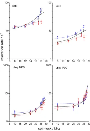
6 8 10 12 14 16 18 20 1 10 100 6 8 10 12 14 16 18 20 1 10 100 5 10 15 20 25 30 35 40 10 100 1000 5 10 15 20 25 30 35 40 10 100 1000 SH3 relaxation rate / s -1 GB1 ubiq. MPD spin-lock / kHz ubiq. PEG
Fig. 11 R1ρ relaxation rates as a function of spin-lock frequency for four different samples at three different temperatures. Circles—exper-imental data, solid lines—fitting curves. Blue dashed, black solid and red dotted lines correspond to the temperatures 13, 21.5 and 29 °C for SH3 and GB1 and 3, 15 and 27 °C for two ubiquitin samples, respec-tively
current work. Since collecting the large set of temperatures and RF field strengths that we covered by the 1D experi-ments would be too time consuming, we performed only two
R1ρ experiments at two spin-lock frequencies, 8 and 17 kHz, at a single temperature 21.5 °C. Having only two relaxation rate constants does not allow for any reliable quantitative estimation of the order parameters and correlation times, but the difference between the relaxation rates measured at two spin-lock fields unambiguously reveals the presence of μs motion. If the motion is faster or slower in comparison to a 10−6–10−4 s correlation time range, then the difference
is zero, otherwise the difference has an appreciable value proportional to the amplitude of the microsecond motion.
Figure 13 presents the relaxation rates R1ρ measured at
two spin-lock fields as well as their difference. In this analy-sis, we have only used arbitrary peak numbers, rather than residue numbers. The spectrum of our sample shown in Fig. S3 (ESM), obtained from similar crystallization conditions as previously reported ones (see “Materials and methods” section) differs from the previously published spectra to a point where unambiguous assignment of peaks to residues is possible only for 2–3 peaks. For the present analysis, the
assignment is not crucial, in particular as we find indeed a very similar behaviour for all residues.
Except for one peak (labelled as peak no. 6), all resi-dues reveal a positive difference, R1ρ(17 kHz)—R1ρ(8 kHz),
which indicates that all parts of the protein undergo the same type of motion on the μs timescale. Although the error bars in Fig. 13b are rather large, the decays themselves, even without the analysis, leave no doubt about the uniform R1ρ
spin-lock frequency dependence, see Fig. S4 (ESM). The absolute value of this difference for the majority of peaks is very similar, around 5 ± 2 s−1, which is in good
agree-ment with the corresponding value from the 1D relaxation experiment, 4.3 s−1 (Fig. 11). This finding fits much better
to the overall protein rocking motion rather than internal conformational dynamics since in the latter case only a part of residues would reveal such a dependence of R1ρ on the
frequency difference ωMAS − ωSL.
Several residues in the protein have elevated relaxation rates in comparison to the mean level, e.g. those correspond-ing to the peak numbers 3, 4, 5,12, 14, 15, 43, 47 and few others (Fig. 13a). These residues obviously undergo μs time scale motion and this motion is attributed to the internal conformational dynamics since only a small portion of resi-dues reveal such a behaviour. This motion for most peaks is however much faster (the correlation time presumably around 1 μs or shorter) than the overall rocking motion
0 5 10 15 20 25 30 35 0.1 1 GB1 ubiq. MPD relaxation rate / s -1
T /
oC
SH3 ubiq. PEGFig. 12 R1 relaxation rates as a function of temperature for four dif-ferent samples as marked. Circles—experimental data, solid lines— fitting curves 0 5 10 15 20 25 30 35 40 45 50 0 10 20 30 40 50 0 5 10 15 20 25 30 35 40 45 50 -5 0 5 10 15 20 R1ρ / s -1 8 kHz 17 kHz spin-lock frequency A peak number ∆ R1ρ / s -1 B
Fig. 13 Relaxation rates for different peaks in 2D-spectrum measured
in GB1 at 21.5 °C and MAS 20 kHz with spin-lock frequencies of 8 and 17 kHz (a), and difference R1ρ(17 kHz)–R1ρ(8 kHz) (b), both
plotted vs the peak number (which does not correspond to the pri-mary structure of the protein)
observed in the 1D experiments because the R1ρ difference (Fig. 13b) reveals no correlation with the absolute values of the relaxation rates. It follows from the fact that R1ρ versus
(ωMAS − ωSL) dependence for the motions with a correlation
time around 1 μs and shorter is flat, see Fig. 1 in (Krushelnit-sky et al. 2014). Thus, this internal motion does not contrib-ute to the rocking motion parameters obtained from the 1D data. The only exception is the peak no. 43: for this signal, the elevated rates reveal also the elevated difference between the rates, which indicates an additional internal motion with a correlation time of the order of (ωMAS − ωSL)−1.
We need to admit that the available 2D data do not prove that there are no additional internal conformational motion with a correlation time around 30–50 μs, i.e. the motion that undergoes only a part of residues in the protein. The accuracy of these data is rather low and probably this hypo-thetical motion is “hidden” within the error bars in Fig. 13. If this is true, the rocking motion amplitude has a contribution from this internal motion. On the other hand, the 2D data demonstrate that all the protein structure is dynamic on the μs timescale, and that the level of this mobility is roughly the same across the different parts of the protein. At the same time, the presence of the overall rocking motion does not necessarily mean that the protein itself remains fully rigid on the μs timescale. The rocking motion is possibly associ-ated with a bend or a twist of the whole structure, and thus discriminating between the whole protein reorientation and global structural plasticity is not a simple problem. Thus, the term “rocking motion” in some cases may imply rather some global dynamics than the restricted rigid body rotation only. Based on the analysis of MD simulations and NMR data, it has been suggested that local microsecond motion may be coupled to overall rocking motion (Kurauskas et al. 2017). Specifically, the reorientation of molecules within the crys-tal lattice is accompanied by the breaking and formation of a different set of inter-molecular interactions, which likely influence also the interconversion of different internal local conformations. Nonetheless, while we cannot exclude the presence of additional local motions having a correlation time close to that of global protein rocking, the uniformity of the R1ρ(17 kHz)–R1ρ(8 kHz) difference strongly suggests an overall/global motion, even for an order parameter as high as 0.9995.
As a further support for the global character of the detected motion, the two ubiquitin samples used in this study have previously been studied in a site-resolved manner, and, similarly to the case of GB1, a RF-field dependence of R1ρ
has been observed over all residues in the cubic-PEG-ub sample (Kurauskas et al. 2017). A global fit of the site-spe-cific near-rotary-resonance R1ρ relaxation dispersion profiles
of 22 available well-resolved amide sites in cubic-PEG-ub had been performed, and the obtained motional time con-stant was in the range of tens of microseconds, which is
in excellent agreement with the value found in the present study. The motional amplitude had previously been esti-mated to be ca. 3°–5°, corresponding to an order parameter ca. 0.98. Independent MD simulations had estimated an order parameter of overall rocking motion of ca 0.95–0.98. These values are also in a satisfactory agreement with the value found here, S2 = 0.987.
The availability data of four different protein crystals pro-vides interesting insight into the nature of rocking motion and allows us to suggest an explanation why the rocking motion amplitudes in these samples are so different, vary-ing by a factor of 5 when expressed as an effective rockvary-ing- rocking-motion angle. The solvent content of these crystals varies from 33% (GB1) to 56% (cubic-PEG-ub), see Table 1, with a good qualitative correlation with the amplitude of the rock-ing motion. For the case of GB1, which shows the lowest-amplitude overall motion, it is interesting to note that the proteins form inter-molecular β-sheets, extending through the entire crystal, with three NH···O=C hydrogen bonds con-necting the outermost β-strands of neighbouring molecules, see Fig. S5 (ESM). This tight interaction and packing of neighbouring molecules obviously limits the slow overall motion, providing a plausible explanation for the observed low amplitude.
While the overall-rocking motion amplitude differs signif-icantly between the different protein crystals, the previously determined fast local motional amplitudes of NH bonds appear to be more similar for GB1 (Mollica et al. 2012), SH3 (Chevelkov et al. 2009) and ubiquitin (Haller and Schanda
2013; Ma et al. 2015). The observation that the local motion is less influenced by crystal packing is not surprising as it has been established that the internal motion amplitudes in proteins are dictated by the local density of the internal pro-tein structure (Halle 2002). Local structural density in a pro-tein and packing density of propro-tein globules in a crystal of course should not be necessarily correlated, however, in both cases they seem to be a crucial factor affecting the amplitude of the fast internal and slow overall motions, respectively.
Despite the very different rocking amplitudes, the time scales for all samples are rather uniform from ca. 30 to 50 µs, without correlation to the amplitude. While we can only speculate about the origins of this similarity of time scales, this observation may indicate that the rocking motion is not a diffusive but rather a jump-like process. For a restricted dif-fusive motional model, e.g. wobbling in a cone or rotational diffusion around an axis, the apparent correlation time would be dependent on the amplitude of motion, assuming that the diffusion coefficient is the same. Such a dependence has been observed e.g. in numerical simulations of the motional correlation function in the Supporting Information to ref. (Zinkevich et al. 2013). For jumps between a small number of sites, the correlation time does not depend on the ampli-tude. Thus, the rocking motion is likely a jump-like process
between different molecular orientations. These different orientations or protein molecules in the crystal certainly differ in the pattern of inter-molecular interactions. Indeed, long MD simulation of different ubiquitin crystals with up to 48 molecules have revealed a pattern of fluctuating inter-molecular salt bridges and hydrogen bonds, and have sug-gested that different orientational states of the protein are stabilized each by a different set of interactions (Kurauskas et al. 2017). Thus, each set of interactions defines a certain energy minimum (a certain protein orientation). However, we are not yet sure that the life time of these inter-molec-ular interactions and hence, the overall-motion time scale is a universal value for all protein crystals, this obviously requires further experimental evidences.
Lastly, we note that the very high order parameter of the rocking motion can be not only the result of a small angular amplitude between similarly populated states, but could also be due to skewed populations of states which have a larger difference in their relative orientations. Previously observed high order parameters of the microsecond motion in SH3 were ascribed to a concept of low-populated (excited) states that implies jumps between conformational states with non-equal probabilities (Zinkevich et al. 2013). We now think that this microsecond motion is not internal but overall rock-ing motion, still the latter can be associated with the jumps between non-equal probability states. However, the available data do not allow making definite conclusions on this issue.
Conclusions
In this work we explored the capabilities and practical limi-tations of studying slow molecular motions by means of 15N R1ρ experiments in the vicinity of the rotary resonance con-ditions. A small difference between the spin-lock and MAS frequencies allows expanding the frequency range of the sampled molecular motions towards rather low frequencies. At the same time, practical problems should be properly han-dled while conducting the experiments. The most important methodological issues are as follows.
(a) Upon approaching to the rotary resonance condition, the amplitude of the useful relaxation signal decreases significantly. Consequently, one should seek a compro-mise between a small difference between spin-lock and MAS frequencies (if the slow dynamics is the target of study) and acceptable signal to noise ratio. When performing a series of measurements at different spin-lock RF field strengths, the measurement time may be distributed such that the sensitivity drop at near-rotary-resonance conditions is compensated. If the signal is very strong and sensitivity is not a limiting factor, then one should keep the ωMAS − ωSL difference at least
somewhat larger than the width of νSL-distribution due to B1-field inhomogeneity. Otherwise, the quantitative
analysis of the relaxation data would be too uncertain. (b) During the first few milliseconds of the R1ρ decay, the
useful relaxation signal is subject to initial coherent oscillations. The proper analysis of these oscillations is complex and difficult, and we suggest to consider this initial part of the decay as an effective “dead time” and not to include it in the analysis.
(c) One should avoid not only rotary resonance but also HORROR (ωSL = ωMAS/2) conditions. Homonuclear
15N–15N interaction in proteins is weak, but it is still
capable of distorting the relaxation decays significantly. This distortion is even more difficult to handle because of its low frequency, thus precluding simple time aver-aging; it thus affects the apparent initial decay rate the is the most relevant quantity.
(d) R1 and R1ρ relaxation decays in solids are always
non-exponential. Quite often this non-exponentiality is hardly seen in experiments, still, the decays are non-exponential. For correct quantitative analysis of the relaxation data in terms of the correlation function for-malism, one needs to determine not the mean relaxation time but the mean relaxation rate, the latter being the initial slope of the relaxation decay.
Making use of the fact that the 1D mode of the relaxation experiments allows much faster measurement, multiple 15N R1ρ’s at different spin-lock frequencies and temperatures were measured for four different microcrystalline protein samples in order to determine the parameters of the over-all rocking motion. The results show that the correlation time of the rocking motion is almost the same for all sam-ples (30–50 μs), however, the amplitudes are very different. The absolute values of the order parameter of the rocking motion are rather high; the most rigid protein, GB1, has an order parameter of 0.9995. The R1ρ experiments at two different spin-lock fields performed for this sample in 2D mode show that the very small amplitude corresponds to the overall motion of the whole protein, not internal conforma-tional dynamics of only a (possibly small) part of the protein structure. Thus, the rocking motion seems to be a general feature of proteins in a crystal. The rocking motion ampli-tude of the four samples correlates with the solvent content in the protein crystal suggesting that the amplitude depends on the packing density of a protein crystal. There are indica-tions that the rocking motion is likely a jump-like dynamic process, this however should be confirmed in future studies.
Acknowledgements The authors are grateful to Prof. Matthias Ernst for very useful and stimulating discussions in the course of the prepara-tion of this work. Prof. Bernd Reif is thanked for his support in prepa-ration of the SH3 sample. The authors acknowledge the funding from the Deutsche Forschungsgemeinschaft (DFG), collaborative research
center SFB TRR 102 (project A08), and the European Research Coun-cil (ERC-StG-311318). This work used the platforms of the Grenoble Instruct Center (ISBG; UMS 3518 CNRS-CEA-UJF-EMBL) with support from FRISBI INSB-05-02) and GRAL (ANR-10-LABX-49-01) within the Grenoble Partnership for Structural Biology (PSB).
Open Access This article is distributed under the terms of the
Crea-tive Commons Attribution 4.0 International License (http://creat iveco mmons .org/licen ses/by/4.0/), which permits unrestricted use, distribu-tion, and reproduction in any medium, provided you give appropriate credit to the original author(s) and the source, provide a link to the Creative Commons license, and indicate if changes were made.
References
Chevelkov V, Rehbein K, Diehl A, Reif B (2006) Ultrahigh resolution in proton solid-state NMR spectroscopy at high levels of deutera-tion. Angew Chem 45:3878–3881
Chevelkov V, Fink U, Reif B (2009) Accurate determination of order parameters from 1H, 15N dipolar couplings in MAS solid-state
NMR experiments. J Am Chem Soc 131:14018–14022 Franks WT, Zhou DH, Wylie BJ, Money BG, Graesser DT,
Fre-ricks HL, Sahota G, Rienstra CM (2005) Magic-angle spin-ning solid-state NMR spectroscopy of the β1 immunoglobu-lin binding domain of protein G (GB1): 15N and 13C chemical
shift assignments and conformational analysis. J Am Chem Soc 127:12291–12305
Gauto DF, Hessel A, Rovo P, Kurauskas V, Linser R, Schanda P (2017) Protein conformational dynamics studied by 15N and 1H R
1ρ
relax-ation dispersion: applicrelax-ation to wild-type and G53A ubiquitin crystals. Sol State Nucl Magn Reson 87:89–95
Giraud N, Blackledge M, Goldman M, Böckmann A, Lesage A, Penin F, Emsley L (2005) Quantitative analysis of backbone dynamics in a crystalline protein from nitrogen-15 spin–lattice relaxation. J Am Chem Soc 127:18190–18201
Good DB, Wang S, Ward ME, Struppe J, Brown LS, Lewandowski JR, Ladizhansky V (2014) Conformational dynamics of a seven trans-membrane helical protein anabaena sensory rhodopsin probed by solid-state NMR. J Am Chem Soc 136:2833–2842
Good D, Pham C, Jagas J, Lewandowski JR, Ladizhansky V (2017) Solid-state NMR provides evidence for small-amplitude slow domain motions in a multispanning transmembrane α-helical protein. J Am Chem Soc 139:9246–9258
Haeberlen U, Waugh JS (1969) Spin-lattice relaxation in periodically perturbed systems. Phys Rev 185:421–429
Halle B (2002) Flexibility and packing in proteins. Proc Nat Acad Sci USA 99:1274–1279
Haller JD, Schanda P (2013) Amplitudes and time scales of picosec-ond-to-microsecond motion in proteins studied by solid-state NMR: a critical evaluation of experimental approaches and appli-cation to crystalline ubiquitin. J Biomol NMR 57:263–280 Kalk A, Berendsen HJC (1976) Proton magnetic relaxation and spin
diffusion in proteins. J Magn Reson 24:343–366
Korzhnev DM, Kay LE (2008) Probing invisible, low-populated states of protein molecules by relaxation dispersion NMR spectroscopy: an application to protein folding. Acc Chem Res 41:442–451 Krushelnitsky A, Zinkevich T, Reichert D, Chevelkov V, Reif B (2010)
Microsecond time scale mobility in a solid protein as studied by the 15N R
1ρ site-specific NMR relaxation rates. J Am Chem Soc
132:11850–11853
Krushelnitsky A, Zinkevich T, Reif B, Saalwächter K (2014) Slow motions in microcrystalline proteins as observed by
MAS-dependent 15N rotating-frame NMR relaxation. J Magn
Reson 248:8–12
Kurauskas V, Weber E, Hessel A, Ayala I, Marion D, Schanda P (2016) Cross-correlated relaxation of dipolar coupling and chemical-shift anisotropy in magic-angle spinning R1ρ NMR measurements:
application to protein backbone dynamics measurements. J Phys Chem B 120:8905–8913
Kurauskas V, Izmailov SA, Rogacheva ON, Hessel A, Ayala I, Wood-house J, Shilova A, Xue Y, Yuwen T, Coquelle N, Colletier J-P, Skrynnikov NR, Schanda P (2017) Slow conformational exchange and overall rocking motion in ubiquitin protein crys-tals. Nat Commun 8:145
Kurbanov R, Zinkevich T, Krushelnitsky A (2011) The nuclear magnetic resonance relaxation data analysis in solids: general R1/R1ρ equations and the model-free approach. J Chem Phys
135:184104
Lakomek N-A, Penzel S, Lends A, Cadalbert R, Ernst M, Meier B (2017) Microsecond dynamics in ubiquitin probed by solid-state
15N NMR spectroscopy R
1ρ relaxation experiments under fast
MAS (60–110 kHz). Chem Eur J 23:9425–9433
Lamley JM, Lougher MJ, Sass HJ, Rogowski M, Grzesiek S, Lewan-dowski JR (2015a) Unraveling the complexity of protein backbone dynamics with combined 13C and 15N solid-state NMR relaxation
measurements. Phys Chem Chem Phys 17:21997–22008 Lamley JM, Oster C, Stevens RA, Lewandowski JR (2015b)
Inter-molecular interactions and protein dynamics by solid-state NMR spectroscopy. Angew Chem Int Ed 51:15374–15378
Levitt MH, Oas TG, Griffin RG (1988) Rotary resonance recoupling in heteronuclear spin pair systems. Isr J Chem 28:271–282 Ma P, Haller JD, Zajakala J, Macek P, Sivertsen AC, Willbold D,
Bois-bouvier J, Schanda P (2014) Probing transient conformational states of proteins by solid-state R1ρ relaxation-dispersion NMR spectroscopy. Angew Chem Int Ed 53:4312–4317
Ma P, Xue Y, Coquelle N, Haller JD, Yuwen Z, Ayala I, Mikhailovskii O, Willbold D, Colletier J-P, Skrynnikov NR, Schanda P (2015) Observing the overall rocking motion of a protein in a crystal. Nat Commun 6:8361
Mollica L, Baias M, Lewandowski JR, Wylie BJ, Sperling LJ, Rienstra SM, Emsley L, Blackledge M (2012) Atomic resolution structural dynamics in crystalline proteins from molecular simulation and NMR. J Phys Chem Lett 3:3657–3662
Mulder FAA, Mittermaier A, Hon B, Dahlquist FW, Kay LE (2001) Studying excited states of proteins by NMR spectroscopy. Nat Struct Biol 8:932–935
Nagashima H, Trebosc J, Lafon O, Pourpoint F, Paluch P, Potrzebowski MJ, Amoureux J-P (2017) Imaging the spatial distribution of radi-ofrequency field, sample and temperature in MAS NMR rotor. Solid State Nucl Magn Reson 87:137–142
Nielsen NC, Bildsoe H, Jakobsen HJ (1994) Double-quantum homonu-clear rotary resonance: efficient dipolar recovery in magic-angle spinning nuclear magnetic resonance. J Chem Phys 101:1805 Oas TG, Griffin RG, Levitt MH (1988) Rotary resonance recoupling
of dipolar interactions in solid-state magnetic resonance spectros-copy. J Chem Phys 89:692–695
Roos M, Hofmann M, Link S, Ott M, Balbach J, Rossler E, Saalwachter K, Krushelnitsky A (2015) The “long tail” of the protein tum-bling correlation function: observation by 1H NMR relaxometry
in a wide frequency and concentration range. J Biomol NMR 63:403–415
Saalwächter K, Fischbach I (2002) The application of MAS recou-pling methods in the intermediate motional regime. J Magn Reson 157:17–30
Saurel O, Iordanov I, Nars G, Demange P, Marchand TL, Andreas LB, Pintacuda G, Milon A (2017) Local and global fynamics in Klebsiella pneumoniae outer membrane protein a in lipid bilay-ers probed at atomic resolution. J Am Chem Soc 139:1590–1597
Schanda P, Ernst M (2016) Studying dynamics by magic-angle spin-ning solid-state NMR spectroscopy: principles and applications to biomolecules. Prog NMR Spectrosc 96:1–46
Schneider H (1991) Modified Fuoss-Kirkwood distribution function for interpretation of asymmetric NMR relaxation curves. J Polym Sci B 29:1171–1177
Smith AA, Testori E, Cadalbert R, Meier BH, Ernst M (2016) Char-acterization of fibril dynamics on three timescales by solid-state NMR. J Biomol NMR 65:171–191
Smith AA, Ernst M, Meier BH (2017) Because the light is better here: correlation-time analysis by NMR spectroscopy. Angew Chem Int Ed 129:13778–13783
Smith AA, Testori E, Cadalbert R, Meier BH, Ernst M (2018) Correc-tion to: characterizaCorrec-tion of fibril dynamics on three timescales by solid-state NMR. J Biomol NMR 70:203
Torchia DA, Szabo A (1982) Spin-lattice relaxation in solids. J Magn Reson 49:107–121
Tosner Z, Purea A, Struppe JO, Wegner S, Engelke F, Glaser SJ, Reif B (2017) Radiofrequency fields in MAS solid state NMR probes. J Magn Reson 284:20–32
VanderHart DL, Garroway AN (1979) 13C NMR rotating frame
relax-ation in a solid with strongly coupled protons: polyethylene. J Chem Phys 71:2773–2787
Zinkevich T, Chevelkov V, Reif B, Saalwächter K, Krushelnitsky A (2013) Internal protein dynamics on ps to μs timescales as stud-ied by multi-frequency 15N solid-state NMR relaxation. J Biomol