HAL Id: hal-00295659
https://hal.archives-ouvertes.fr/hal-00295659
Submitted on 31 May 2005
HAL is a multi-disciplinary open access
archive for the deposit and dissemination of
sci-entific research documents, whether they are
pub-lished or not. The documents may come from
teaching and research institutions in France or
abroad, or from public or private research centers.
L’archive ouverte pluridisciplinaire HAL, est
destinée au dépôt et à la diffusion de documents
scientifiques de niveau recherche, publiés ou non,
émanant des établissements d’enseignement et de
recherche français ou étrangers, des laboratoires
publics ou privés.
on stratospheric ozone chemistry
A. Stenke, V. Grewe
To cite this version:
A. Stenke, V. Grewe. Simulation of stratospheric water vapor trends: impact on stratospheric ozone
chemistry. Atmospheric Chemistry and Physics, European Geosciences Union, 2005, 5 (5),
pp.1257-1272. �hal-00295659�
www.atmos-chem-phys.org/acp/5/1257/ SRef-ID: 1680-7324/acp/2005-5-1257 European Geosciences Union
Chemistry
and Physics
Simulation of stratospheric water vapor trends: impact on
stratospheric ozone chemistry
A. Stenke and V. Grewe
Deutsches Zentrum f¨ur Luft- und Raumfahrt (DLR), Institut f¨ur Physik der Atmosph¨are, Oberpfaffenhofen, 82230 Weßling, Germany
Received: 16 August 2004 – Published in Atmos. Chem. Phys. Discuss.: 14 October 2004 Revised: 7 February 2005 – Accepted: 16 April 2005 – Published: 31 May 2005
Abstract. A transient model simulation of the 40-year time
period 1960 to 1999 with the coupled climate-chemistry model (CCM) ECHAM4.L39(DLR)/CHEM shows a strato-spheric water vapor increase over the last two decades of 0.7 ppmv and, additionally, a short-term increase after ma-jor volcanic eruptions. Furthermore, a long-term decrease in global total ozone as well as a short-term ozone decline in the tropics after volcanic eruptions are modeled. In order to un-derstand the resulting effects of the water vapor changes on lower stratospheric ozone chemistry, different perturbation simulations were performed with the CCM ECHAM4.L39-(DLR)/CHEM feeding the water vapor perturbations only to the chemistry part. Two different long-term perturbations of lower stratospheric water vapor, +1 ppmv and +5 ppmv, and a short-term perturbation of +2 ppmv with an e-folding time of two months were applied. An additional stratospheric water vapor amount of 1 ppmv results in a 5–10% OH increase in the tropical lower stratosphere between 100 and 30 hPa. As a direct consequence of the OH increase the ozone destruc-tion by the HOx cycle becomes 6.4% more effective. Cou-pling processes between the HOx-family and the NOx/ClOx -family also affect the ozone destruction by other catalytic reaction cycles. The NOx cycle becomes 1.6% less effec-tive, whereas the effectiveness of the ClOx cycle is again slightly enhanced. A long-term water vapor increase does not only affect gas-phase chemistry, but also heterogeneous ozone chemistry in polar regions. The model results indicate an enhanced heterogeneous ozone depletion during antarc-tic spring due to a longer PSC existence period. In contrast, PSC formation in the northern hemisphere polar vortex and therefore heterogeneous ozone depletion during arctic spring are not affected by the water vapor increase, because of the less PSC activity. Finally, this study shows that 10% of the global total ozone decline in the transient model run can Correspondence to: A. Stenke
(andrea.stenke@dlr.de)
be explained by the modeled water vapor increase, but the simulated tropical ozone decrease after volcanic eruptions is caused dynamically rather than chemically.
1 Introduction
Water vapor in the upper troposphere (UT) and lower strato-sphere (LS) plays a key role in atmospheric chemistry. The oxidation of H2O and CH4by excited oxygen O(1D) is the primary source of hydrogen oxides (HOx=OH+HO2) (Reac-tions R1–R2, see Appendix), which are involved in important catalytic reaction cycles that control the production and de-struction of ozone in the LS. The importance of the catalytic HOx-cycles for the photochemistry of stratospheric O3has already been identified in 1950 by Bates and Nicolet. Ad-ditionally, OH is important for changing the partitioning of the nitrogen and the halogen family which are crucial for the O3removal in the stratosphere.
Several studies discussed an increase in stratospheric wa-ter vapor (e.g. Evans et al., 1998; Michelsen et al., 2000; Nedoluha et al., 1998; Rosenlof et al., 2001). For exam-ple, Rosenlof et al. (2001) combined ten different data sets between 1954 and 2000, and estimated a water vapor trend of +1%/yr. Several reasons like enhanced methane oxi-dation, increased aircraft emission in the LS, a warming of the tropical tropopause, volcanic eruptions and large-scale changes in stratospheric circulation and troposphere-stratosphere-exchange have been discussed, but the observed stratospheric water vapor increase is not yet understood (Evans et al., 1998, and references therein). In contrast, trop-ical tropopause temperatures have been found to decrease (Zhou et al., 2001).
Oltmans et al. (2000) analyzed 20 years of water vapor measurements with the NOAA Climate Monitoring and Di-agnostics Laboratory (CMDL) frostpoint hygrometer over Boulder, CO, and reported a +1%/yr (+0.05 ppmv/yr) trend
1980 1982 1984 1986 1988 1990 1992 1994 1996 1998 2000
Water vapor mixing ratio
8 2 6 4 2002 8 2 6 4
Fig. 1. Time series of individual water vapor soundings with the
CMDL frostpoint hygrometer between 24 and 26 km at Boulder, CO (black) (Oltmans et al., 2000), and of monthly mean water vapor mixing ratios from ECHAM4.L39(DLR)/CHEM at 40◦N, 20 hPa (red) (Dameris et al., 2005). The linear trend with the 95% confidence interval is 0.044±0.012 ppmv/yr for Boulder and 0.029±0.007 ppmv/yr for the model simulation.
in the LS. Figure 1 shows a comparison of this time se-ries with a corresponding water vapor time sese-ries from a transient model simulation with ECHAM4.L39(DLR)-/CHEM (Dameris et al., 2005). Over the 20 year pe-riod between 1980 and 1999 both time series show a pos-itive trend. However, over the 40 year period from 1960 to 1999 the model results do not show a sustained posi-tive trend (see Dameris et al., 2005, for further informa-tion). The water vapor trend over Boulder (24–26 km) is +0.044±0.012 ppmv/yr (Oltmans et al., 2000). The simu-lated water vapor trend is about 35% weaker, it amounts to +0.029±0.007 ppmv/yr (the given uncertainties are the 95% confidence intervals using the t-statistic). A current study of Randel et al. (2004) reports a great disparity between the Boulder dataset and HALOE satellite data near Boulder re-garding the decadal water vapor changes for the period 1992– 2002. For the period 1992–1996 both datasets show a reason-able agreement. After 1997 the Boulder balloon data further increase in time, while HALOE stays relatively constant, so that HALOE shows small or even negative water vapor trends in the LS for 1992–2002. However, after 2001 both datasets again show a good agreement with remarkably low and per-sistent water vapor anomalies. Taking into account the above mentioned uncertainties in stratospheric water vapor trends the magnitude of the modeled water vapor increase is compa-rable with observations. The modeled water vapor increase is mainly associated with a warming of the tropical tropopause, which is in contrast to the observations where water vapor changes and changes of the tropical tropopause temperature are apparently in disagreement, and to some extent (≈30%) with the methane increase.
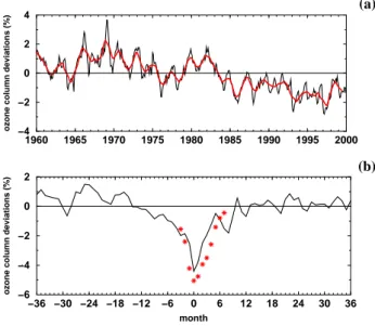
Furthermore, the transient model simulation shows a de-crease in global mean total ozone that is in agreement with observations (Fig. 2a, for further information see Dameris et al., 2005). Over the 20 year period between 1980 and 1999 the global mean ozone decline amounts approximately 1.7%/decade (5.5 DU/decade). Several studies have shown that increasing stratospheric water vapor affects the ozone
1960 1965 1970 1975 1980 1985 1990 1995 2000 −4 −2 0 2 4
ozone column deviations (%)
(a) −36 −30 −24 −18 −12 −6 0 6 12 18 24 30 36 month −6 −4 −2 0 2
ozone column deviations (%)
(b)
Fig. 2. (a) Modeled total ozone deviations, deseasonalized with
re-spect to the period 1979–1987 and expressed as percentages of the ground-based time average for the period 1964-1980, area-weighted mean 90◦N–90◦S (see Fioletov et al., 2002, for details of analysis). Red line shows a 13-month running mean. (b) Modeled total ozone deviations within the tropics (10◦N–10◦S) averaged over the last three major volcanic eruptions, expressed as percentages of the av-erage for the period 1964–1980. Month 0 indicates the minimum ozone value after the volcanic eruptions. The eruptions occurred between 8 and 23 months earlier. The red stars indicate the esti-mated reduction of the ozone column caused by the additional uplift during a volcanic period applying a linearized transport-chemistry column model.
budget significantly (e.g. Evans et al., 1998; Dvortsov and Solomon, 2001). One objective of this study is to assess the contribution of the simulated water vapor increase to the ana-lyzed ozone decrease in the above mentioned transient model simulation (Dameris et al., 2005).
Furthermore, the model simulation shows two pronounced water vapor peaks, associated with the eruption of the vol-canos El Chichon (17.33◦N, 93.20◦W) in 1982 and Mount Pinatubo (15.13◦N, 120.35◦E) in 1991 (Fig. 1). Enhanced water vapor mixing ratios are also seen in the Boulder dataset after the Pinatubo eruption in 1992 (Fig. 1). The heating ef-fect of additional volcanic aerosol on the tropical tropopause results in a short-term increase of stratospheric water vapor (Considine et al., 2001). In the model simulation the wa-ter vapor mixing ratios return to pre-volcanic levels approx-imately two years after the maximum value. Since both vol-canos are located in the tropics within the upwelling branch of the Brewer-Dobson circulation, it is expected that the gas-phase chemistry of the tropical LS is primarily influenced by a short-term increase in the water vapor loading. Figure 2b shows the simulated tropical ozone decline after the last three major volcanic eruptions. Beside the ozone trend analysis mentioned above a second major objective of this study is
to investigate whether these short-term ozone changes arise from a short-term water vapor increase.
In this paper we investigate the impact of stratospheric wa-ter vapor perturbations on ozone chemistry by model simula-tions with the coupled climate-chemistry model ECHAM4-.L39(DLR)/CHEM. We use a special method to prevent a feedback of the simulated water vapor increase to the model dynamics in order to separate the chemical effect. A short model description is given in the next section. Section 3 de-scribes the applied tracer approach. The results of our study are presented in Sects. 4.1 and 4.2, followed by a discussion in Sect. 4.3. A summary is given in the last section.
2 Model description
The coupled climate-chemistry model ECHAM4.L39(DLR)-/CHEM (Hein et al., 2001, hereafter referred to as E39/C) consists of the dynamic part ECHAM4.L39(DLR) (E39) and the chemistry module CHEM. E39 is a spectral general circu-lation model, based on the climate model ECHAM4 (Roeck-ner et al., 1996), and has a vertical resolution of 39 levels up to the top layer centered at 10 hPa (Land et al., 1999). A horizontal resolution of T30 (≈6◦isotropic resolution) is used in this study. The tracer transport, parameterizations of physical processes and the chemistry are calculated on the corresponding Gaussian transform grid with a grid size of 3.75◦×3.75◦. Water vapor, cloud water and chemical species are advected by a so-called semi-Lagrangian scheme.
The chemistry module CHEM (Steil et al., 1998) is based on the family concept. It includes stratospheric homoge-neous and heterogehomoge-neous ozone chemistry and the most rel-evant chemical processes for describing the tropospheric background NOx-CH4-CO-HOx-O3chemistry with 107 pho-tochemical reactions, 37 chemical species and 4 heteroge-neous reactions (R12–R15) on polar stratospheric clouds (PSCs) and on sulfate aerosols. CHEM does not yet consider bromine chemistry. Mixing ratios of methane (CH4), nitrous oxide (N2O) and carbon monoxide (CO) are prescribed at the surface following IPCC (2001) for the year 2000. Zon-ally averaged monthly mean concentrations of chlorofluo-rocarbons (CFCs) and upper boundary conditions for total chlorine and total nitrogen are taken from the 2-D model of Br¨uhl and Crutzen (1993). Nitrogen oxide emissions at the surface (natural and anthropogenic sources), from lightning and aircraft are considered. The model set-up follows Hein et al. (2001) except for the total amounts of emissions, light-ning NOx, which is parameterized according to Grewe et al. (2001), and a more detailed sulfate aerosol chemistry.
The model E39/C can be run in two different modes: with-and without-feedback. In the without-feedback mode the concentrations of the radiatively active gases H2O, O3, N2O, and CFCs calculated by CHEM do not feed back to the radia-tive scheme of E39. Prescribed climatological mixing ratios of the radiatively active gases are used as input for the
radia-tive scheme instead (Hein et al., 2001). Note that the tran-sient model simulation reported by Dameris et al. (2005), on the other hand, was integrated in the with-feedback mode in-cluding the chemical feedbacks on radiatively active gases. 2.1 Model climatology
The model climatology was extensively validated in Hein et al. (2001). Generally, the model offers a reasonable de-scription of dynamic and chemical processes and of the pa-rameter distributions in the troposphere and LS. In particular, the modeled dynamics in the northern hemisphere LS are in good agreement with observations. The model is able to re-produce the high interannual dynamic variability including the occurrence of stratospheric warmings. The subsidence of air masses inside the arctic polar vortex is also repro-duced by the model. However, Hein et al. (2001) have also mentioned some model weaknesses which seem to be linked to a cold temperature bias in the southern hemisphere polar stratosphere. This temperature bias leads to a too cold and too stable polar vortex and, therefore, influences the antarctic ozone chemistry. This “cold-pole” problem is often consid-ered as being an effect of the low model top at 10 hPa, but it should be mentioned that this problem is also present in a number of middle atmosphere models (e.g. Pawson et al., 2000). Sometimes, even the use of this kind of models for coupled chemistry-climate simulations is questioned (Austin et al., 1997). Nevertheless, the results of Hein et al. (2001) and further studies of Schnadt et al. (2002) show that CCMs with a model top centered at 10 hPa and an adequate verti-cal resolution in the UT/LS region are appropriate to inves-tigate chemistry-climate interactions in the LS. Furthermore, a recent inter-comparison of different CCMs by Austin et al. (2003) revealed that low top models reproduce the observed total ozone distribution as well as high top models. Possi-ble effects of the above mentioned model weaknesses on the results of our study will be discussed in the concluding dis-cussion.
2.1.1 Water vapor
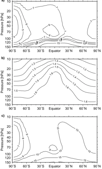
Figure 3 displays the modeled annual and zonal mean wa-ter vapor and methane mixing ratios as well as the zonal mean of the quantity 2×CH4+H2O. The modeled water vapor distribution shows a strong vertical gradient in the tropopause region following the vertical temperature gradi-ent. Minimum water vapor mixing ratios occur right above the tropical tropopause where the temperatures are lowest. Therefore, the model reproduces the observed water vapor distribution in the UT/LS region reasonably. However, the observed meridional water vapor gradient is not adequately represented in the model which is probably caused by numer-ical diffusion of the advection scheme. As already stated in Hein et al. (2001), modeled stratospheric water vapor mix-ing ratios are systematically higher than observed (see also
4 5 6 6 6 6 7 7 7 7 7 7 8 8 8 9 9 9 10 10 10 15 Pressure [hPa] 90˚S 60˚S 30˚S Equator 30˚N 60˚N 90˚N 150 120 100 70 50 40 30 20 10 a) 1.2 1.2 1.3 1.3 1.3 1.4 1.4 1.4 1.5 1.5 1.5 1.5 1.6 1.6 1.6 1.6 Pressure [hPa] 90˚S 60˚S 30˚S Equator 30˚N 60˚N 90˚N 150 120 100 70 50 40 30 20 10 b) 7 8 9 9 9 10 10 10 10 10 15 15 15 Pressure [hPa] 90˚S 60˚S 30˚S Equator 30˚N 60˚N 90˚N 150 120 100 70 50 40 30 20 10 c)
Fig. 3. Annual average of (a) zonal mean water vapor mixing
ra-tios (ppmv), (b) zonal mean methane mixing rara-tios (ppmv) and
(c) zonal mean 2×CH4+H2O (ppmv). Averaged over the last
10 years (1990–1999) of the transient model simulation (Dameris et al., 2005).
Fig. 1). A comparison between modeled temperatures and ECMWF reanalysis reveals a warm temperature bias near the model’s tropical tropopause (Land et al., 1999), which results in enhanced entry level mixing ratios [H2O]e (mod-eled: 5.9 ppmv, observed: 3.6–4.1 ppmv; SPARC, 2000). The southern polar stratosphere is characterized by strong dehydration in antarctic winter which is overestimated in the model. This behavior can be directly attributed to the too cold and too stable antarctic polar vortex (Hein et al., 2001). The modeled methane distribution is shown in Fig. 3b. In the tropics the methane mixing ratio decreases from about 1.65 ppmv to 1.2 ppmv near 10 hPa which is in good agree-ment with HALOE observations (Rosenlof, 2002). The meridional gradient of methane is slightly underestimated in
the model. As mentioned in Hein et al. (2001) this might be taken as an indication for an effect of the low upper bound-ary.
In order to exclude an upper boundary effect on the mod-eled water vapor distribution Fig. 3c shows the zonal mean mixing ratio of the quantity 2×CH4+H2O. The quan-tity 2×CH4+H2O should be nearly uniform throughout the stratosphere away from regions of dehydration in the winter polar vortex. The distribution of the quantity 2×CH4+H2O is dominated by the modeled water vapor distribution. Away from the southern polar region the distribution is nearly constant, whereas northern hemispheric values are slightly higher than in the southern hemisphere which is caused by the water vapor distribution. Figure 3c does not show a sub-stantial increase of the quantity 2×CH4+H2O towards the model top. Therefore, an upper boundary effect on the mod-eled water vapor is not expected.
2.1.2 Hydroxyl radical
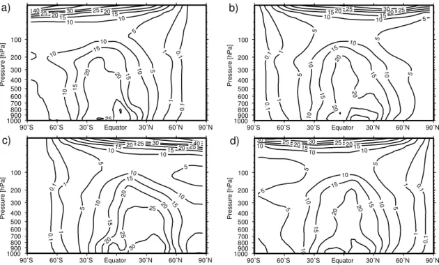
Since the hydroxyl radical (OH) plays a crucial role for the present study, possible model deficiencies have to be con-sidered. Figure 4 shows a vertical cross-section of the zon-ally and monthly averaged OH distribution in E39/C. Be-cause of the extreme variability of OH in time and space due to the high dependency on the solar zenith angle (Hanisco et al., 2001), in situ OH measurements are not appropri-ate for model evaluation. Spivakovsky et al. (2000) cal-culated a global climatological distribution of tropospheric OH (referred to OHSp hereafter) using observations of
pre-cursors for OH like O3, H2O, CO, hydrocarbons and NOt (defined as NO2+NO + 2N2O5+NO3+HNO2+HNO4, Spivakovsky et al., 2000) as well as observed temperatures and cloud optical depths as input for a photochemical box model. OHSp shows the highest zonal mean OH
con-centrations in the tropics at ca. 600 hPa, peaking at about 25×105molecules/cm3. Within this altitude range the trop-ical OH concentrations in E39/C are in good agreement with OHSp. The OH distribution in E39/C has its maximum
closer to the surface. This might be associated with the missing effects of non-methane-hydrocarbons (NMHCs) on OH in E39/C. OH is depleted over forested tropical conti-nents by the influence of NMHCs (Lawrence et al., 2001). In both OH distributions the maximum OH concentrations are shifted to the respective summer hemisphere during January and July, following the position of the sun. During April and October both OH distributions are mostly hemispher-ically symmetric. The mid-latitudes exhibit a strong sea-sonal cycle that is associated with sunlight and water vapor variations. Both OH distributions show very low OH con-centrations at high latitudes during winter. OHSp shows a
more pronounced vertical gradient between 500 and 100 hPa. Hence E39/C slightly overestimates the OH concentrations in this altitude range. Generally, the comparison of both
0.1 0.1 1 1 5 5 10 10 10 10 10 10 15 15 15 15 15 20 20 20 20 25 25 25 30 40 100 200 300 400 500 600 700 800 900 1000 Pressure [hPa] 90˚S 60˚S 30˚S Equator 30˚N 60˚N 90˚N 0.1 0.1 1 1 5 5 5 5 5 10 10 10 10 10 10 15 15 15 15 15 20 20 20 20 20 25 30 25 100 200 300 400 500 600 700 800 900 1000 Pressure [hPa] 90˚S 60˚S 30˚S Equator 30˚N 60˚N 90˚N 0.1 0.1 1 1 5 5 5 10 10 10 10 10 15 15 15 15 15 20 20 20 20 20 25 25 25 25 30 30 40 100 200 300 400 500 600 700 800 900 1000 Pressure [hPa] 90˚S 60˚S 30˚S Equator 30˚N 60˚N 90˚N 0.1 0.1 1 1 5 5 5 5 5 10 10 10 10 10 10 10 15 15 15 15 15 20 20 20 20 25 25 30 30 100 200 300 400 500 600 700 800 900 1000 Pressure [hPa] 90˚S 60˚S 30˚S Equator 30˚N 60˚N 90˚N a) b) c) d)
Fig. 4. Zonally and monthly averaged distribution of OH (105molecules/cm3) for January (a), April (b), July (c) and October (d) as modeled with E39/C. The figure shows a 10-year-climatology, 2000 climate.
Table 1. Overview of analyzed model experiments.
EXP feedback mode H2O perturbation simulation period
CNTL without feedback 0 ppmv, reference simulation 11 years
VOLC without feedback 2 ppmv, July and August, short-term increase 5 annual cycles July-June (last 5 years of CNTL) H2O 1 without feedback 1 ppmv, long-term increase 11 years
H2O 5 without feedback 5 ppmv, long-term increase 11 years
OH distributions shows that for the matter of this study the modeled OH distribution is realistically enough reproduced.
3 Methodology
3.1 Water vapor perturbations
Increasing stratospheric water vapor affects atmospheric dy-namics as well as the chemical composition of the atmo-sphere. Either effect contributes to a modified ozone distri-bution. In turn, the changed ozone distribution again affects atmospheric dynamics. For a better understanding of cou-pling processes between atmospheric chemistry and dynam-ics this study investigates the impact of an additional water vapor loading on stratospheric chemistry without changing atmospheric dynamics. Therefore, the model was run with-out feedback effects of the modeled water vapor increase on model dynamics. For this purpose a special tracer approach was introduced in E39/C: Two water vapor tracers are
dis-tinguished – the background water vapor and a water vapor perturbation. The radiative calculations are performed with the background water vapor and the model chemistry is com-puted with the “chemical” water vapor. The “chemical” wa-ter vapor field is defined as follows:
H2OChemistry=H2OBackground+H2OPerturbation
The water vapor perturbation is transported like an arbitrary tracer by the semi-Lagrangian advection scheme of E39/C. In order to treat the water vapor perturbation as realistic as possible it has to pass the same physical source and sink processes as the background water vapor. These processes include convection, condensation and vertical exchange by turbulence. This means, if cloud formation and precipitation cause a reduction of the background water vapor content by 10% within one model grid box, then the amount of the wa-ter vapor perturbation within this grid box is also reduced by 10%. The water vapor perturbation is fixed to a constant value within the tropical LS at each integration time step.
0.0 0.2 0.4 0.6 0.8 1.0 1.2 1.4 1.6 1.8 2.0
Jul Aug Sep Oct Nov Dec Jan Feb Mar Apr May Jun
89 hPa, 30˚N 89 hPa, 30˚S 0.0 0.1 0.2 0.3 0.4 0.5 0.6 0.7 0.8 0.9 1.0
Jul Aug Sep Oct Nov Dec Jan Feb Mar Apr May Jun
89 hPa, 60˚N 89 hPa, 60˚S
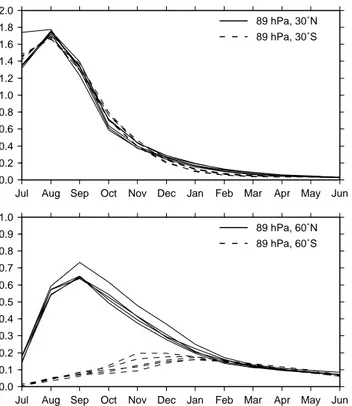
Fig. 5. Five annual cycles of the zonal mean water vapor
perturba-tion (ppmv) at 89 hPa, 30◦N/S (upper panel) and 60◦N/S (lower panel) of the simulation VOLC. Solid line: northern hemisphere; dashed line: southern hemisphere.
Below 200 hPa the perturbation field is set to zero since this study concentrates on the stratosphere.
3.2 Experimental design
For the current study various model simulations with E39/C were performed. A short overview of the performed simula-tions is given in Table 1. The model was run in the without-feedback mode. Thus, all experiments have identical meteo-rology. The adopted mixing ratios of greenhouse gases and NOx emissions of different sources represent atmospheric conditions of the year 2000 (Tables 2 and 3). The simu-lations CNTL, H2O 1 and H2O 5 were integrated over 11 years in a quasi-stationary state (time slice simulations). The last five years of the integration period were analyzed. The simulation CNTL was performed without a water vapor per-turbation as reference simulation. As mentioned above, this paper deals with two different objectives: 1. Chemical impact of a short-term increase of stratospheric water vapor after a volcanic eruption. Therefore, an ensemble of five 1-year-simulations was analyzed, representing the last five years of CNTL (hereafter referred to as VOLC). Each annual cycle starts in July, since the Mount Pinatubo eruption occurred 15 June 1991. During July and August additional water vapor is “emitted” in the tropical lower stratosphere by the above
Table 2. Mixing ratios of greenhouse gases adopted for the year
2000 as recommended by IPCC (2001).
CO2(ppmv) CH4(ppmv) N2O (ppbv) Cly(ppbv)
375 1.76 316 2.7
Table 3. NOxemissions adopted for the year 2000 (∗taking into
account IPCC, 2001, rates of increase). NOxsource Global source Reference
(Tg(N)/yr)
Air traffic 0.7 Schmitt and Brunner (1997)∗ Lightning ≈5 Grewe et al. (2001) Industry, Traffic 33.0 Benkovitz et al. (1996)∗ Soils 5.6 Yienger and Levy (1995)∗ Biomass burning 7.1 Hao et al. (1990)∗
mentioned method. The water vapor perturbation in the trop-ical LS is set to 2 ppmv. For the rest of the year the emis-sion is stopped. Five different years were chosen to cover a range of dynamical situations. Figure 5 shows the annual cycle of the water vapor perturbation for the five simulations at 89 hPa at 30◦N/S and 60◦N/S. Within the tropics the per-turbation shows a rapid decrease after the peak in August. The e-folding time of the perturbation is 2 months. The vari-ability within the ensemble of five 1-year-simulations is very small. At 30◦ the interhemispheric differences are just as little as the differences between the different annual cycles of VOLC. At 60◦the interhemispheric differences are much more pronounced. In the northern hemisphere the perturba-tion peaks in September whereas the southern hemispheric peak occurs 3 month delayed in December. This pattern indi-cates a more intense northward transport in the model within the lowermost stratosphere during summer. This transport pattern has also been identified by Grewe et al. (2004) who studied the impact of horizontal transport caused by stream-ers on the chemical composition of the tropopause region.
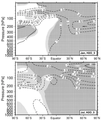
2. Chemical impact of a long-term stratospheric water va-por increase. For that purpose two long-term perturbation experiments were performed, H2O 1 and H2O 5. In H2O 5 the water vapor perturbation in the tropical LS is set to ca. 5 ppmv. This value corresponds roughly to a doubling of water vapor within the LS. This model experiment was designed as a maximum impact scenario. Taking into ac-count a stratospheric water vapor trend of +0.05 ppmv/yr the doubling of water vapor would be reached in ca. 100 years. The simulation H2O 1 was performed like H2O 5, but the perturbation was set to 1 ppmv. Figure 6 shows the clima-tological mean distribution of the water vapor perturbation in H2O 5 for January and July. The dark shaded area in-dicates the “source region” where the perturbation is fixed.
0.5 0.5 0.5 1 1 1 2 2 2 3 3 3 3 3 4 4 4 4.5 4.5 4.5 100 200 300 400 500 600 700 800 900 1000 Pressure [hPa] 90˚S 60˚S 30˚S Equator 30˚N 60˚N 90˚N Jan, H2O_5 0.5 0.5 0.5 1 1 1 2 2 2 2 3 3 43 4 4 4 4 4 4.5 4.5 4.5 100 200 300 400 500 600 700 800 900 1000 Pressure [hPa] 90˚S 60˚S 30˚S Equator 30˚N 60˚N 90˚N Jul, H2O_5
Fig. 6. Zonally averaged volume mixing ratio of the water vapor
perturbation (ppmv). This figure displays the mean over 5 analyzed years, simulation H2O 5. The gray-shaded area marks the tropical “source region” of the water vapor perturbation.
Approximately 70% of the tropical perturbation can be found around 70◦N (≈3.5 ppmv), whereas the perturbation is much lower around 70◦S (southern hemispheric values 15%–20%
lower than northern hemispheric values). Again, these results indicate a more intense northward transport. The antarctic winter stratosphere is characterized through strong dehydra-tion. The dehydration of the arctic winter stratosphere is less intensive. Generally, the results for simulation H2O 1 show the same pattern, just the absolute values are 5 times smaller.
4 Results
In this section the impact of a short-term increase of strato-spheric water vapor (Sect. 4.1) as well as two different long-term water vapor perturbations (Sect. 4.2) on stratospheric ozone chemistry are analyzed in detail. The description of chemical processes and reactions (see Appendix) is limited to those which are important for this study. A complete descrip-tion of stratospheric ozone chemistry can be found e.g. in Seinfeld and Pandis (1998).
0 0 0 0 0.5 0.5 0.5 0.5 0.5 1 1 1 1 3 3 5 5 7 -90 -60 -30 0 30 60 90 Latitude
Jul Aug Sep Oct Nov Dec Jan Feb Mar Apr May Jun
0 0 0 0.5 0.5 0.5 0.5 0.5 0.5 1 1 1 1 1 3 3 3 5 5 5 7 7 10 10 -90 -60 -30 0 30 60 90 Latitude
Jul Aug Sep Oct Nov Dec Jan Feb Mar Apr May Jun
15
Fig. 7. Relative changes (%) of zonal mean OH concentration at
50 hPa (upper panel) and 80 hPa (lower panel) depending on lati-tude and season, VOLC-CNTL/CNTL. Heavy (light) shaded areas indicate the 99% (95%) significance level of the displayed changes (t-test).
4.1 Short-term increase of stratospheric water vapor This section deals with the impact of a short-term increase of stratospheric water vapor as associated with strong volcanic eruptions like the Mount Pinatubo eruption in 1991 (simula-tion VOLC). It should be pronounced that the impact of the additional volcanic aerosol surface area on ozone chemistry is not taken into account.
Since water vapor is an important source of odd hydrogen (Reaction R1) the short-term water vapor increase results in an enhanced stratospheric OH concentration. Figure 7 shows the percentage changes of the OH concentration at 50 hPa (upper panel) and 80 hPa (lower panel) in the VOLC sim-ulation depending on latitude and season. The OH concen-tration increases in both hemispheres. The most pronounced changes occur within the tropics associated with the highest H2O perturbation. The tropical OH increase peaks with up to 15% at 80 hPa in July and with up to 7% at 50 hPa in August. The 50 hPa level is above the “source” region of the H2O perturbation (≈96–70 hPa). This indicates that the modeled upward transport within the tropics between 80 and 50 hPa takes about one month. Of special interest are the two peaks at ca. ±30–40◦at 80 hPa. This pattern is linked to the polwards and downwards transport of the maximum OH sig-nal. In contrast, at 50 hPa the maximum is located symmetri-cally around the equator. The changes within the polar win-ter regions are not relevant due to the low OH background concentrations.
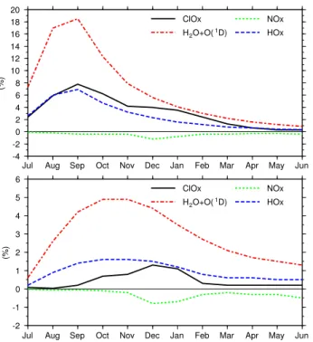
-4 -2 0 2 4 6 8 10 12 14 16 18 20 (%)
Jul Aug Sep Oct Nov Dec Jan Feb Mar Apr May Jun ClOx H2O+O(1D) NOx HOx -2 -1 0 1 2 3 4 5 6 (%)
Jul Aug Sep Oct Nov Dec Jan Feb Mar Apr May Jun ClOx
H2O+O(1D)
NOx HOx
Fig. 8. Percentage increase/decrease of different ozone destroying
cycles/reactions in VOLC compared to CNTL at 50 hPa. Upper panel: tropics, lower panel: sum of northern and southern mid-latitudes (45◦).
Changing stratospheric OH levels affect the different ozone destruction reactions. Figure 8 shows the rela-tive changes of the effecrela-tiveness of the HOx, ClOx and NOxcycle (Reactions R3 and R4) as well as of the reaction H2O + O(1D) → 2OH (removal of odd oxygen) at 50 hPa and different latitudes (upper panel: tropics, lower panel: mid-latitudes) caused by the stratospheric OH increase. The background contribution of the different processes to the ozone destruction in CNTL is given in the first row of Ta-ble 4, the relative changes of ozone loss rates for August and December are given in rows 3 and 4. The dominant ef-fect of higher water vapor concentrations is the increasing ozone destruction through the HOx cycle. Within the trop-ics the increase of the HOxcycle peaks in September with approximately 7% compared to CNTL. Additionally, the re-action H2O + O(1D) becomes more effective, but this reac-tion has only little importance. Enhanced HOx levels also change the catalytic effectiveness of ClOx and NOx cycle. On the one hand, chlorine activation is intensified through Reaction (R6). Reaction (R7) additionally benefits chlorine catalyzed ozone depletion in the LS. As displayed in Fig. 8 the ozone loss through the ClOx cycle is slightly intensi-fied. On the other hand, additional HOx tends to reduce ozone loss by the NOxcycle via Reaction (R5). However, the changes of the NOxcycle are negligible (≤−1%). Qualita-tively, the mid-latitudes show the same results as the tropics. The changes of the effectiveness are less pronounced than in
-10 -10 -7 -7 -7 -5 -5 -5 -5 -5 -3 -3 -1 -1 -1 0 0 0 0 -90 -60 -30 0 30 60 90 Latitude
Jul Aug Sep Oct Nov Dec Jan Feb Mar Apr May Jun
-5 -5
Fig. 9. Relative changes (0.01%) of zonal mean total ozone
de-pending on latitude and season, VOLC-CNTL/CNTL. Heavy (light) shaded areas indicate the 99% (95%) significance level of the dis-played changes (t-test).
the tropics since the OH increase is less. Additionally, the peaks are slightly shifted to November/December due to the transport times between tropics and mid-latitudes.
The changing ozone destruction yields a global reduction of total ozone except in tropical and mid-latitude regions dur-ing July as presented in Fig. 9. The short-term total ozone increase within the tropics during July is associated with an intensified oxidation of methane caused by the additional OH and the resultant increase in ozone production via Re-actions (R8)–(R11). This increased ozone production is re-stricted to the altitude range 100–80 hPa and compensates the enhanced effectiveness of the HOxcycle. The enhanced ozone production is to some extent counterbalanced by a more intensive NOx cycle, but the extra ozone production dominates. One month later the water vapor perturbation has also reached higher altitudes, where the ozone depletion by the HOxcycle becomes more important. Then, the enhanced ozone destruction by the HOxcycle overcompensates the in-creased ozone production at lower altitudes. Whether a trop-ical water vapor perturbation leads to ozone loss or ozone production depends on the relative contributions of the above mentioned mechanisms, which are dependent on pressure, latitude and season.
No results are shown for southern high latitudes during antarctic winter and spring in Fig. 9. Right after the initial-ization of the experiments the model results show an unreal-istic ClONO2increase at the upper boundary in the region of the polar vortex edge. Dynamical reasons for this ClONO2 increase are not possible, since the experiments CNTL and VOLC simulate identical meteorology. Chemical conversion between the individual members of the ClX-family caused by the OH increase is also very unlikely, since the changes of other chemical species like HCl or ClOxdo not show an adequate behavior. Numerical effects of the semi-Lagrangian advection scheme are the most probable explanation for this behavior. In some extreme cases the semi-Lagrangian ad-vection scheme may lead to a counter gradient vertical trans-port (Grewe et al., 2002). This problem is only present in
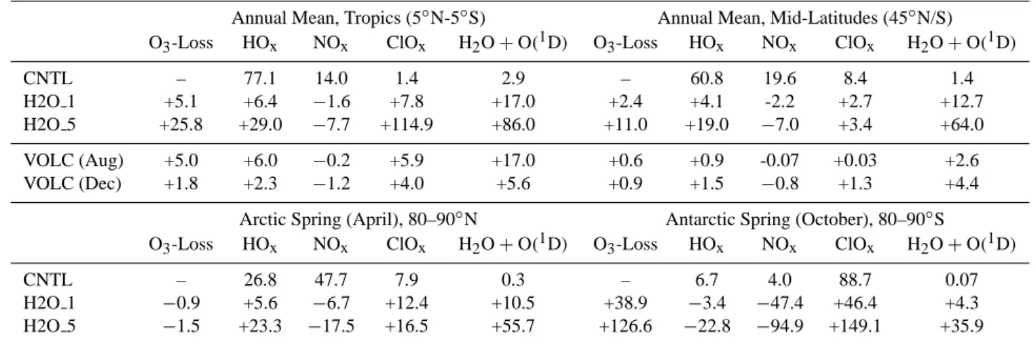
Table 4. Ozone destroying cycles/reactions at 50 hPa, different latitudes and seasons. CNTL: Contribution of each reaction to the total ozone
destruction [%]. VOLC, H2O 1 and H2O 5: Changes compared to CNTL [%]. The term O3-Loss includes all ozone destroying reactions
considered in E39/C.
Annual Mean, Tropics (5◦N-5◦S) Annual Mean, Mid-Latitudes (45◦N/S) O3-Loss HOx NOx ClOx H2O + O(1D) O3-Loss HOx NOx ClOx H2O + O(1D)
CNTL – 77.1 14.0 1.4 2.9 – 60.8 19.6 8.4 1.4 H2O 1 +5.1 +6.4 −1.6 +7.8 +17.0 +2.4 +4.1 -2.2 +2.7 +12.7 H2O 5 +25.8 +29.0 −7.7 +114.9 +86.0 +11.0 +19.0 −7.0 +3.4 +64.0 VOLC (Aug) +5.0 +6.0 −0.2 +5.9 +17.0 +0.6 +0.9 -0.07 +0.03 +2.6 VOLC (Dec) +1.8 +2.3 −1.2 +4.0 +5.6 +0.9 +1.5 −0.8 +1.3 +4.4
Arctic Spring (April), 80–90◦N Antarctic Spring (October), 80–90◦S
O3-Loss HOx NOx ClOx H2O + O(1D) O3-Loss HOx NOx ClOx H2O + O(1D)
CNTL – 26.8 47.7 7.9 0.3 – 6.7 4.0 88.7 0.07 H2O 1 −0.9 +5.6 −6.7 +12.4 +10.5 +38.9 −3.4 −47.4 +46.4 +4.3 H2O 5 −1.5 +23.3 −17.5 +16.5 +55.7 +126.6 −22.8 −94.9 +149.1 +35.9
simulation VOLC. The long-term experiments are not af-fected.
Interestingly, the most pronounced total ozone reduction takes place at northern high latitudes during spring/early summer. Since the chemical ozone destruction is only slightly enhanced in VOLC during arctic spring this result seems to be associated with the transport of air masses with reduced ozone content from the tropics to northern high lat-itudes during winter. Grewe et al. (2004) studied the large-scale transport of tropical air masses to higher latitudes at pressure levels between 100 hPa and 30 hPa with the climate-chemistry model E39/C. Low ozone air masses are trans-ported from the tropics to higher latitudes by wave breaking events, so-called streamers. Grewe et al. (2004) showed that streamers cause a 30% (50%) decrease of ozone at the extra-tropical tropopause of the summer (winter) hemisphere.
The changes displayed in Fig. 9 are statistically significant although the changes are less than 1%. For this study only the variability of the chemical signal and not the variability of the dynamical signal is used for the t-test, taking advantage of the applied methodology (Sect. 3) which leads to identical meteorology in all simulations.
Unfortunately, no observational data are available for the period right after the Mount Pinatubo eruption, suitable for a comparison with model results. Following the volcanic erup-tion, SAGE II (Stratospheric Aerosol and Gas Experiment) ozone values were systematically overestimated due to the Pinatubo aerosol. SAGE II ozone values below 22 km al-titude are affected by aerosol for approximately 2 years af-ter the Pinatubo eruption (SPARC, 1998). HALOE (Halo-gen Occultation Experiment) and MLS (Microwave Limb Sounder) satellite data are available since October 1991, i.d. no pre-Pinatubo observations are available for compar-ison.
4.2 Long-term increase of stratospheric water vapor This section presents the impact of a long-term increase of stratospheric water vapor on stratospheric chemistry as simu-lated in the model experiments H2O 1 and H2O 5. Since the results of both experiments show the same pattern the follow-ing figures refer to the simulation H2O 5. Figure 10 shows the relative changes of OH in H2O 5 compared to the ref-erence simulation CNTL. The zonal mean changes, averaged over 5 years, for July and January are displayed. As expected the additional water vapor results in an elevated stratospheric OH concentration (Reaction R1). The highest OH increase occurs in the tropical LS. An additional stratospheric water vapor content of 5 ppmv (1 ppmv) results in a 50% (10%) in-crease in OH (≈20×105−25×105molecules/cm3, H2O 1:
≈5×10⁵molecules/cm3). Therefore our model results in-dicate that the OH response is almost linear related to the stratospheric water vapor perturbation. Since the existence of OH is coupled to the sunlit atmosphere, OH background con-centrations are very low during the permanent polar night. Therefore the high percentage changes in the winter polar hemispheres are negligible.
Table 4 summarizes the changes of different ozone de-stroying cycles and reactions at 50 hPa and different lati-tudes caused by the water vapor perturbation. The first row displays the contribution of the different ozone destroying reactions to the net ozone destruction in the control simula-tion CNTL. The following two rows display the percentage changes in the perturbation experiments H2O 1 and H2O 5 compared to CNTL. The dominating effect is the enhanced effectiveness of the catalytic ozone removal by the HOx cy-cle (Reactions R3–R4). Within the tropics the effective-ness of the HOx cycle is 29.0% (6.4%) higher in H2O 5 (H2O 1) than in CNTL. The effectiveness of the HOx cy-cle increases almost linear with the OH concentration. As
1 1 1 1 1 1 1 1 1 1 5 5 5 5 5 5 10 10 10 10 10 10 25 25 25 25 25 25 50 Jan, H2O_5 100 200 300 400 500 600 700 800 900 1000 Pressure [hPa] 90˚S 60˚S 30˚S Equator 30˚N 60˚N 90˚N 1 1 1 1 1 1 1 1 1 5 5 5 5 5 5 5 5 510 10 10 10 10 1025 25 25 25 25 25 25 25 50 75 100 Jul, H2O_5 100 200 300 400 500 600 700 800 900 1000 Pressure [hPa] 90˚S 60˚S 30˚S Equator 30˚N 60˚N 90˚N
Fig. 10. Zonally and monthly averaged changes of OH (%)
com-pared to the simulation CNTL for January and July, simulation H2O 5. Heavy (light) shaded areas indicate the 99% (95%) sig-nificance level of the displayed changes (t-test).
already mentioned in the previous section enhanced HOx lev-els further facilitates the ClOx related ozone destruction (via Reactions R6–R7), whereas the ozone loss through the NOxcycle is reduced via Reaction (R5). The changes of the NOxcycle and the removal of excited oxygen by the reaction with water vapor also show a linear behavior with increasing OH. The last mentioned process plays only a minor role in the ozone destruction. In contrast, the ClOxcycle shows a strong non-linear behavior. The ClOxcycle is 7.8% more ef-fective in H2O 1, but above 100% more efef-fective in H2O 5. However, the contribution of the ClOxcycle in the tropics is very small. Within the mid-latitudes the different ozone de-struction cycles show qualitatively the same pattern except the ClOxcycle which increases only slightly with increasing OH.
As already stated the OH increase does not only affect ozone destruction, it also results in an enhanced ozone pro-duction in the methane oxidation chain (Reactions R8–R11). Furthermore, as stratospheric ozone declines, ultraviolet ra-diation penetrates deeper into the stratosphere which leads to an enhanced ozone production by the Chapman mechanism. This process affects mainly the tropical LS, but the ozone production by the Chapman mechanism is only slightly en-hanced (less than 5% in H2O 5). However, the increased ozone production can not compensate the enhanced ozone destruction.
The above mentioned results deal with gas-phase chem-istry and do not consider heterogeneous reactions on polar stratospheric clouds (PSCs). PSCs occur between 15 and 25 km at temperatures below ≈195 K (pressure dependent) and promote the release of active chlorine from the reser-voir species HCl and ClONO2. At sunrise, activated chlo-rine compounds are easily photolyzed and catalytic ozone de-struction starts. CHEM uses the classical theory of Hanson and Mauersberger (1988) for the formation of PSCs, based on modeled temperatures and mixing ratios of HNO3 and H2O, and differentiates between PSCs Type I (NAT, nitric acid trihydrate) and PSCs Type II (ice). Four heterogeneous reactions on PSCs and sulfate aerosols (Reactions R12–R15) are considered in CHEM.
Increases in the concentration of stratospheric water vapor raise the saturation temperature for the formation of PSCs (Kirk-Davidoff et al., 1999). In present conditions, 50 hPa and water vapor mixing ratios of 5 ppmv, the saturation tem-perature for PSCs Type II is about 188.4 K (calculated ac-cording to Salby, 1996). A stratospheric water vapor increase of 3 ppmv, as modeled in H2O 5 in polar regions, raises the saturation temperature to 191.2 K (50 hPa). Whether the higher saturation temperature results in an intensified PSC activity depends on the simulated temperatures. It should be pronounced that the model simulations H2O 1 and H2O 5 do not include any water vapor effects on stratospheric dy-namics, in particular stratospheric temperatures. Figure 11 shows 10 different annual cycles of zonal mean tempera-tures at 80◦N, 50 hPa (left) and 80◦S, 50 hPa (right) from the reference simulation CNTL. The black lines indicate the saturation temperature at normal and increased water vapor mixing ratios of 5 ppmv (188.4 K) and 8 ppmv (191.2 K), respectively. In the northern hemisphere polar stratosphere, the modeled temperatures hardly ever reach the saturation threshold for normal conditions (188.4 K). Even in the case of increased water vapor mixing ratios the modeled temper-atures fall rarely below the saturation temperature (191.2 K). Therefore, the additional water vapor content might affect the PSCs activity in the arctic polar vortex during single, very cold events, but the model results do not indicate a significant impact on the PSCs formation in general.
In the southern hemisphere, Fig. 11 shows a different pat-tern. Associated with the cold temperature bias in the po-lar stratosphere modeled temperatures fall below the satu-ration temperature during the whole antarctic winter period between June and September/October. The additional wa-ter vapor content yields an extention of the “PSC-period” by approximately two weeks (indicated by the light shaded ar-eas in Fig. 11) as well as to an incrar-ease in the PSC surface area. Although the cold temperature bias leads to a too long PSC existence time, the effect of an extension of the PSC-period caused by the water vapor increase is not affected by this bias, since the observed temperatures are already be-low the saturation temperature. The “observed” extension of the PSC period may even be more sensitive to water vapor
170 180 190 200 210 220 230 240 T (K) Time (Month) 170 180 190 200 210 220 230 240 T (K) Time (Month) J F M A M J J A S O N D 170 180 190 200 210 220 230 240 T (K) Time (Month) J A S O N D J F M A M J
Fig. 11. Modeled temperature at 80◦N, 50 hPa (left) and 80◦S, 50 hPa (right) from the reference simulation CNTL. The colors indicate 10 different model years. The dashed lines indicate mean analyzed temperatures based on long-term observations (1979–2004) from the National Center for Environmental Prediction (NCEP, data can be accessed via http://hyperion.gsfc.nasa.gov). The black lines mark the saturation temperature at water vapor mixing ratios of 5 ppmv (188.4 K) and 8 ppmv (191.2 K). The gray shaded areas indicate the extension of the PSC existence period associated with the raised saturation temperature (light: E39/C, dark: NCEP reanalysis).
changes, since the temperature changes are smaller in June-July-August compared to March and October (indicated by the dark shaded areas in Fig. 11).
In contrast to the formation of PSCs Type II, which de-pends on temperature and water vapor mixing ratios, the for-mation of PSCs Type I additionally depends on the mixing ratio of HNO3. The model results indicate a small increase of PSCs Type I in the early winter of the northern (November) as well as the southern hemisphere (May) associated with the additional water vapor (not shown). This enhanced PSC ac-tivity intensifies the denitrification of the polar stratosphere in early winter which results in a slightly less NAT forma-tion during the remaining winter. Nevertheless, the dominat-ing effect in the southern polar stratosphere is the enhanced formation of PSCs Type II. In the northern hemisphere no significant increase in PSC surface area is detected.
Table 4 displays the percentage changes of the different ozone destruction rates at 50 hPa in polar regions during spring. The model results show a remarkable interhemi-spheric difference: The additional water vapor yields an in-crease in ozone loss during antarctic spring by ≈39% in sim-ulation H2O 1 and ≈127% in simsim-ulation H2O 5, whereas the spring-time ozone loss in the arctic stratosphere stays nearly constant. The most important changes during antarc-tic spring concern the ClOxcycle which is the most impor-tant ozone destruction cycle during antarctic spring. The enhanced PSC activity during antarctic winter intensifies chlorine activation and results in a pronounced ozone loss through the ClOxcycle in spring (+47% in H2O 1, +150% in H2O 5). Additionally, it leads to an enhanced denitrification of the antarctic stratosphere which further supports chlorine catalyzed ozone destruction (no re-formation of ClONO2). Associated with the denitrification the NOx cycle becomes ≈50% less effective in H2O 1 and is almost vanished in H2O 5. Finally, the ozone loss through the HOx cycle is slightly reduced, but this effect is less important. In
con-trast, the additional stratospheric water vapor has no impact on PSC activity and heterogeneous ozone destruction during northern polar spring. The ozone destruction rate in general remains nearly unchanged, but the contribution of the differ-ent ozone destroying reactions is shifted with more effective HOxand ClOxcycles and a less effective NOxcycle.
As a result of the above mentioned processes stratospheric ozone concentrations decrease almost everywhere. Figure 12 displays the ozone changes determined by the differences of the zonal mean climatological ozone volume mixing ratio between the simulations H2O 5 and CNTL for January and July. The strongest ozone reductions occur in polar regions of the LS. In the respective winter hemisphere the maximum ozone reduction is located between 150 and 120 hPa. In the respective summer hemisphere the most pronounced changes occur between 120 and 80 hPa. In the southern polar strato-sphere the ozone reduction in simulation H2O 5 (H2O 1) peaks at 10% (3%). In the arctic stratosphere the maximum ozone decline amounts to 7% (1%). Tropospheric changes do not exceed 1%.
The change of total ozone between the simulations H2O 5 and CNTL is presented in Fig. 13. In the tropics and the northern hemisphere the pattern is very uniform without any seasonal variability. As expected, the most pronounced to-tal ozone reductions occur during southern polar spring with 15% (H2O 5) and 3% (H2O 1), respectively. Figure 13 clearly shows the above mentioned interhemispheric differ-ence in spring-time ozone loss: The model results indicate a strong total ozone decline during antarctic spring associ-ated with the additional stratospheric water vapor. In con-trast, the model results do not show a similar pattern dur-ing arctic sprdur-ing. The southern polar ozone decline is not statistically significant during September/October and De-cember/January. This feature is associated with the sea-sonal variability of the modeled temperatures in polar regions (see Fig. 11). The duration as well as the beginning of the
1 1 -1 -1 -1 -1 -1 -1 -3 -3 -3 -3 -3 -3 -3 -3 -3 -5 -5 -5 -5 -5 -7 -7 -7 -7 -10 -10 Jan, H2O_5 100 200 300 400 500 600 700 800 900 1000 Pressure [hPa] 90˚S 60˚S 30˚S Equator 30˚N 60˚N 90˚N 1 -1 -1 -1 -1 -1 -3 -3 -3 -3 -3 -3 -3 -3 -3 -5 -5 -5 -5 -5 -5 -5 -7 -7 -7 -7 -7 Jul, H2O_5 100 200 300 400 500 600 700 800 900 1000 Pressure [hPa] 90˚S 60˚S 30˚S Equator 30˚N 60˚N 90˚N
Fig. 12. Zonally and monthly averaged changes of O3(%) com-pared to the simulation CNTL for January and July, simulation H2O 5. Heavy (light) shaded areas indicate the 99% (95%) sig-nificance level of the displayed changes (t-test).
PSC-period in the antarctic winter LS varies from year to year, resulting in a non-uniform ozone depletion pattern. A comparison between simulation H2O 1 and H2O 5 reveals a nearly linear ozone response to the stratospheric water vapor perturbation (not shown).
4.3 Discussion
The analysis of the model simulation VOLC (see Sect. 4.1) indicates an almost negligible impact of short-term water va-por perturbations on total ozone in the tropics (Fig. 9). There-fore, the short-term ozone decline after volcanic eruptions of
≈4% as modeled in the transient model simulation (Fig. 2b) can not only be explained through the short-term water vapor increase. The additional volcanic aerosol heats the strato-sphere and amplifies tropical ascent by roughly 20%, leading to an additional uplift during a volcanic period of roughly 1.2 km, which compares reasonably with the uplift of the Pinatubo aerosol cloud by 1.8 km (DeFoor et al., 1992; Kinne et al., 1992). Applying a linearized transport-chemistry col-umn model and using E39/C values for uplift, ozone pro-duction and destruction rates of ozone, the simulated ver-tical ozone profile can be reproduced within 5 to 25% ac-curacy. Introducing an additional uplift of 1.2 km over 8 months produces a vertical displacement of the ozone
pro--10 -7 -5 -4 -3 -3 -3 -3 -2 -2 -2 -2 -2 -2 -2 -90 -60 -30 0 30 60 90 Latitude H2O_5
Jan Feb Mar Apr May Jun Jul Aug Sep Oct Nov Dec
Fig. 13. Relative changes (%) of climatological zonal mean
to-tal ozone depending on latitude and season, simulation H2O 5-CNTL/CNTL. Heavy (light) shaded areas indicate the 99% (95%) significance level of the displayed changes (t-test).
file and a reduction of the ozone column of 5% (red stars in Fig. 2b), agreeing well with the findings of Kinne et al. (1992). This indicates that the ozone decline simulated after volcanic eruptions (Fig. 2b) is dominated by dynamic effects. A comparison between the simulated short-term (VOLC) and long-term water vapor perturbations (H2O 1 and H2O 5) reveals various differences. VOLC shows a small increase in total ozone within the tropics during July and August. During this period of the simulation VOLC the water vapor perturba-tion is not yet evenly distributed and the OH increase is con-centrated on the lowermost stratosphere, resulting in a total ozone increase caused by an enhanced ozone production in the methane oxidation chain (Reactions R8–R11). Later on the water vapor perturbation and the associated OH increase reach higher altitudes where the HOx cycle becomes more important. At that time the enhanced ozone loss through the HOxcycle dominates over the enhanced ozone production in the lowermost stratosphere, resulting in a total ozone reduc-tion. The model simulations H2O 1 and H2O 5 do not show a similar total ozone increase since the water vapor pertur-bation has reached a steady distribution and the raised ozone loss through the HOxcycle is the dominating effect. Further-more, simulation VOLC as well as simulation H2O 1 show a 7% increase in OH at 50 hPa within the tropics during August. Despite similar water vapor and OH perturbations VOLC and H2O 1 show different ozone changes within this region. The ozone reduction in H2O 1 amounts to 1%, but only 0.07% in VOLC. At this altitude the ozone concentra-tion is dynamically controlled (Seinfeld and Pandis, 1998, p. 170). Thus, the effect of a short-term change in local chemistry is less important than the impact of a long-term change resulting in different ozone transport.
In a previous study Dvortsov and Solomon (2001) ana-lyzed the response of stratospheric temperatures and ozone to past and future increases in stratospheric humidity (1%/yr) with a 2-D radiative-chemical-dynamical model, also sepa-rating the radiation effects of water vapor trends on ozone from the photochemical effects. The study of Dvortsov and
Solomon (2001) concentrated on ozone changes at northern mid-latitudes, water vapor effects on PSC formation and het-erogeneous chemistry in polar regions have not been con-sidered. Their results show an additional depletion of mid-latitude total ozone of 0.2%/decade caused by the strato-spheric water vapor increase. In this regard our results are in good agreement with the findings of Dvortsov and Solomon (2001).
The effect of increasing stratospheric water vapor on ozone chemistry has also been discussed within the scope of supersonic aircraft emission studies. Within IPCC (1999) the effects of a future (year 2015) supersonic aircraft fleet (500 aircraft) on stratospheric O3, H2O and other species was con-ducted with various 2-D and 3-D CTMs (chemistry transport model). The maximum H2O perturbations caused by super-sonic aircraft emissions occurred in the northern hemisphere LS (≈20 km) with values between 0.4 ppmv and 0.7 ppmv. The calculated total ozone reduction averaged over the north-ern hemisphere was in the range between 0.3 and 0.6%. This scenario included only H2O emissions, NOxemissions were excluded (EI(NOx)=0). Performing further scenarios with different EI(NOx) all models predicted that the most signif-icant supersonic impact on ozone is caused by the water va-por emissions and that the addition of NOxemissions leads to less ozone depletion (IPCC, 1999). The modeled water vapor perturbation in H2O 1 in the northern hemisphere LS (≈50 hPa) range from 0.5 ppmv to 0.8 ppmv, depending on season (Fig. 6). The resulting total ozone reduction averaged over the northern hemisphere is ≈0.5%. In this respect the results of H2O 1 are within the range of IPCC (1999).
5 Conclusions
The impact of different idealized stratospheric water vapor perturbations on the stratospheric ozone chemistry without any feedback on atmospheric dynamics was studied with the coupled climate-chemistry model ECHAM4.L39(DLR)-/CHEM. To prevent any feedback of the modeled water va-por perturbations a special tracer approach was applied, dif-ferentiating between a background water vapor field and the water vapor perturbation. Two different long-term perturba-tions (+1 ppmv and +5 ppmv) as well as a short-term increase (“volcanic eruption”, +2 ppmv, 2 month e-folding time) of stratospheric water vapor were simulated. The impact of wa-ter vapor perturbations on the effectiveness of different ozone destroying reactions as well as coupling effects between dif-ferent chemical processes were analyzed in detail.
A stratospheric water vapor increase leads to an enhanced OH concentration which results primarily in an enhanced ozone depletion by the HOx cycle. The coupling of the HOxcycle with the NOx and ClOxcycle leads to a less ef-fective NOx cycle and a slightly enhanced effectiveness of the ClOx cycle. Furthermore, increasing stratospheric wa-ter vapor concentrations raise the saturation temperature of
PSCs by 0.8 K/ppmv (at 50 hPa, ≈6 ppmv H2O) (Kirk-Davidoff et al., 1999). Therefore, a stratospheric water va-por increase is supposed to enhance PSCs activity and het-erogeneous ozone loss. In this regard the model results have indicated a strong asymmetry between arctic and antarctic re-gions: Within the antarctic polar vortex the increase in strato-spheric water vapor causes an enhanced PSC formation. As-sociated with the higher PSC activity the release of active chlorine from reservoir species is intensified which leads to a more effective heterogeneous ozone destruction through the ClOx cycle. In contrast, the simulated stratospheric water vapor increase does not affect PSC formation in the arctic stratosphere during winter. This interhemispheric difference is linked to the modeled stratospheric temperatures in the two polar regions. In the arctic polar vortex modeled tem-peratures fall rarely below the saturation temperature, even in case of the raised saturation temperature. In the southern hemisphere polar vortex the modeled temperatures are gen-erally lower than in the northern hemisphere polar vortex and fall below the saturation temperature during the whole win-ter. Therefore, the additional stratospheric water vapor yields an extention the PSC-period by two weeks and an increase in PSCs surface area. The simulated short-term water vapor perturbation does not affect PSCs activity and heterogeneous ozone chemistry.
A comparison with NCEP (National Center for Environ-mental Prediction) reanalysis shows that the modeled tem-peratures in the northern polar stratosphere are generally in good agreement with the NCEP data, only the mean winter minimum temperature is slightly lower (≈3 K) in the model (Hein et al., 2001, see also Fig. 11). Regarding to the NCEP data the temperatures in the northern polar stratosphere do not fall below the PSC Type II formation temperature dur-ing winter. Therefore, neglectdur-ing any radiation effect of the water vapor increase, an increase in stratospheric water va-por is not to be expected to cause a general increase in PSC activity and heterogeneous ozone loss in the northern polar stratosphere. To cause a significant increase in PSC activity a strong cooling of the arctic stratosphere would be necessary. However, the magnitude of stratospheric cooling caused by increasing greenhouse gases as well as the contribution of increasing stratospheric water vapor is still unclear (WMO, 2003, chapter 3).
In the southern hemisphere polar stratosphere the mod-eled mean winter temperature is significantly lower (≈10 K) than in the NCEP data (Hein et al., 2001, see also Fig. 11). However, the observed temperatures also fall below the for-mation temperature for PSC Type II between June and Au-gust. Therefore, it is to be expected that an increase in strato-spheric water vapor results in an enhanced PSC Type II for-mation in the southern polar stratosphere. The raised PSC formation temperature may even lead to a larger extension of the PSC existence period than modeled (indicated by the gray shaded areas in Fig. 11), because the temporal temperature changes at the end and beginning of PSC existence time are
larger in the model simulation than in the observations. The expected radiation effect of a water vapor increase (Forster and Shine, 1999, 2002) would further extend the PSC period. However, the magnitude of the resulting ozone loss depends not only on water vapor concentrations and PSC activity, but e.g. also on the stratospheric chlorine and bromine loading. For example, a model study of Schnadt et al. (2002) on the future chemical composition and climate has shown a slight increase in antarctic ozone depletion due to larger PSC activ-ity, despite a reduced stratospheric chlorine loading.
A comparison between the two different long-term wa-ter vapor perturbations (H2O 1 and H2O 5) has shown that the ozone reduction increases almost linearly with increasing stratospheric water vapor. This linear ozone response agrees well with the results of Dvortsov and Solomon (2001) who also found a linear relationship between ozone response and water vapor perturbation. The results of a transient model simulation (Dameris et al., 2005) with a modeled water vapor increase of 0.029 ppmv/yr between 1980 and 1999 (Fig. 1) correspond to a stratospheric water vapor perturbation of ap-proximately 0.6 ppmv. According to the linear behavior of the ozone response, at least on hemispheric scales, a pertur-bation of 0.6 ppmv leads to a global total ozone reduction of 0.5%. The simulated global ozone decline between 1980 and 1999 amounts 3.4%, considering the increasing chlorine loading and climate change. Therefore, the results of this study indicate that 10% of the ozone decline in the transient model run is linked to the simulated water vapor increase.
Several studies discussed an increase in stratospheric wa-ter vapor concentrations over the last decades (e.g. Nedoluha et al., 1998; Oltmans et al., 2000; Rosenlof, 2002). An in-crease in stratospheric water vapor would affect stratospheric ozone in several ways: The stratosphere is expected to cool as water vapor increases (Forster and Shine, 1999, 2002) which results in an more pronounced PSC formation (Kirk-Davidoff et al., 1999). Furthermore, increasing OH concen-trations cause an enhanced homogeneous ozone loss (e.g. Dvortsov and Solomon, 2001). However, a recent analysis of different water vapor observations shows great discrepancies in lower stratospheric water vapor trends between the differ-ent data sets (Randel et al., 2004), so that the discussion on stratospheric water vapor trends is re-opened. Furthermore, the observations show remarkably low water vapor concen-trations in the LS since 2001. Nevertheless, this and previ-ous model studies indicate a not negligible impact of water vapor on stratospheric ozone that must be kept in mind dis-cussing the future development of stratospheric ozone con-centrations.
Appendix: Chemical reactions
Oxidation of H2O and CH4:
O(1D) + H2O → 2OH (R1)
O(1D) + CH4→OH + CH3 (R2)
Catalytic ozone destruction cycle: X + O3→XO + O2
XO + O → X + O2
O3+O → O2+O2, (R3)
where X can be one of the free radicals H, OH, NO, Cl or Br.
Additional HOx-cycle: OH + O3→HO2+O2 HO2+O3→OH + O2+O2
O3+O3→O2+O2+O2 (R4)
Coupling of HOxand NOxcycle:
OH + NO2+M → HNO3+M (R5)
Coupling of HOxand ClOxcycle:
OH + HCl → H2O + Cl (R6)
HO2+ClO → HOCl + O2 (R7)
Ozone production in methane oxidation chain:
CH3O2+NO → CH3O + NO2 (R8) or HO2+NO → OH + NO2 (R9) NO2 hν →NO + O (R10) O2+O → O3 (R11)
Heterogeneous reactions on PSCs and sulfate aerosols in CHEM:
HCl + ClONO2→Cl2+HNO3 (R12)
H2O + ClONO2→HOCl + HNO3 (R13)
HOCl + HCl → Cl2+H2O (R14)
Acknowledgements. This study was partially funded by the EU
project SCENIC. The model simulations were performed on the NEC SX-6 high performance computer of the German Climate Computing Centre (DKRZ), Hamburg. We thank M. Ponater for his helpful answers concerning the “last secrets” of the model EC-HAM4.L39(DLR)/CHEM and H. V¨omel for providing the Boulder water vapor dataset. J. Austin, P. Haynes and an anonymous referee are kindly acknowledged for their constructive reviews and helpful suggestions.
Edited by: P. H. Haynes
References
Austin, J., Butchart, N., and Swinbank, R. S.: Sensitivity of ozone and temperature to vertical resolution in a GCM with coupled stratospheric chemistry, Q. J. R. Meteorol. Soc., 123, 1405–1431, 1997.
Austin, J., Shindell, D., Beagley, S. R., Br¨uhl, C., Dameris, M., Manzini, E., Nagashima, T., Newman, P., Pawson, S., Pitari, G., Rozanov, E., Schnadt, C., and Shepherd, T. G.: Uncertainties and assessments of chemistry-climate models of the stratosphere, Atmos. Chem. Phys., 3, 1–27, 2003,
SRef-ID: 1680-7324/acp/2003-3-1.
Bates, D. R. and Nicolet, M.: The photochemistry of atmospheric water vapor, J. Geophys. Res., 55, 301–327, 1950.
Benkovitz, C. M., Scholtz, M. T., Pacyna, J., Tarrason, L., Dignon, J., Voldner, E. C., Spiro, P. A., Logan, J. A., and Graedel, T. E.: Global gridded inventories of anthropogenic emissions of sulfur and nitrogen, J. Geophys. Res., 101, 29 239–29 253, 1996. Br¨uhl, C. and Crutzen, P. J.: MPIC two-dimensional model, in The
atmospheric effects of stratospheric aircraft: Report of the 1992 models and measurement workshop, edited by: Prather, M. and Remsberg, E., NASA Reference Publ. 1292, pp. 703–706, Wash-ington, DC, 1993.
Considine, D. B., Rosenfield, J. E., and Fleming, E. L.: An in-teractive model study of the influence of the Mount Pinatubo aerosol on stratospheric methane and water trends, J. Geophys. Res., 106, 27 711–27 727, 2001.
Dameris, M., Grewe, V., Ponater, M., Deckert, R., Eyring, V., Mager, F., Matthes, S., Schnadt, C., Stenke, A., Steil, B., Br¨uhl, C., and Giorgetta, M. A.: Long-term changes and variability in a transient simulation with a chemistry-climate model employing realistic forcing, Atmos. Chem. Phys. Discuss., 5, 2297–2353, 2005,
SRef-ID: 1680-7375/acpd/2005-5-2297.
DeFoor, T. E., Robinson, E., and Ryan, S.: Early lidar observations of the June ’91 Pinatubo eruption plume at Mauna Loa Observa-tory, Hawaii, Geophys. Res. Lett., 19, 187–190, 1992.
Dvortsov, V. L. and Solomon, S.: Response of the stratospheric tem-peratures and ozone to past and future increases in stratospheric humidity, J. Geophys. Res., 106, 7505–7514, 2001.
Evans, S. J., Toumi, R., Harries, J. E., Chipperfield, M. P., and Rus-sell III, J. M.: Trends in the stratospheric humidity and the sensi-tivity of ozone to these trends, J. Geophys. Res., 103, 8715–8725, 1998.
Fioletov, V. E., Bodeker, G. E., Miller, A. J., McPeters, R. D., and Stolarski, R.: Global and zonal total ozone variations estimated
from ground-based and satellite measurements: 1964–2000, J. Geophys. Res., 107, 4647, doi:10.1029/2001JD001350, 2002. Forster, P. M. de F. and Shine, K. P.: Stratospheric water vapour
changes as a possible contributor to observed stratospheric cool-ing, Geophys. Res. Lett., 26, 3309–3312, 1999.
Forster, P. M. de F. and Shine, K. P.: Assessing the climate impact of trends in stratospheric water vapor, Geophys. Res. Lett., 29, 1086, doi:10.1029/2001GL013909, 2002.
Grewe, V., Brunner, D., Dameris, M., Grenfell, J. L., Hein, R., Shin-dell, D., and Staehelin, J.: Origin and variability of upper tro-pospheric nitrogen oxides and ozone at northern mid-latitudes, Atmos. Environ., 35, 3421–3433, 2001.
Grewe, V., Dameris, M., Fichter, C., and Sausen, R.: Impact of aircraft NOx emissions. Part 1: Interactively coupled
climate-chemistry simulations and sensitivities to climate-climate-chemistry feedback, lightning and model resolution, Meteorol. Z., 3, 177– 186, 2002.
Grewe, V., Shindell, D. T., and Eyring, V.: The impact of horizontal transport on the chemical composition in the tropopause region: Lightning NOxand streamers, Adv. Space Res., 33, 1058–1061, 2004.
Hanisco, T. F., Lanzendorf, E. J., Wennberg, P. O., Perkins, K. K., Stimpfle, R. M., Voss, P. B., Anderson, J. G., Cohen, R. C., Fa-hey, D. W., Gao, R. S., Hintsa, E. J., Salawitch, R. J., Margitan, J. J., McElroy, C. T., and Midwinter, C.: Sources, sinks and the distribution of OH in the lower stratosphere, J. Phys. Chem. A, 105, 1543–1553, 2001.
Hanson, D. and Mauersberger, K.: Laboratory studies of nitric acid trihydrate: Implications for the south polar stratosphere, Geo-phys. Res. Lett., 15, 855–858, 1988.
Hao, W. M., Liu, M.-H., and Crutzen, P. J.: Estimates of annual and regional releases of CO2and other trace gases to the atmosphere
from fires in the tropics, based on the FAO statistics for the pe-riod 1975–1980, Vol. 84 of Fire in the Tropical Biota, Ecological Studies, pp. 440–462, Springer-Verlag, New York, 1990. Hein, R., Dameris, M., Schnadt, C., Land, C., Grewe, V., K¨ohler,
I., Ponater, M., Sausen, R., Steil, B., Landgraf, J., and Br¨uhl, C.: Results of an interactively coupled atmospheric chemistry– general circulation model: comparison with oberservations, Ann. Geophys., 19, 435–457, 2001,
SRef-ID: 1432-0576/ag/2001-19-435.
IPCC (Intergovernmental Panel on Climate Change): Aviation and the global atmosphere, 373 pp., Cambridge University Press, Cambridge, UK, 1999.
IPCC (Intergovernmental Panel on Climate Change): Climate Change 2001 – The scientific basis, 881 pp., Cambridge Uni-versity Press, New York, USA, 2001.
Kinne, S., Toon, O. B., and Prather, M. J.: Buffering of stratospheric circulation by changing amounts of tropical ozone – a Pinatubo case study, Geophys. Res. Lett., 19, 1927–1930, 1992.
Kirk-Davidoff, D. B., Hintsa, E. J., Anderson, J. G., and Keith, D. W.: The effect of climate change on ozone depletion through changes in stratospheric water vapour, Nature, 402, 399–401, 1999.
Land, C., Ponater, M., Sausen, R., and Roeckner, E.: The ECHAM4.L39(DLR) atmosphere GCM – Technical description and model climatology, DLR Forschungsbericht 1999-31, ISSN 1434-8454, K¨oln, 1999.