Investigation of the formability limit of aluminium tubes drawn with variable wall thickness

Publisher’s version / Version de l'éditeur:

Journal of Materials Processing Technology, 211, 3, pp. 402-414, 2010-03-01

READ THESE TERMS AND CONDITIONS CAREFULLY BEFORE USING THIS WEBSITE.

https://nrc-publications.canada.ca/eng/copyright

Vous avez des questions? Nous pouvons vous aider. Pour communiquer directement avec un auteur, consultez la première page de la revue dans laquelle son article a été publié afin de trouver ses coordonnées. Si vous n’arrivez pas à les repérer, communiquez avec nous à PublicationsArchive-ArchivesPublications@nrc-cnrc.gc.ca.

Questions? Contact the NRC Publications Archive team at

PublicationsArchive-ArchivesPublications@nrc-cnrc.gc.ca. If you wish to email the authors directly, please see the first page of the publication for their contact information.

NRC Publications Archive

Archives des publications du CNRC

This publication could be one of several versions: author’s original, accepted manuscript or the publisher’s version. / La version de cette publication peut être l’une des suivantes : la version prépublication de l’auteur, la version acceptée du manuscrit ou la version de l’éditeur.

For the publisher’s version, please access the DOI link below./ Pour consulter la version de l’éditeur, utilisez le lien DOI ci-dessous.

https://doi.org/10.1016/j.jmatprotec.2010.10.016

Access and use of this website and the material on it are subject to the Terms and Conditions set forth at

Investigation of the formability limit of aluminium tubes drawn with

variable wall thickness

Bui, Q. H.; Bihamta, R.; Guillot, M.; D’Amours, G.; Rahem, A.; Fafard, M.

https://publications-cnrc.canada.ca/fra/droits

L’accès à ce site Web et l’utilisation de son contenu sont assujettis aux conditions présentées dans le site LISEZ CES CONDITIONS ATTENTIVEMENT AVANT D’UTILISER CE SITE WEB.

NRC Publications Record / Notice d'Archives des publications de CNRC: https://nrc-publications.canada.ca/eng/view/object/?id=5e74dbdb-1668-4126-ac12-0a41427863b4 https://publications-cnrc.canada.ca/fra/voir/objet/?id=5e74dbdb-1668-4126-ac12-0a41427863b4

Investigation of the formability limit of aluminium tubes drawn with variable wall thickness

Q. H. Bui1, R. Bihamta1, M. Guillot1, G. D’Amours2, A. Rahem2, M. Fafard1,*

1 _{Aluminium Research Centre –REGAL, Laval University, Quebec, Canada G1V 0A6} 2

National Research Council Canada, Aluminium Technology Centre, Saguenay, Canada G7H 8C3

*Corresponding author. Tel.: +1 418 656 7605; fax: +1 418 656 2928. E-mail address: Mario.Fafard@gci.ulaval.ca (M. Fafard).

Abstract

Structural aluminium tubes have very important industrial applications, particularly in automobile industry. Tube drawing process is wildly used to reduce the outer and inner diameters of tubes. An important issue in the tube drawing process to obtain variable wall thickness is how to determinate and predict its formability limits. Previously published works generally deal with the formability limit of conventional tube drawing based on experimental analysis, analytical method and finite element method. However, in the case of variable wall thickness tubes, there is a lack of knowledge and data in order to predict their limit of formability. In the present study, both theoretical and experimental methods are proposed for estimating the formability limit of the variable wall thickness aluminium tubes used for the transportation purposes. A modification of a conical mandrel was proposed and a special control system for mandrel displacement during the process was used to carry out the drawing tests. During the drawing process, the tube pulling axis was controlled at constant speed while the mandrel was moved to achieve the continuously variable wall thickness. The formability limit in term of minimum wall thickness and maximum area reduction was obtained before tube rupture. These values are useful data for the determination of the extent of deformation during a drawing process that a material can experience without failure. The maximum drawing stress ratio was also determined experimentally. Further, an extension of an upper bound solution developed in previous publications is proposed to predict the drawing stress field. The maximum drawing stress ratio was used as a criterion for fracture analysis. It was shown that the analytical model with its new extension combined to the fracture criterion predicts quite well the thickness and area reduction limit. The experimental studies were completed by examining the microstructure and strain field at the limit state.

Keywords: Tube drawing, variable thickness tube, Formability limit, Upper bound solution, AA 6063.

1. Introduction

Metalworking processes can be classified essentially in two different categories. The first one is sheet metalworking process, which is characterized by a plane state of stress that falls in the range from the uniaxial tension to the equibiaxial tension. The second category is bulk metalworking process which usually produces three dimensional stress states. There are different types of process to be included in the bulk metalworking process such as: forging, rolling, extrusion and drawing. Altan et al. (1983) mentioned that in the range of drawing operations, tube drawing process had major industrial applications. Kim et al. (2007) studied the tube drawing process for manufacturing of automotive steering input shaft. Alexoff (2004) mentioned that tube drawing process is one of the mostly used processes for reducing diameter and wall thickness of tubes. Moreover, Guillot et al. (2010) focused on the production of variable thickness aluminium tubes for reducing weight to strength ratio. They estimated that with applications of this kind of tubes in transportation purposes, the weight of structures can be reduced up to 25%. Bihamta et al. (2010a) presented numerical studies of variable wall thickness aluminium tubes using finite element method. Bihamta et al. (2010b) optimized the production of variable wall thickness aluminium tubes and evaluated effect of tube initial geometry on the minimum possible final thickness.

Komori (2003) reported that in sheet metalworking processes, the forming limit diagram indicates the combination of major and minor in-plane strains beyond which necking or fracture occurs. Since the deformation of the material in the experiments for developing forming limit diagrams is similar to the deformation of the material in the sheet metal industries, obtaining the forming limit in various strain paths is useful for industrial applications. Banabic et al. (2000) showed that in bulk metalworking processes, the forming limit diagram indicates the combination of axial and circumferential strains beyond which cracks initiate in compression of a circular cylinder. However, since deformation of material in the experiments for getting the forming limit diagram is not always similar to the deformation of material in the bulk metal industries, obtaining the forming limit in various strain paths is not always useful in industrial applications. Thus, several researches have been developed in order to predict and determine the formability limit in each special bulk metalworking

processes, such as in bar drawing (Oh et al. 1979), extrusion (Vujovic et al. 1986), ironing process (Schmid et al. 1982) and tube drawing (Yoshida et al. 2004). Oh et al. (1979) studied the workability or, in other word, the formability limit of materials in bar extrusion and drawing processes based on ductile fracture theory and the deformation mechanism. Vujovic et al. (1986) proposed a forming limit criterion for bulk metalworking processes based on the hydrostatic component and the effective stress. They also established the forming limit curve for bulk metalworking processes by means of tension, compression and torsion tests. Schmid et al. (1982) described a practical method for calculating the deformation limit in ironing process of deep-drawn cups using an energetic stability criterion taking into account the properties of the material, the tools and the interaction between the two. Hwang et al. (2009) established the forming limit diagram of tube hydroforming based on the bulge tests. They also predicted the forming limit curves of the tubes using the Swift’s diffused necking criterion and Hill’s localized necking criterion. Alexandrova (2003) proposed an analytical model based on the workability diagram for the prediction of the critical value of the reduction in an ironing/drawing process. This model provided the mean stress distribution throughout the tube drawn and used the upper bound method (Alexandrova, 2001) combining with Hill’s analysis (Hill, 1963) for fracture analysis. Tong et al. (2009) established a non-mandrel drawing limit graph of magnesium tubes based on the ductile fracture criterion of the discrete Cockcroft-Latham equation and the finite element analysis. Recently, they used the same approach to determine the drawing limit of the AA-6061-T6 tubes (Tong et al. 2010). Yoshida et al. (2004) used the drawing tests to determine experimentally the drawing limit for one pass for four types of tube drawing: fixed plug drawing, floating plug drawing, mandrel drawing and hollow sinking. These works generally studied the formability limit of conventional tube drawing. However, the previous methodologies are time consuming in comparison with the methodology presented in this paper. The method proposed in this paper shown that with just one experiment we are able to determine the limit thickness for each tube dimension.

The present study focuses on the formability limit of aluminium tube drawing with variable wall thickness. These kinds of tubes were studied in the recent works by Guillot et al. (2010) and Bihamta et al. (2010b) for the automobile and bicycle industries. The variable thickness tube drawing process is a modification in the tube

drawing methods which enables production of axially variable wall thicknesses. We designed a conical mandrel (tapered mandrel) with a special displacement control system of the mandrel during the process. The tube pulling axis was controlled for constant speed while the mandrel was moved to achieve the continuously variable wall thickness. The formability limit in terms of minimum wall thickness and maximum area reduction is obtained before tube rupture. These values are useful data for the determination of the extent of deformation during a drawing process that a material can experience without failure. The maximum drawing stress ratio is also determined experimentally. The aluminium AA 6063-O tubes with outer diameters of 53.98 mm, 63.49 mm and 69.85 mm, with wall thickness of 2.4 mm were used for this purpose. The critical axial and circumferential strains are determined based on the final dimensions measurements and compared with the strains determined using square grid analysis. The microstructure (i.e. grain morphology, grain size, etc.) at the limit state is also characterized using an optical microscope. The microstructure changes at the limit state will be discussed later.

Prediction of the drawing stress and the formability limit of tube drawing with variable thickness are also presented in this paper. An extension of upper bound solution, established by Um et al. (1997), is proposed for predicting stress of tube drawing process with variable thickness. The proposed model is combined with critical drawing stress ratio for prediction of the limited values of wall thickness and area reduction of tubes.

2. Experimental procedures

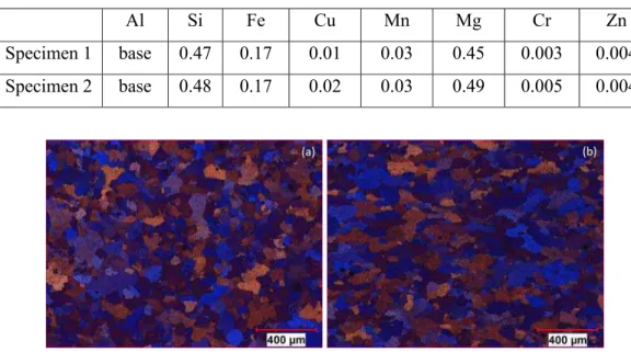
Three batches of AA 6063-O aluminium tubes, supplied by Alfiniti, were considered in the present investigation. Tubes outer diameter and wall thickness are 53.98 mm x 2.4 mm (batch A), 63.50 mm x 2.4 mm (batch B) and 69.85 mm x 2.4 mm (batch C). Two specimens were cut from two tubes from batch B for the chemical composition assessment. The chemical composition in wt. % of theses tubes was examined by optical emission spectrometry (OES) and is given in Table 1. The typical microstructure, determined by optical microscopy (Olympus/BX51M apparatus), is shown in Fig. 1 for both transversal (TD) and longitudinal directions (LD). Grains are equiaxed in both TD and LD directions. The average grain sizes measured from

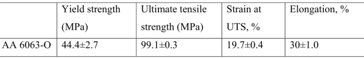
optical microscopy images are about 87µm and 88µm for the TD and LD directions respectively. Uniaxial tensile tests were carried out at room temperature using a hydraulic testing machine (MTS/ Alliance RT100). Six standard specimens were cut out from the tubes with 2.4 mm thickness and 12.5 mm wide gauge section. The gauge length of the specimen is 57 mm. The specimens were stretched up to fracture point under displacement control at constant speed of 3 mm/min. Based on the load-deformation curves, engineering stress-strain curve for this material were obtained and presented in Fig.2. Other mechanical properties of AA 6063-O tubes obtained from uniaxial tension tests are presented in Table 2.

Table 1. Chemical composition of AA 6063-O alloy (wt%)

Al Si Fe Cu Mn Mg Cr Zn

Specimen 1 base 0.47 0.17 0.01 0.03 0.45 0.003 0.004 Specimen 2 base 0.48 0.17 0.02 0.03 0.49 0.005 0.004

Figure 1. Typical microstructure of AA 6063-O for (a) transversal and (b) longitudinal directions (50X magnification)

Table 2. Mechanical properties of AA 6063-O tube Yield strength (MPa) Ultimate tensile strength (MPa) Strain at UTS, % Elongation, % AA 6063-O 44.4±2.7 99.1±0.3 19.7±0.4 30±1.0

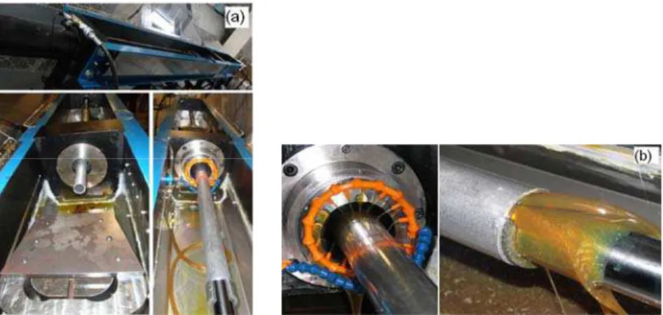
Drawing process was realized using a small hydraulic tube drawing machine illustrated in Fig. 3a. Tube pulling and mandrel pushing cylinders can implement maximum forces of 335 kN and 135 kN with strokes of 2.1m and 1.5m respectively. The swaged end of tube was clamped into a self locking tube gripper attached at the end of tube pulling cylinder. Optical and magnetic encoders were used to detect position of each axis while electronic pressure gages installed on both sides of each hydraulic cylinder to monitor the pressure. Fig. 4a and 4b show the images of the die and the mandrel respectively. Fig. 4c shows the die and mandrel installed in the drawing machine. The conical semi-angle of die and mandrel are α=10° and β=5.016° respectively. The distance between the die and mandrel is the dominant factor for determining thickness of tube with respect to the position of mandrel. But there are some other factors like springback of tube after drawing which will have effect on the thickness of tube. Therefore it is necessary to have an initial drawing to get an estimation of how much is the difference between the nominal thickness (distance between die and mandrel) and real thickness (thickness after drawing) then in the calibration step this value will be considered to compensate them by the mandrel motion. This calibration step provides the axial position of the mandrel as a function of times for obtaining required tube wall thickness. The mandrel position was continuously changed to reduce progressively the tube wall thickness up to the tube failure. During the tests, drawing lubrication was injected inside the tube (mandrel) by filling the tube with oil, and outside the tube (die), using multi-jets around the tube and in front of the die as shown in Fig. 3b. The lubricant utilized for all the tests was Magnus CAL 70-2 drawing oil. The machine operated at a low drawing speed of 6 mm/s. The thickness variation depends on the relative speed of mandrel and tube.

Figure 3. (a) Tube drawing machine (b) lubrication method

Figure 4. Tools utilized for variable thickness tube drawing: (a) die, (b) conical mandrel, (c) installed die and mandrel in the drawing machine.

After tube drawing, the tube minimum thickness and diameter at regions very close to fracture line but out of the necked zone were measured. The radial (_r) and circumferential (_c) strains were calculated by _r ln(h_f /h₀) and

0

ln( / )

c ODf OD

  , where OD0 and ODf are respectively the initial and final outer

diameters of tube and h0 and hf are the thicknesses of tube at the entrance and at the

exit of the die. The axial strain _acan be calculated based on the incompressibility condition: _a    . Therefore the limit values of the axial and circumferential  _{r c} strains were determined. These strains present the global or macroscopic strains. Additionally, for the tubes used for the formability limit experiments, square grids with an initial size of 3mmx3mm were electrochemically etched on the tube surface before the experiments. More details on the square grid analysis are available in the appendix A. Local axial and circumferential strains were measured using the square grid analysis technique in the region very close to fractured zone of the drawn tubes but out of necked zone. The average local strains values were compared with the macroscopic results presented previously.

The samples cut from the tube at the minimum thickness, have been analyzed using an Olympus BX51M upright microscope coupled to Clemex image-analysis software. Before optical microscope analysis, samples were mechanically polished using an automatic Tegrasystem grinding/polishing machine (sequentially 220 grits - 9µm - 3µm - 0.04µm) then electropolished using a fluoboric acid electropolishing solution from Fisher Scientific at 30 volts for 120 seconds.

3. Experimental results 3.1. Drawing processes

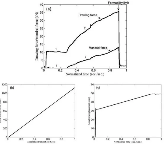
Fig. 5a shows the drawing and reaction forces on the mandrel from experimental results of the tubes which belong to the batch A. The tube drawing process with variable wall thickness has generally two principal steps: tube sinking step (denoted as 1 in Fig. 5a) and wall thickness reduction step (denoted as 2 in Fig. 5a). Figs. 5b and 5c show the tube and mandrel displacements used in the tube drawing for tubes from the batch A. It is well known that during the conventional tube drawing process, the drawing force increases quickly and reaches a steady state level, as mentioned by Neves et al. (2005). However, in variable wall thickness tube drawing process, the drawing force monitored during drawing is almost constant during tube sinking and increases as the mandrel comes into contact to reduce the wall thickness. The forces of tube sinking are about 10 kN, 22.5 kN and 31.5 kN for the batches A, B and C respectively. During the drawing process, the drawing and the mandrel force increase until the maximum values are obtained. This state is called the limit state or in another words, the tube formability limit (Fig. 5a). The maximum force of all tubes drawing is about 35.21 kN, 40.73 kN and 43.74 kN for the A, B and C batches respectively. The maximum force exerted on the mandrel is about 13.16 kN, 9.79 kN and 5.18 kN for the A, B and C batches respectively. The outside and inside surface finishes of the tube using the tapered mandrel are good (inside and outside surface finishes are in the range of 0.17-0.3µm and 0.52-0.62µm respectively). The surface finish of initial tubes is about 0.74µm and 0.75µm for the inside and outside surfaces respectively. It can be seen that using a tapered mandrel, better surface finish is achieved. Fig. 6 shows the fracture of the head of the tube with variable wall thickness.

Figure 5. Experimental results: (a) drawing force and reaction force on the mandrel, (b) tube displacement and (c) mandrel displacement

Figure 6. Fracture of the tube head with variable wall thickness

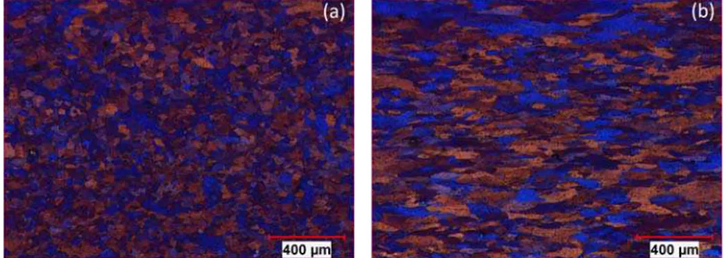
3.2. Microstructure at the limit state

In order to characterize the microstructure of tube at the limit state, several cut samples from the tubes were observed using the optical microscope. The observations in the both transversal and circumferential directions of tube were realized for establishing the anisotropy of drawn tubes.

microstructure at the limit state of tube for the tubes from batch A. As it was expected, grain elongation along the axial direction (LD observations) of drawn tube was observed (Fig. 7b). The refinement of grains was observed in both TD and LD directions too. The refinement of grains is observed on the material deformed at large strain or at the dynamic plastic deformation regime, as reported by Bui et al. (2008). Here, the grain refinement is also observed at the limit state of variable wall thickness tube drawing because the materials deformed at very large triaxial deformation which induces anisotropy in the microstructure and mechanical properties of drawn tube.

Figure 7. Morphology of grains in the drawn tube belonged to the batch A at the limit state: (a) TD direction and (b) LD direction

3.3. Strain field at the limit state

The critical values of axial and circumferential strains measured by the grid analysis method are given in Table 3. These measured values are comparable with the values calculated by the measurement of tube dimensions. As it was expected, high triaxial strains caused refinement of grains in the drawn tubes as confirmed in the previous section.

Table 3. Strains at the limit state

a

 _r _c

Batch A Square grid 0.519 -0.367 -0.152 Final dimension 0.507 -0.377 -0.130 Batch B Square grid 0.540 -0.224 -0.316 Final dimension 0.517 -0.223 -0.294 Batch C Square grid 0.570 -0.143 -0.427 Final dimension 0.548 -0.158 -0.390

3.4. Formability limit of aluminium tube drawing with variable wall thickness

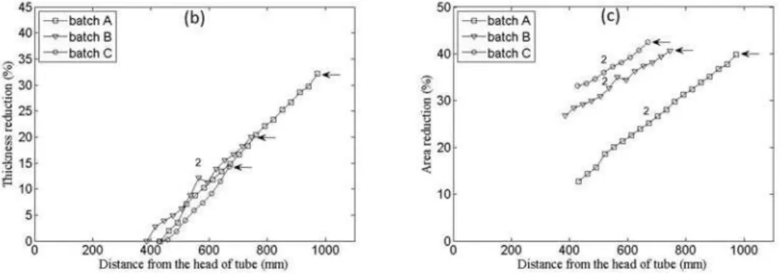
The drawn tubes were cut into two parts to achieve better measurement of thickness distribution in the axial direction of tube. The results presented in Fig.8a show the variation of the wall thickness measured on the tube after drawing processes in axial direction of tube. The minimum thickness achieved immediately before tube breakage are 1.65mm, 1.93mm and 2.05mm for the A, B and C batches respectively. Fig. 8b shows the corresponding wall thickness reduction. The limit values are 32.17%, 20.02% and 14.2% for the A, B and C batches respectively. In Fig. 8c the corresponding area reductions were presented. The limit values are 39.83%, 40.58% and 42.48% for the A, B and C batches respectively. The limit thickness and limit area reduction were calculated and reported in Table 4. The maximum drawing stress is obtained by dividing the maximum axial drawing force over minimum tube area. The average of maximum drawing stress is about 150 MPa. The drawing stress ratio over initial yield stress i.e. _z Yis about 3.4 for all tubes whatever the outer diameter. This value can be considered as a forming criterion for AA 6063-O tube. This criterion is independent of tube outer diameter. It is function of mechanical properties of material as suggested by Rubio et al. (2006), of geometry and type of die and mandrel as suggested by Yoshida et al. (2004), and process parameters (i.e. friction coefficients and temperature conditions) as suggested as Semiatin and Jonas (1984). In the next section, an extension of an analytical model is proposed for determination of drawing stress. By using the critical value 3.4, the formability or in other words minimum achievable tubes thickness can be predicted.

Figure 8. (a) Variation of the wall thickness measured on the tubes after drawing process, (b) Corresponding wall thickness reduction and (c) corresponding area reduction. The arrows show the limit states. Sinking step denoted as 1, wall thickness

13 Table 4. Summary of the experimental results for AA 6063-O tubes

Initial outer diameter (mm) Initial thickness (mm) Fmand-max (kN) Fdraw-max (kN) Final outer diameter (mm) Minimum thickness (mm) Maximum area reduction (%) Maximum thickness reduction limit (%) σdraw (MPa) σdraw/Y Batch A 53.98 2.4 13.16 35.21 47.3 1.65 39.83 32.17 150.49 3.39 Batch B 63.49 2.4 9.79 40.73 47.3 1.93 40.58 20.02 148.14 3.34 Batch C 69.85 2.4 5.18 43.74 47.3 2.05 42.48 14.2 151.40 3.41

4. Analytical methods for studying the aluminium tube drawing formability limit

While techniques of tube sinking, tube drawing with a mandrel and tube drawing with floating plugs are well known processes, the modification of a conical mandrel proposed in this paper for producing variable thickness aluminium tubes is quite new; therefore numerical and/or analytical methods are necessary to control and optimize the process.

Many analytical and numerical studies about different shapes of drawn tubes have been published since fifty years ago. Various aspects of tube drawing processes have been analytically evaluated using energy, slab, and upper bound methods. Rubio et al. (2006) applied upper bound method to analyze the energy of thin-walled tube drawing processes in conical converging dies with inner plugs, based on the assumption that the process occurs under plane strain and Coulomb friction conditions. Rubio (2006) compared the results obtained by both slab and upper bound methods based on the same assumption in the former cited paper. Wang et al. (2008) proposed a new mathematical model by modifying the conventional slab model developed by Rubio (2006) and mentioned that the modified slab method is useful to predict the behaviour of the high-reduction-ratio drawing process with a floating plug. Um et al. (1997) proposed an upper-bound solution for axisymmetric tube drawing through a conical die with a fixed tapered plug. In the present investigations, the same type of die and mandrel was used. Therefore, the analytical model based on the upper bound methods, obtained by Um et al. (1997), is applied.

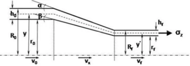
Figure 9. The schematic view of the tubes drawing process

In metal-forming processes such as rolling, extrusion, tube drawing etc., the plastic strain is very large compared to the elastic strain. Therefore, the material behavior can be described like the fluid flow as mentioned in Venkata Reddy et al. (1996). Under these conditions the strain rate can be defined in terms of velocity. In this paper, the

tube material is assumed to be isotropic, incompressible and follows a plastic behavior. The Lévy-Mises equation was used as the constitutive law for relating the stresses and strains of tube material (see appendix B for more detail).

A schematic view of axisymmetric tubes drawing process with conical die and mandrel is shown in Fig. 9. The process variables related to the geometry are: (i) the die semiangle, α; (ii) the mandrel semiangle, β; (iii) and the tube cross-sectional area reduction, r: 0 0 f A A r A   (1)

where A0 and Af are the initial and final areas of the tube, respectively and can be

calculated as follows:

  



  



where R0 and Rf represent the initial and final outer radii of tube, respectively and h0

and hf are the thicknesses at the entrance and at the exit of the die respectively.

In accordance with the upper-bound theorem (Avitzur 1979), the total energy consumption _{I should be minimized for the actual velocity distribution. The total} *

energy consumption in the case of tube drawing is:

*

H f f r

I W W W W (4)

where W_H, W , _f W , _f W_r are the rate of energy dissipations due to homogeneous deformation, at the outer interface, at the inner interface and due to internal shear, respectively. These energy dissipation rates were obtained from analytical solutions proposed in Um et al. (1997) and presented with more detail in the appendix B:

2 1 2 0 0 0 0 0 2 (1 ) ln 3 H f A Y W y y A v A     ₍₅₎

0 0 0 0 0 0 2 1 1 ln ln sin 2 1 1 f f f f i f f f f f R R t R t r R R t R t r A v W t R r t R r               _{ }  _{ }       ₍₆₎ 0 0 0 0 0 0 2 1 1 ln ln sin 2 1 ( ) 1 ( ) f f f f i f f f f f R R t R t r R R t R t r A v W t R r t t R r t      _         _  _          ₍₇₎ 2 2 2 2 0 0 0 0 0 0 0 0 0 2 tan 3 3 ( ) ( ) f f f f r f f f R R r r R R r r Y W A v R R r R R r        _  _        ₍₈₎

where ttan tan; Y the yield strength; r0 and rf are inner radii of the initial and

final tube, respectively; v₀the incoming velocity of the tube; v_foutgoing velocity of

the tube; _iand _i are shear stresses at the interface between the die - tube and between the tube – mandrel, respectively.

Two shear stresses, , between two sliding interfaces can be defined using two different assumptions. If Coulomb type assumption is used, the shear stress is proportional to the pressure, p, between the surfaces in contact according to the expression  p, where the proportional coefficient,, is called Coulomb friction coefficient. If the partial friction hypothesis is used, the shear stress,  , is assumed to be proportional to the shear yield stress, k, and given by  mk, where m is the partial friction coefficient (0≤m≤1). The partial friction coefficient m, was referred as the frictional shear factor, can take the value m=0 for a frictionless interface and m=1 for sticking friction, as mentioned in Schey (1983). Altan et al. (1983) mentioned that in cold forming of aluminum alloys, the values of m vary from 0.05 to 0.15 using conventional phosphate-soap lubricants or oils.

In this paper, we used the partial friction hypothesis between the die-tube and between tube-mandrel interfaces with values mand m respectively. These shear stresses may be expressed as:

i m k     (9) i m k     (10)

where 3 Y

k is shear yield stress of tube material.

More details on this model are available in Um et al. (1997).

The upper-bound on the drawing stress is then determined as (Um et al. (1997)):

* 0 0

zA vf f zA v I

   (11)

Finally, we can define the drawing stress from Eqs. (4-8) and (11) as follow

2 2 2 2 2 1 2 0 0 0 0 0 0 0 0 0 0 0 0 0 0 0 0 0 2 2 (1 ) ln tan 3 ( ) ( ) 3 3 2 1 1 ln ln sin 2 1 1 2 1 1 ln ln sin 2 1 ( ) 1 f f f f z f f f f f f f f i f f f f f f i f f R R r r A R R r r Y Y y y A R R r R R r R R t R t r R R t R t r t R r t R r R R t R t r R R t R r t t                    _  _                _{ }  _{ }                0 ( ) f f f f t R t r R r t      _      (12)

The solutions given in the conventional model were generally applied to a static geometry (without motion of mandrel). During the variable wall thickness tube drawing process, the position of mandrel is moving (as shown in the Fig. 5c). The related geometries (i.e. inner radius, wall thickness of tube at the exit of die) were subject to change during the process. The next section presents this model adapted to the case of variable thickness tube drawing process.

5. Application of the model and discussions

This section reveals the abilities of the extended model to determine the drawing stress and the formability limit of variable thickness tube drawing.

5.1. Application of upper bound method to determine drawing stress in the variable thickness tube drawing process

During tube drawing process, the conical mandrel moves inside the die. The thickness at the exit of the die is reduced and the cross sectional area reduction increases

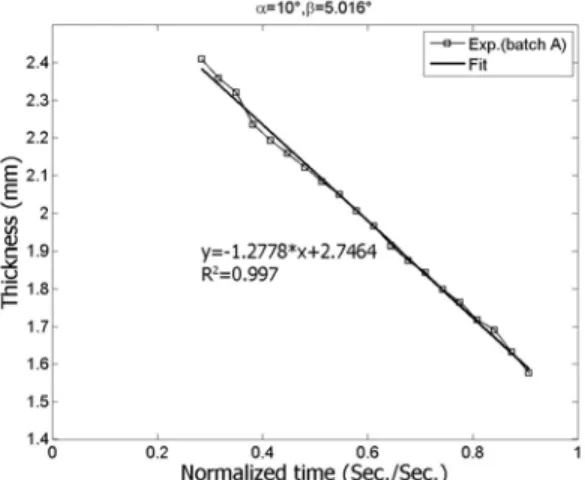
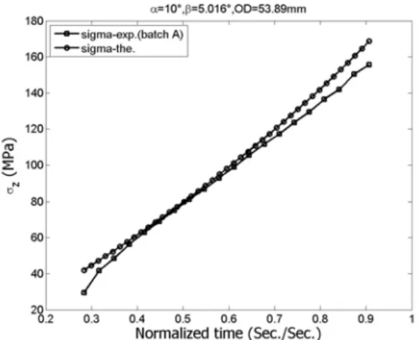
progressively. For the model application, a linear variation of wall thickness is applied for the simulation of tube drawing, but there is no limitation on the rate of change of the wall thickness. The analytical model of the variation of wall thickness can be obtained by fitting the experimental tube wall thickness versus time curve (Fig. 10). A linear function y=-1.2778*x+2.7464 was found. This linear function of tube wall thickness corresponds to the tube and mandrel displacements shown in Figs. 5b and c. Fig. 11 shows the drawing stress evolution versus normalized time. A normalized time is defined as the ratio of present time to the total time of tube drawing process. In the first step of computation, we tried to identify the friction coefficients at mandrel-tube and die-mandrel-tube interfaces by calibrating the results of the analytical model and measurement by iterative process. The calibrated friction coefficients are determined when the drawing stress from upper bound method and from the experimental tests are approximately the same (Fig. 11). The obtained partial friction coefficients are m=0.13, m=0.13 for the die-tube and tube-mandrel interfaces, respectively. In the finite element model presented by the Bihamta et al. (2010a and b) they used Coulomb friction coefficient in their studies, but here our formulations were based on the partial friction coefficient (m). The used friction coefficients in this study is in good correspondence with the suggested values for the m for the aluminum alloys cold forming in Altan et al. (1983).

Figure 10. Variation of tube wall thickness (batch A) versus normalized time during single pass drawing process

Figure 11. Evolution of tube drawing stress versus normalized time (batch A)

Fig. 12 shows the drawing stress evolution versus normalized time for different outer diameters. It is clear that the drawing stress in the tubes at the exit of the die increases during the process. The predicted values for the tubes with larger outer diameters are higher than the smaller ones for the same normalized time.

Figure 12. Evolution of drawing stress versus normalized time for the tubes with various outer diameters.

5.2. Application of upper bound method to determine the formability limit of variable thickness tube drawing process

The formability limit of tube drawing is determined when the drawing stress ratio is equal to 3.4. This limit has been plotted on the Fig 13. The wall thickness and the area reduction limits can be determined using the intersection between horizontal line and the drawing stress ratio curve for different tube dimensions (batches A, B and C) as

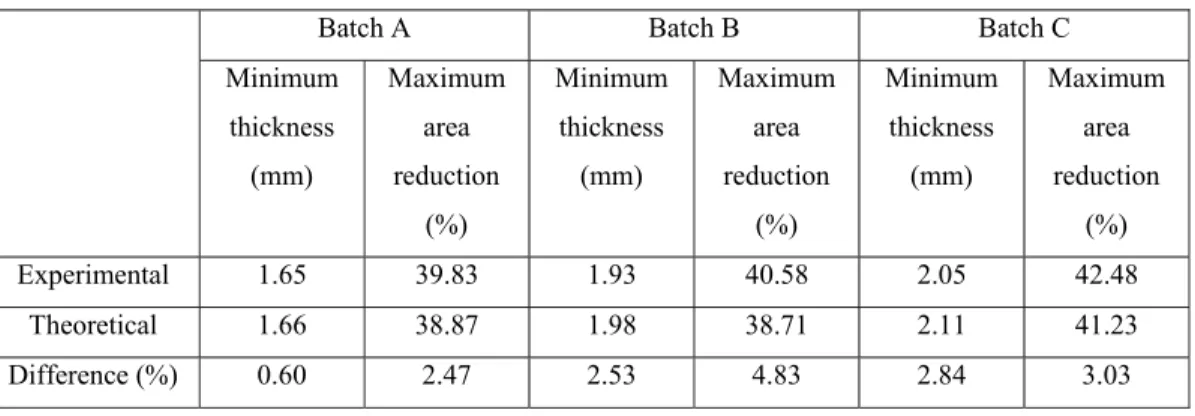
shown in Fig. 13a and 13b. Fig. 14 shows the comparison between predicted and experimental values. The values are presented with more details in Table 5. There is a very good agreement between the theoretical and experimental results; the maximum differences are 2.8% and 4.8% for minimum thickness and maximum area reduction respectively.

Figure 13. (a) Evolution of drawing stress ratio versus wall thickness and (b) area reduction for tubes of initial fixed thickness h0=2.4mm and of various outer diameters

Figure 14. Comparison of analytical (the.) and experimental (exp.) values of formability limit: (a) area reduction limit (b) thickness limit

Table 5. Comparison between predicted and experimental values of formability limit

Batch A Batch B Batch C

Minimum thickness (mm) Maximum area reduction (%) Minimum thickness (mm) Maximum area reduction (%) Minimum thickness (mm) Maximum area reduction (%) Experimental 1.65 39.83 1.93 40.58 2.05 42.48 Theoretical 1.66 38.87 1.98 38.71 2.11 41.23 Difference (%) 0.60 2.47 2.53 4.83 2.84 3.03

Fig. 14b shows that for a fixed initial tube thickness, the smaller diameter tubes can be drawn with smaller thickness limit than larger ones. However, when the formability limits of tubes with different initial thickness were compared, it is not sure that the smaller diameter can be drawn much more than the larger ones. Thus, the proposed model can be applied to predict the effect of both initial tube outer diameter and thickness on the formability limit.

Figs. 15a and 15b show the evolution of drawing stress ratio versus wall thickness and area reduction for the tubes of initial fixed outer diameter OD=53.98mm and of initial thickness varying in the range of 2.4 to 3.0mm. The horizontal lines present the position of formability limit (i.e. _z/Y=3.4) and the intersection between horizontal lines and the drawing stress ratio curve gives the thickness and area reduction limits. The Fig. 16 shows the evolution of formability limit as function of initial tube wall thickness for the tube of OD=53.98mm. It was found that for a fixed tube outer diameter, the tubes with smaller thickness have the smaller area reduction and thickness limits reduction.

Figure 15. (a) Evolution of drawing stress ratio versus wall thickness and (b) area reduction for OD=53.98mm and various initial tube thicknesses

Figure 16. Evolution of formability limit: (a) area reduction limit (b) thickness limit as function of initial tube thickness for the tube of OD=53.98mm

Tables 6 and 7 predict the variation of area reduction and thickness limits of tubes as a function of initial tube thickness and outer diameter. It was suggested from the Table 7 that for the tubes with initial wall thickness from 2.4mm to 3.0mm and outer diameter from 53.98 to 69.85mm, the minimum thickness of drawn tubes can change from 1.66mm to 2.23mm. This datasheet may be useful in the choice of initial tube dimension to produce the variable wall thickness tube with the required dimensions. Table 6. Area reduction limit (%) for tubes of different wall thicknesses and outer diameters 0 h (mm) 2.4 2.5 2.6 2.7 2.8 2.9 3.0 OD (mm) 53.98 38.87 40.50 41.33 42.74 44.05 44.66 45.81 56.00 37.78 39.49 40.41 41.89 43.26 44.53 45.16 58.00 37.33 39.09 40.70 41.60 43.01 44.32 45.54 60.00 37.57 39.34 40.98 41.91 43.34 44.66 45.89 63.50 38.71 40.49 42.13 43.10 44.52 45.84 47.07 66.00 39.38 41.16 42.80 44.31 45.72 47.02 48.24 69.85 41.23 42.95 44.56 46.04 47.42 48.71 49.91

Table 7. Thickness limit (mm) for tubes of different wall thicknesses and outer diameters 0 h (mm) 2.4 2.5 2.6 2.7 2.8 2.9 3.0 OD (mm) 53.98 1.66 1.68 1.72 1.74 1.76 1.80 1.82 56.00 1.76 1.78 1.82 1.84 1.86 1.88 1.92 58.00 1.84 1.86 1.88 1.92 1.94 1.96 1.98 60.00 1.90 1.92 1.94 1.98 2.00 2.02 2.04 63.50 1.98 2.00 2.02 2.07 2.09 2.11 2.13 66.00 2.04 2.07 2.09 2.11 2.13 2.15 2.17 69.85 2.11 2.13 2.15 2.17 2.19 2.21 2.23

Whole formability limit of tubes presented in this paper is for the case of fixed die (with semi-angle  10o

) and mandrel (with semi-angle  5.016o

). The formability limit of initial tube geometry can be determined analytically as shown in Tables 6 and 7. However, the experimental studies realized by Yoshida et al. (2004) suggested that the formability limit depends strongly on the geometry of die and mandrel. It was also suggested that the thickness limit presented in the Table 7 can be reached the smaller values when the optimal die and mandrel geometries were used. The optimization of die and mandrel geometries is not the objective of this study. However, this paper suggested that the minimization of drawing stress ratio for

increasing the formability of tube during process may be used as one of the optimization objectives.

As mentioned in the introduction section, several previous researches were developed to study the formability limit of constant wall thickness tubes. Tong et al. (2009) and Tong et al. (2009) used the ductile fracture criterion of the discrete Cockcroft-Latham equation combined with the finite element analysis to establish the drawing limit graphs of magnesium and aluminium tubes, respectively. These graphs give the possible initial tube thickness and tube diameter for a definite final tube without failure. For the first time, the present study investigates the formability limit and provides the influence of initial tubes geometry on the formability limit in the case of variable wall thickness tube drawing process.

6. Conclusion

A new experimental methodology to investigate the formability limit of single pass tube drawing process was proposed. Tube drawing tests were performed on aluminium tubes for determining the formability limit. A development of upper bound solution, combined with a maximum drawing stress ratio forming criterion, was proposed. The following results were obtained:

- The moving conical mandrel can be used in the tube drawing process to produce tubes with variable wall thickness and the minimum wall thickness will be obtained when the tube reaches to its formability limit.

- A microstructure change (i.e. grain refinement and elongation) is observed at the limit state of tube.

- The wall thickness limits of AA 6063-O tubes in a single drawing pass are different for various initial outer diameters. However, their area reduction limits were always about 40%.

- The analytical model based on the upper bound method predicts the drawing stress in tube drawing process correctly.

- The experimental studies of tube drawing with various outer diameters confirmed the results of theoretical consideration and the proposed formability criterion can be used to determine the tube formability.

Finally, the forming criterion proposed in this study can be used to optimize die and mandrel geometries. With that criterion, new aluminium tubes will be drawn with

high thickness reductions. These tube will be hydroformed for automotive and bicycle applications.

Acknowledgements

The authors thank the National Sciences and Engineering Research Council of Canada, Alfiniti, Aluminerie Alouette, C.R.O.I and Cycles Devinci for the financial support of this research. A part of the research presented in this paper was financed by the Fonds Québécois de la Recherche sur la Nature et les Technologies (FQRNT) by the intermediary of the Aluminium Research Centre – REGAL. The authors want to express special thanks to their colleagues at Aluminium Technology Centre (ATC) (Genevieve Simard, Myriam Poliquin, Martin Pruneau, Michel Perron and Jean François Béland) for their technical supports in experiments.

Appendix A

Local strains can be measured using the square grid analysis technique. The grid patterns, consisted of electrochemically-marked orthogonal lines spaced 3 mm, were made on the tube surface. When the tube deforms during drawing process the grid patterns deform too (see Fig. 17).

Figure 17. (a) Illustration of the deformation of grid patterns on the tube surface. (b) Grid pattern before (on initial tube) and after (on drawn tube) deformation. The local

axial and circumferential strains were measured at the limit state (between two parallel solid lines)

The local axial and circumferential strains can be generally determined as: 2 0 2 0 ln L z L L dz z L  





In the present work, the local axial and circumferential strains were measured via Autogrid, an automated strain measurement system equipped with four cameras. Only the strain values at the limit state were considered to calculate the average local strains values (Fig. 17b).

Appendix B

The rate of energy dissipations due to homogeneous deformation, at the outer interface, at the inner interface and due to internal shear can be calculated as (Um et al. 1997):

B.1. Energy dissipations due to homogeneous deformation

The plastic deformation work increment per unit volume dw is calculated by:

11 11 22 22 33 33 2( 12 12 23 23 31 31)

dw             (B.1)

There is no shear strain in the homogeneous deformation. Therefore, the homogeneous deformation work per unit volume, dw , is _H

11 11 22 22 33 33

H

dw       (B.2)

In the case of tube drawing, Eq.(B.2) can be expressed as:

H a a r r c c

dw       (B.3)

where _a, _rand _c are the axial, radial and circumferential stresses, respectively. and _a,_rand _care the axial, radial and circumferential strains, respectively. The Lévy-Mises equations can be expressed as:

2 3 2 r c a a d  d _   _   (B.4) 0 2 (1 ) 3 2 a c r r a d  d _   _  y d   (B.5) 0 2 3 2 r a c c a d  d _   _ y d   (B.6)

The circumferential, radial and axial strains can be expressed as:

0 0 ln f f c R r R r     (B.7) 0 0 ln f f r R r R r     (B.8) and 2 2 0 0 2 2 ln a c r f f R r R r         (B.9) It follows that: 2 2 0 0 0 2 2 0 0 ln f f ln c f f a R r d R r y R r R r d         (B.10)

The Eq. (B.3) becomes:

2 2 2 2 0 1 2 ( ) ( ) ( ) 3 3 H a r r c c a dw  d _        _ d (B.11)

where ₀is the uniaxial yield stress. The homogeneous strain can be expressed as:

1 2 2 2 2 2 ( ) ( ) ( ) 3 H a r r c c a d  _ d d  d d  d d _ (B.12)

Substituting Eq. (B.4-6) in to Eq. (B.12):

1 2 ₂ 0 0 0 2 2 (1 ) 3 3 H a d  y y d  d (B.13)

And it follows from Eqs. (B.11) and (B.13) that: 1 2 0 2 0 0 0 2 (1 ) 3 H H a dw d    y y d (B.14) Therefore: 1 1 2 2 0 2 0 2 0 0 0 0 0 2 2 (1 ) (1 ) ln 3 3 H a f A w y y y y A  _          _ _   (B.15)

The rate of energy dissipation due to homogeneous deformation is given by:

1 2 0 2 0 0 0 0 0 2 (1 ) ln 3 H f A W y y A A  _      _ _    _(B.16)

B.2. Energy dissipations due to internal shear

At the entry, the rate of energy dissipation over a differential ring area, dA, at any arbitrary y is: * 0 2 ( ) 0 2 2 tan A A y dW y dy k k y dy R         _(B.17)

where k is the shear yield stress of tube material.

The rate of energy dissipation over the entire area at the entry is:

0 0 3 3 2 0 0 0 0 0 0 2 2 tan tan 3 R A r R r W k y dy k R R        

_

where A₀ (R₀2r₀2)is the initial cross sectional area of the tube.

At the exit, the rate of energy dissipation over a differential ring area at any arbitrary y’ is: ’ ’ ’ * ’2 ’ ( ) 2 2 f tan B _{B y} f dW y dy k k y dy R         _(B.19)

where _f is the horizontal velocity of a particle at the exit. Therefore, the rate of energy dissipation over the entire area at the exit is:

3 3 ’2 ’ 2 2 tan tan 3 f f R f f f B f f r f R r W k y dy k R R        



It follows from Eqs. (B.19) and (B.20) that the total rate of energy dissipated along these two discontinuities is:

2 2 2 2 0 0 0 0 0 0 0 0 0 0 2 tan ( ) ( ) 3 3 f f f f r f f f R R r r R R r r W A R R r R R r  _{ }       _  _        _(B.21)

B.3. Energy dissipations due to outer interface at the inner interface

A ring slab whose outer and inner radii are R and r at some arbitrary position in the deformation zone is considered. The outer and inner contact areas of the slab are

sin

dr anddr sin , respectively. The rate of energy dissipation dW at the outer _f interface is: ( ) 2 sin f i S C dR dW R      _(B.22)

where _iand _{S C( )}are the shear stress and velocity of a particle at the outer interface at position x, respectively. The velocity is related to the horizontal velocity_x:

( ) cos

S C x

   (B.23)

Constancy of volume requires:









0 0 0

x R r R r

    (B.24)

It follows from Eqs. (B.23) and (B.24) that:









Therefore, the rate of energy dissipation at the outer interface is given by:











It follows from the geometry that:





The combination of Eqs. (B.26) and (B.27) gives:











Similarly, the rate of energy dissipation at the inner interface is given by:

0 0 0 0 0 0 2 1 1 ln ln sin 2 1 ( ) 1 ( ) f f f f i f f f f f R R t R t r R R t R t r A v W t R r t t R r t                _{ }  _{ }       _(B.30)

References

Alexandrova, N., 2001. Analytical treatment of tube drawing with a mandrel. Journal of Mechanical Engineering Science, 215, pp. 581–589.

Alexandrova, N., 2003. Fracture analysis of tube drawing with a mandrel. Journal of Materials Processing Technology, 142, Issue 3, pp. 755-761.

Alexoff, R.L., 2004. Method and apparatus for producing variable wall thickness tubes and hollow shafts, U.S. Patent no. 6807837, Oct.26.

Altan, T., Oh, S.L., Gegel, H. L., 1983. Metal Forming: Fundamentals and Applications. American Society for Metals, Metals Park, Ohio.

Avitzur, B., 1979. Metal Forming: Processes and Analysis, R. E. Krieger Publishing Co., New York.

Banabic, D., Bunge, H.J., Pohlandt, K., Tekkaya, A.E., 2000. Formability of metallic materials, Springer Verlag, Berlin.

Bihamta, R., D’Amours, G., Rahem, A., Guillot, M., Fafard, M., 2010a. Numerical studies on the production of variable thickness aluminium tubes for transportation purposes, SAE World Congress, Detroit, April.

Bihamta, R., D’Amours, G., Bui, Q. H., Rahem, A., Guillot, M., Fafard, M., 2010b. Optimization on the production of variable thickness aluminum tubes. Proceedings of the ASME 2010 International Manufacturing Science and Engineering Conference MSEC2010, October 12-15, 2010, Erie, Pennsylvania, USA.

Bui, Q.H., Dirras, G. F., Hocini, A., Ramtani, S., Abdul-latif, A., Gubicza, J., Chauveau, T., Fogarassy, Z., 2008. Microstructure and mechanical properties of commercial purity HIPed and Crushed Aluminum. Materials Science Forum, 584-586, pp. 579-584.

Guillot, M., Fafard, M., Girard, S., Rahem, A., D’Amour, G., 2010. Experimental study of the aluminum tube drawing process with variable wall thickness, SAE World Congress, Detroit, April.

Hill, R., 1963. A general method of analysis for metal-working processes. Journal of the Mechanics and Physics of Solids, 11, pp. 305–326.

Hwang, Y.M., Lin, Y.K., Chuang, H.C., 2009. Forming limit diagrams of tubular materials by bulge tests. Journal of Materials Processing Technology, 209, Issue 11, pp. 5024-5034.

Kim, S.W., Kwon, Y.N., Lee, Y.S., Lee, J.H., 2007. Design of mandrel in tube drawing process for automotive steering input shaft. Journal of Materials Processing Technology 187-188, pp.182-186.

Komori, K., 2003. Effect of ductile fracture criteria on chevron crack formation and evolution in drawing. International Journal of Mechanical Sciences, 45, Issue 1, pp. 141-160

Neves, F.O., Button, S.T., Caminaga, C., Gentile, F.C., 2005. Numerical and experimental analysis of tube drawing with fixed plug. Journal of the Brazilian Society of Mechanical Sciences and Engineering, 27, pp. 426-431.

Oh, S.I., Chen, C.C., Kobayashi, S., 1979. Ductile Fracture in axisymmetric extrusion and drawing. Part 2, Workability in extrusion and drawing. Journal of Engineering for Industry, 101, pp. 37-44.

Rubio, E. M., 2006. Analytical Methods Application to the Study of Tube Drawing Process with Fixed Conical InnerPlug: Slab and Upper Bound Methods. Journal of Achievements in Materials and Manufacturing Engineering, 14, pp. 119−130.

Rubio, E.M., González, C., Marcos, M., Sebastián, M.A., 2006. Energetic analysis of tube drawing processes with fixed plug by upper bound method. Journal of Materials

Processing Technology, 1–3 (177), pp. 175–178.

Tong Y., Quan G., Chen B., 2009. Constitutive description for drawing limit of magnesium alloy tube based on continuum damage mechanics. Materials Science Forum, 610-613, pp. 951-954

Tong Y., Quan G., Chen B., 2010. A study on Al-6061-T6 tube drawing limit based on critical damage value. Materials Science Forum, 102-104, pp. 69-73

Schey, J.A., 1983. Tribology in metalworking: friction, lubrication, and wear. American Society for Metals, Metal Park, Ohio.

Schmid, W., Reissner, J., 1982. Critical deformation in the ironing of deep-drawn cups. Journal of Materials Processing Technology, 24, pp. 597-604.

Semiatin, S.L., Jonas, J.J., 1984. Formability and Workability of Metals: Plastic Instability and Flow Localization, ASM Series in Metal Processing.

Um, K.K., Lee, D.N., 1997. An upper bound solution of tube drawing. Journal of Materials Processing Technology, 63, Issues 1-3, pp. 43-48.

Venkata Reddy, N., Sethuraman, R., Lal, G.K., 1996. Upper-bound and finite-element analysis of axisymmetric hot extrusion. Journal of Materials Processing Technology, 57, pp. 14-22.

Vujovic, V., Shabaik, A. H., 1986. A New Workability Criterion for Ductile Metals. Journal of Engineering Materials and Technology, 108, pp. 245-249.

Wang, C.S., Wang, Y.C., 2008. The theoretical and experimental of tube drawing with floating plug for micro heat-pipes. Journal of mechanics, 24, pp. 111-117.

Yoshida, K., Furuya, H., 2004. Mandrel drawing and plug drawing of shape-memory-alloy fine tubes used in catheters and stents. Journal of Materials Processing Technology, 153-154, pp. 145-150.