Publisher’s version / Version de l'éditeur:
Lighting Research and Technology, 37, June 2, pp. 93-115, 2005-06-01
READ THESE TERMS AND CONDITIONS CAREFULLY BEFORE USING THIS WEBSITE. https://nrc-publications.canada.ca/eng/copyright
Vous avez des questions? Nous pouvons vous aider. Pour communiquer directement avec un auteur, consultez la première page de la revue dans laquelle son article a été publié afin de trouver ses coordonnées. Si vous n’arrivez pas à les repérer, communiquez avec nous à PublicationsArchive-ArchivesPublications@nrc-cnrc.gc.ca.
Questions? Contact the NRC Publications Archive team at
PublicationsArchive-ArchivesPublications@nrc-cnrc.gc.ca. If you wish to email the authors directly, please see the first page of the publication for their contact information.
This publication could be one of several versions: author’s original, accepted manuscript or the publisher’s version. / La version de cette publication peut être l’une des suivantes : la version prépublication de l’auteur, la version acceptée du manuscrit ou la version de l’éditeur.
For the publisher’s version, please access the DOI link below./ Pour consulter la version de l’éditeur, utilisez le lien DOI ci-dessous.
https://doi.org/10.1191/1365782805li132oa
Access and use of this website and the material on it are subject to the Terms and Conditions set forth at Lighting quality research using rendered images of offices
Newsham, G. R.; Richardson, C.; Blanchet, C.; Veitch, J. A.
https://publications-cnrc.canada.ca/fra/droits
L’accès à ce site Web et l’utilisation de son contenu sont assujettis aux conditions présentées dans le site LISEZ CES CONDITIONS ATTENTIVEMENT AVANT D’UTILISER CE SITE WEB.
NRC Publications Record / Notice d'Archives des publications de CNRC: https://nrc-publications.canada.ca/eng/view/object/?id=b0e1797a-c736-4b19-b305-b207e2f99517 https://publications-cnrc.canada.ca/fra/voir/objet/?id=b0e1797a-c736-4b19-b305-b207e2f99517
Lighting quality research using rendered images of offices
Newsham, G.R.; Richardson, C.; Blanchet, C.; Veitch, J.A.
NRCC-47072
A version of this document is published in / Une version de ce document se trouve dans : Lighting Research & Technology, v. 37, no. 2, June 2005, pp. 93-115
Doi: 10.1191/1365782805li132oa
Lighting Quality Research using Rendered Images of Offices
Newsham, G.R., Ph.D.; Richardson, C.; Blanchet, C.; Veitch, J.A., Ph.D. Institute for Research in Construction
National Research Council Canada Montreal Rd., Ottawa, Ontario
K1A 0R6, Canada
Responsible Author: Guy Newsham Tel: (613) 993-9607; Fax: (613) 954-3733
e-mail: guy.newsham@nrc-cnrc.gc.ca
Abstract
Forty participants viewed a series of high-quality, colour images of a
typical open-plan partitioned office, and rated them for attractiveness. The images were projected at realistic luminances and 33% of full size. The images were geometrically identical, but the outputs of four lighting circuits depicted in the renderings were independently manipulated. Initially, the lighting circuit outputs were random, but a genetic algorithm was used to generate new images that retained features of prior, highly-rated, images. As a result, the images converged on an individual’s preferred scene. Luminances in the preferred image were similar to preferred luminances chosen by people in real settings. A sub-set of images was rated on Brightness, Non-Uniformity and Attraction scales. Ratings were
significantly related to simple photometric descriptors of the images. In particular, around 50% of the variance in Attraction ratings was predicted by average image luminance and its square, or by average image
1. INTRODUCTION
The traditional method of exploring preferred luminous conditions involves participants evaluating full-scale spaces lit in different ways. These
studies are expensive, especially if one wishes to manipulate the lighting design between evaluations. There has been some interest, from both researchers and lighting designers, in other presentation methods, such as scale models, photographs, or computer renderings. Research in areas such as forestry, architecture and urban design [e.g. Daniel & Meitner, 2000; Danford & Willems, 1975; Rohrmann & Bishop, 2002; Bishop & Rohrmann, 2003] have established that images can be a reasonable surrogate for the real space, particularly on ratings related to aethestics. The limited lighting research on this topic concurs with this, when using photographs [Hendrick et al., 1977], or highly-detailed simulations [Mahdavi & Eissa, 2002].
However, these studies were limited to the evaluation of predefined scenes. With this approach one can compare ratings of images to real spaces, find which of a set of images is most preferred, and look for general trends, but one cannot easily find the optimal scene. Johnston [1999] and Johnston & Franklin [1993] described an interesting method using computer-generated images of faces to arrive at an optimally attractive face. Software initially presented a series of faces with random variations of features (e.g., hair colour, size of chin, separation of eyes). A participant rated each face for attractiveness. Using a genetic algorithm, the software then combined the most attractive faces to produce new combinations of faces and the rating process was repeated until a face with an optimal rating was arrived at. This proved to be an effective method of finding an optimally attractive face from a vast combination of possible faces. Furthermore, the features of the preferred faces
correlated well with the results of studies using real faces. In this study we applied Johnston’s method to computer-generated images of lit scenes. We are not the first team to apply genetic algorithms to lighting problems. Ashdown [1994] described a process for using genetic algorithms in non-imaging optics to find optimal luminaire designs. Eklund & Embrechts [2001] used genetic algorithms to optimize filter design to develop energy-efficient light sources with desired spectral output. Chutarat & Norford [2001] described an inverse method utilising genetic algorithms to derive the physical parameters of a room to produce desired daylighting
optimize the lighting designs for outdoor sports facilities. However, all of these studies used physical performance measures as criteria for
success, not subjective evaluation.
Deterministic optimization techniques, rather than genetic algorithms, have been applied to illumination in the computer graphics domain. In Kawai et al. [1993], a user specified target luminous conditions and software generated the optimal luminaire focussing and output.
Schoeneman et al. [1993] allowed the user to “paint” lighting patterns on a rendered scene and then determined the light outputs and colours from a set of fixed luminaires that would most closely match the desired pattern. One drawback of these techniques is that they are based on the user’s pre-existing biases towards a desired solution. The genetic algorithm approach does not assume that participants can describe their preferred solution in advance, it only requires that they will know their preferred conditions when they see them.
Moeck [2001] developed software to directly manipulate the luminance and chromaticity of surfaces in a computer-generated image. These surfaces served as light sources themselves with realistic inter-reflections. However, Moeck’s software tool was designed for trial-and-error
exploration as a teaching tool, and not as an optimization tool. In a previous study Newsham et al. [2004] used software to present images to participants who rated them on an attractiveness scale. Successive images varied only in the luminance of important surfaces. The software used a genetic algorithm to develop the optimally attractive combination of luminances for each participant. The results were
encouraging: the method was efficient in producing attractive images, and the preferred luminances chosen were consistent with preferred
luminances chosen in experiments conducted in real spaces. Further, ratings of image brightness, uniformity and attractiveness were
significantly related to simple photometric descriptors of the image. This work, although promising, suffered from the limitation of using an image of low realism. Although derived from a photograph of a real office, it was displayed in greyscale only. Luminance modifications were made to surfaces in the image independent of other surfaces, and therefore with no inter-reflection. Also, there were no visible sources of illumination. These were all deliberate choices to simplify the work. In this study we applied similar techniques to a more realistic image. The image used in this
experiment was a high-quality colour rendering of an office space. Instead of manipulating the luminances of independent surfaces, we manipulated the output of four independent groups of luminaires, thus introducing realistic illuminance sources and inter-reflections.
The general goal of this experiment was to replicate and extend the findings of Newsham et al. [2004] using a more realistic image. Specifically, this experiment was designed to test these hypotheses:
• The genetic algorithm is an efficient method to generate a highly attractive image
• Highly attractive images are rated differently than non-optimal images
• Preferred luminances derived from images are the same as those derived in experiments in real spaces
• Subjective ratings correlate with photometric descriptors
2. METHODS & PROCEDURES 2.1 Participants
The 40 participants were non-research staff from within our organization, and were naive with respect to lighting. Participation was voluntary, and the reward for participation was limited to a free drink and snack. Data was collected in August and September, 2003. Participants could choose to do the experiment in either English or French; data from both language groups were pooled for analysis. Participant characteristics are shown in Table 1.
Participants were given a general description of the experiment both verbally and on paper, and asked to sign a consent form. All further information, instructions and tasks were presented on screen.
2.2 Image Evaluation
During the experiment, participants were asked to rate a series of images of an open-plan, partitioned office space, with a single workstation (or “cubicle”) in the foreground. These are increasingly common workspaces, and we have also conducted experiments in real spaces of this kind. We used LightscapeTM to generate the basic images used. An example image is shown in Figure 1. The geometrical content of all images used was identical; only the lighting depicted changed from image to image.
The lighting was changed by varying the output of four independent groups of luminaires:
• an undershelf task lamp in each workstation: max. intensity 624 cd
• direct/indirect suspended direct/indirect fixtures on a 5ft x 10ft grid:
• up component: max. intensity 811 cd
• down component: max. intensity 1828 cd
• ceiling-recessed wall-washers at the perimeter of the room: max. intensity 1543 cd
Figure 2 shows the model used for the renderings, showing dimensions and luminaire location. The viewpoint used to render the images was at the entrance to the cubicle at the top left. Most workstation objects not visible from this viewpoint were excluded from the model, reducing rendering time without substantially affecting the luminous conditions.
2.2.1 The software used
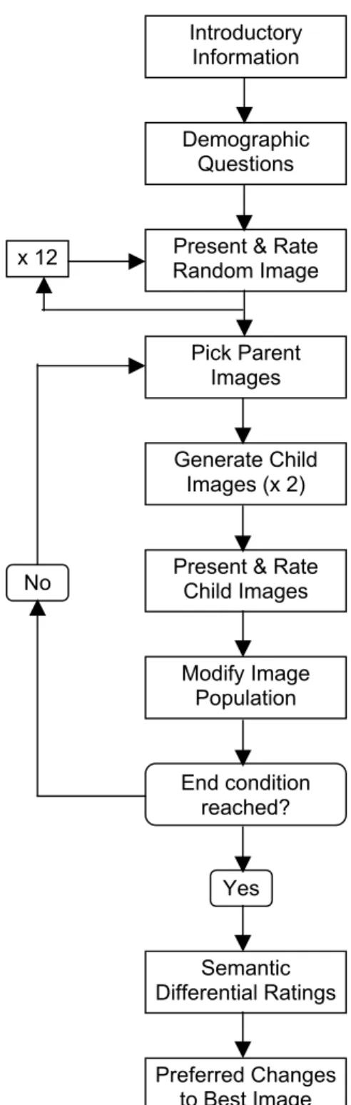
Software was written to present the images, to conduct the image manipulation according to the genetic algorithm, to administer
questionnaires, and to store data. A flow diagram is shown in Figure 3. Participants saw an initial set of 12 images, and rated each one for attractiveness, on a scale of 1 to 10. Images were presented one at a time, separated by 10 seconds when the screen was blank. Ten of the initial 12 images were random combinations of luminaire outputs, and were therefore different for every participant. The other two images were the same for all participants: an image with all luminaires at maximum output, and an image with all luminaires at a low (non-zero) output (labelled ‘Maximum’ and ‘Minimum’ in Figure 4). These images were randomly ordered within the other 10, and were included to give an early indication of the range of possible luminances. This set of 12 formed the initial “population” of images. Then the genetic algorithm process began.
2.2.2 The genetic algorithm
The algorithm was designed to mimic the process of Darwinian evolution. “Parent” images were selected from the population. One parent was the image with the highest attractiveness rating. The second parent was selected randomly from the population, but selection was weighted
according to the image’s attractiveness rating. These parent images “reproduced”, creating “child” images, and passing on successful “genes”. To describe the process mathematically, first we define “genes” for an image. We had four groups of luminaires each of which had 32 possible levels of output, arranged between 0 to 100%. In binary terms, the output of each luminaire group varied between 00000 and 11111 (i.e., between 0 and 31 in decimal terms). For example, an output level of 9 (or ~29% of full output) was represented by the gene 01001, a level of 22 (or ~71% of full output) by 10110, and so on. Five binary digits for each of four
luminaire groups resulted in a 20-digit binary string, or “phenotype” uniquely representing the luminaire outputs in a particular image (see Figure 4 for examples).
We mimicked sexual reproduction with operations on the binary strings called crossover and mutation (see Figure 5). The two parents (the “father” and the “mother”) produced two offspring (the “son” and the “daughter”). To create the son’s phenotype, we started with the first binary digit in the father’s phenotype. For each digit, reading from left to right, we randomly tested to see if crossover occurred, if it did not, the son’s digit was a copy of his father’s and the next digit of the father’s phenotype was tested. If crossover did occur the son’s digit was a copy of his mother’s and the next digit of the mother’s phenotype was tested. The possibility of crossover at each digit was set at 25%.
We also included random mutation, which could create gene combinations which otherwise would not occur. The possibility of mutation at each digit was set at 4%. The daughter was created in the same way as the son, except the process began with the mother’s phenotype.
An extra element was introduced to help the participant guide the genetic process – they indicated for each of four surfaces in an image whether they preferred it brighter, the same, or darker. The interface is shown in Figure 1. Because participants were unfamiliar with lighting technology, we articulated the luminaire outputs in terms of surface brightness.
Therefore Undershelf brightness preference affected the output of the task light; Ceiling brightness preference affected the direct/indirect up
component; Desk brightness preference affected the direct/indirect down component; and Far Walls brightness preference affected the wall
washers. The image did not change directly with these preferences, but when the next child was created, it was checked against the participant’s
brightness preference for each surface. If the child did not meet the set of preferences it was rejected and another child created and tested, until a satisfactory child was created. The approach of guiding the genetic process can increase the efficiency of a genetic algorithm [Caldwell & Johnston, 1991].
The children were then presented to the participant and rated for attractiveness. If they were rated more highly than the lowest rated images in the existing image population then they replaced these images, otherwise they were discarded. The process of parent selection and child creation continued until one of three end conditions was reached:
• An image received an attractiveness rating of 10;
• A participant preferred no brightness changes for all four surfaces;
• Neither of the latest two child images were rated more highly than the least attractive member of the existing population.
2.2.3 Semantic differential ratings
After the end condition was reached, participants rated the appearance of six images on a series of semantic differential (adjective pair) scales. Two of the images rated were the image with the highest attractiveness rating in the final population (Best image), and the image rated third highest from the initial population (75th percentile image), both of which were
(potentially) different for every participant. The other four images rated were identical for all participants. These were the Maximum and Minimum images described above, an image designed to give similar, mid-range, luminances on all surfaces (Neutral image), and an image designed to have the same overall luminance as the Neutral image but with higher luminance on the ceiling and far walls (Ceiling Boost image). These latter four images are shown in Figure 4.
Newsham et al. [2004] used 15 adjective pairs for semantic differential ratings. Factor analysis of their data suggested three basic factors related to attractiveness, uniformity, and brightness. We wanted to keep the time required of each participant to 30 minutes, so we used only nine individual rating scales in the present study. These nine scales were made up of three sets of three, each set designed to load on factors of Attraction, Non-Uniformity1, and Brightness. The three Attraction scales were: ugly –
1
This label is expressed in this way because higher values of the final variable indicated more variability, whereas lower values indicated uniformity.
beautiful; pleasant – unpleasant; comfortable – uncomfortable. The three
Non-Uniformity scales were: varied – unvaried; simple – complex;
non-uniform – non-uniform. The three Brightness scales were: bright – dim; dark – light; radiant – murky. The six images were presented in random order,
with each adjective pair presented one at a time next to the image. Participants gave their rating by moving a cursor on a continuous scale between the two adjectives; the value recorded ranged from 0 to 100. Finally, the Best image was recalled to the screen and the participant was asked to indicate, for each surface in turn, whether they would prefer it to be A lot Brighter, a little Brighter, No Change, a little Darker, or A lot Darker. The image did not change in response to this input.
Completion of the on-screen part of the experimental procedure took a mean time of 19:12 (min:sec); s.d. = 5:53.
2.2.4 A note on image rendering
Four lighting circuits each with 32 levels of output means 324 , or 1.05 million possible unique images. Rendering high quality images
on-demand, or pre-rendering all of the images in advance were not possible. Instead, we rendered all combinations of light output from the four circuits at four levels: 0, 33, 67 and 100% of full output, which gave 256 images. We then devised an interpolation scheme to generate any other possible combination of luminaire outputs from these 256 images in less than 10 seconds with low error (more information on this process is available at:
http://irc.nrc-cnrc.gc.ca/ie/lighting/office/images_e.html).
2.3 The Experimental Space
Images were projected onto a viewing screen using an InFocus LP530 data projector (see Figure 6). Participants sat in a chair and viewed the image through a height-adjustable rectangular slot. The inside of the space was completely black except for the image. The participant had access to a keyboard and a mouse for questionnaires and ratings. The distance from the projector to the viewing screen affected both the size of the image and the maximum brightness of the image. We chose a distance that gave an image that was 1.30m (51”) wide and 0.83m (33”) high; the computer monitor in the image was 0.125m (5”) corner to corner,
or about 33% of full size. Luminances in the image were then up to ~140 cd/m2, a typical maximum for most surfaces in a non-daylit office.
2.4 Luminance Measurements
To calibrate the display we projected a target onto the screen with five blocks of uniform grey, and measured their luminance values used a Topcon BM3 luminance meter. We adjusted the brightness and contrast settings on the projector to get a condition where the 0 grey level (“black”) was close to 0 cd/m2, the 255 grey level (“white”) was close to a typical maximum luminance, and the relationship between grey level and
luminance was close to linear in the most common luminance range (20 – 80 cd/m2). The final calibration is shown in Figure 7.
With the brightness and contrast levels fixed, we made the same
calibration measurements prior to each participant’s experimental session. These measurements are also shown in Figure 7. These data show that the projector’s output was not constant between sessions, and could vary by 10 – 15%. This seemed to be part of normal projector functioning. This effect does create error in the experimental process. However, the effect was largest at the high end of possible luminances, which were not achieved very often (only 24% of the Maximum image area was greater than 80 cd/m2), and were much smaller than the possible luminance range created by lighting circuit output settings.
After the experimental sessions were completed, the Best and 75th
percentile images for each of the participants, as well as the Maximum, Minimum, Neutral, and Ceiling Boost images, were re-projected in a
different laboratory. These images were measured using a Radiant Imaging Prometric video photometer, which took a digital picture of these stimuli and provided a luminance measurement for every pixel.
3. RESULTS & DISCUSSION
3.1 Did the Genetic Algorithm Lead to a Highly-Rated Image?
The mean attractiveness rating of the Best image (scale of 1 to 10) was 8.6 (s.d. = 1.3), and the modal rating was 9. When offered the opportunity to express a final preference in surface brightnesses of their Best image, 44% of the 160 votes (4 surfaces x 40 participants) were for ‘No Change’, and 89% for the three middle categories of ‘No Change’, ‘A little darker’ or
‘A little brighter’. A large majority of those wanting change preferred an increase in brightness, and preferences for change were not evenly distributed by room surface. For example, the number of participants wanting no change to the desk brightness was low; on the other hand, satisfaction with the brightness of the perimeter was high, with few people wanting change.
A measure of the efficiency of the algorithm is the number of images seen by the participants. Five participants gave an attractiveness rating of 10 to one of the 12 images in the initial population. The mean number of
images seen was 21.7 (s.d. = 10.3), small compared to the number of possible images.
Although the Best image was not perfectly optimal, it was rated very highly. Participants were viewing an image of a relatively uninspiring office space, and some might not have given a rating of 10 in any
circumstances. The Best image was achieved after viewing relatively few images. However, many participants desired further small brightness changes to their final Best image, particularly an increase in desk
brightness. The mean dimmer setting for the downward component of the direct/indirect fixtures, the circuit that most affected the desktop, was only 56%. This suggest that the optimization process did not allow participants to achieve high desktop brightness without compromising other
preferences. Therefore, there is room for improvement.
3.2 Are the Optimal (Best) Images Rated Differently than Non-Optimal Images?
We explored this was through the semantic differential appearance ratings of the images. Figure 8 shows the mean ratings for the six images for each of the adjective pairs. The mean brightness-related ratings for the
Maximum image are close to 100, and for the Minimum image are close to
0, therefore including the Maximum and Minimum images in the initial population to establish a brightness scale was successful. The Neutral and Ceiling Boost images were designed to have the same overall luminance, and their mean brightness-related ratings are very similar. Also as expected, the Best image has the highest mean scores on the attraction-related ratings (ugly – beautiful, unpleasant – pleasant,
Our plan was to reduce these nine ratings to the three concepts related to Attraction, Non-Uniformity, and Brightness. It is clear from Figure 16 that the mean values of ratings related to Attraction and Brightness were very consistent. It is equally clear that the scales intended to relate to Non-Uniformity neither agree with each other, nor discriminate very well between the six images2. The single scale uniform-non-uniform does order the mean ratings in the expected manner: the Minimum, Maximum, and Neutral images are the most uniform, and the Ceiling Boost image is the least uniform. Therefore, for further statistical tests, our measure of Non-Uniformity was the single item rating uniform – non-uniform.
Descriptive statistics for the three scales are shown in Table 2.
We conducted statistical analyses on these three subjective outcomes to test differences between the images. There were a priori reasons for the following comparisons:
• Best vs. Neutral – a test of whether optimal images differed in
ratings from another image, in this case the comparison is to a non-optimal, “average” image;
• Best vs. 75th percentile – a more rigorous test of whether optimal
images differed in ratings from another image, in this case the comparison is to a non-optimal, but relatively attractive image;
• Best vs. Maximum – previous research [Newsham et al., 2004]
suggested that brighter images were more attractive; this comparison tests whether the optimal image, which is not
maximally bright, differs in ratings from the maximally bright image;
• Neutral vs. Ceiling Boost – previous research [Newsham et al.,
2004] suggested that brighter ceilings were more attractive; this comparison tests whether images with the same brightness overall differ in ratings when the ceiling is brighter in one of the images. We first conducted overall multivariate analyses of variance (MANOVA) for the planned comparisons to test for an overall difference across
outcomes. It is usual practice (to control for Type I statistical errors) to test for univariate differences (differences on single outcomes) only if the overall MANOVA is significant. Only two of the planned comparisons had significant MANOVAs; the results of the tests are shown in Table 3. The Best image was rated significantly brighter and more attractive than the Neutral image, as expected. On average, the Best image had higher
2
luminance (see Table 4): 36.9 cd/m2 vs. 28.4 cd/m2. The Best image was rated significantly less bright than the Maximum image, and the Maximum image had a higher luminance (55.6 cd/m2). Nevertheless, the Best image was significantly more attractive than the Maximum image, suggesting that images that are too bright are less attractive. Previous research
[Newsham et al., 2004] suggested that images that are too uniform are also less attractive, and the Maximum image was rated as significantly more uniform than the Best image.
There was no significant difference between the Best and 75th percentile
images on the room appearance ratings. There was little difference between the images in luminance (75th percentile image mean was 35.6
cd/m2). Note that the ratings of image attractiveness made on a scale of 1 – 10 used during the optimization process did differ significantly between the two images (Best: Mean=8.6, s.d. 1.3; 75th percentile: Mean=6.6, s.d.
1.5; F(1,39)=69.98, p<0.001, η2 partial = 0.64). In Newsham et al. [2004]
the 75th percentile image was much less realistic than the Best image, and
there were significant differences in room appearance ratings. Perhaps the use of more realistic images meant the range of appealing images was wider.
The MANOVA showed no significant difference in ratings between the
Neutral and Ceiling Boost images. Therefore the finding of our previous
work, which indicated the primacy of ceiling luminance in determining attractiveness, was not supported. This could have been because the images were both too dim, or because we did not boost the ceiling luminance enough in the Ceiling Boost image.
3.3 Are Preferred Luminances the same as Those Derived from Experiments in Real Spaces?
Table 4 presents a summary of the luminance information from the images, and Figure 9 shows how the image was divided into surfaces for analysis. Table 4 also contains a physical measure of image luminance non-uniformity, labelled RMS, calculated as follows:
RMS =
√
(
∑i ((Lumi – WAV) 2• Ni) / (∑i Ni) • WAV
)
where,
i = surface label for 1 to 9 surfaces Lumi = mean luminance of surface i (cd/m2)
WAV = weighted average luminance of image (cd/m2) Ni = number of data points (relative area) for surface i
RMS accounts for the difference between the individual surface
luminances and mean luminance. It is scaled by the mean luminance, so that images do not have higher values just by virtue of being brighter. The higher the value of RMS the higher the physical non-uniformity.
We compared the preferred luminous conditions in the Best images to those derived from experiments in real spaces. All of the studies we refer to in this section excluded daylight, analogous with our study.
Loe et al. [1994] had observers rate a small conference room from a point equivalent to the room’s entrance. Lighting conditions were manipulated by the experimenters using a variety of luminaires. They concluded that for ‘visual lightness’ the preferred average luminance in a horizontal band 40o wide should be >= 30 cd/m2. We have approximated an equivalent average luminance, shown in Table 4 with the label ’40-deg band’. This is the weighted mean luminance of the far walls, other cubicles, partitions, desk, and computer screen. The median value in the Best images was 37.7 cd/m2, and only 9 participants chose Best images with the 40-deg band luminance below 30 cd/m2.
Veitch and Newsham [2000] conducted a study in a similar workstation in a laboratory. Participants had dimmable control over three lighting circuits (one indirect and two direct) as well as on-off control over an undershelf task light. Participants occupied the space for an 8-hour day and
conducted typical office tasks. One value reported was the mean
luminance in an area that included the partitions behind the computer and under a binder bin, part of the desktop and part of the binder bin – chosen to represent the 40o horizontal band of field of view from Loe et al. [1994]. The median luminance in this area resulting from participants’ choices was 39.2 cd/m2 (min. = 11.5, max. = 61.0). The median luminance of the partitions and 40-deg band in the Best images was 35.5 cd/m2 (min. = 12.3, max. = 55.9), and 37.7 cd/m2 respectively.
Berrutto et al. [1997] gave participants dimming control over various luminaires in small private offices. Exposures were limited to 20 minutes, and data were collected separately for different tasks. They concluded that for non-VDT tasks wall luminance at eye level should be around 60-65 cd/m2, and for VDT tasks the luminances around the screen should be
equal or lower than the luminance of the screen. In our study, the median screen luminance in the Best images was 30.6 cd/m2 and the partitions had a median luminance of 35.5 cd/m2.
Van Ooyen et al. [1987] presented participants with different office luminous environments by manipulating light distributions and changing the reflectivity of surfaces; working plane illuminance was maintained at around 750 lux. The spaces were private two-person offices, and data were collected separately for different tasks. For non-VDT tasks, preferred wall luminances were 30 to 60 cd/m2, and preferred working plane luminances were 45 to 105 cd/m2. For VDT work the values were reduced: preferred wall luminances were 20 to 45 cd/m2, and preferred working plane luminances were 40 to 65 cd/m2. In our study, the median partition luminance of the Best images was 35.5 cd/m2, and the median desktop luminance was 52.5 cd/m2. Van Ooyen et al. reported that the preferred ratio of working plane luminance to wall luminance was 1.33. In our study, the equivalent ratio, desk:partitions, was 1.49. Note that with the lighting systems we modelled, a low desk:partition ratio was very difficult to achieve.
Finally, we looked at the variability in individual preference. We observed a wide variety of preferred luminances in the Best images. This is
encouraging because studies of individual preference in real spaces also report wide variety. We performed a quantitative comparison to the results of Veitch and Newsham [2000]. Figure 10 shows a plot of two measures of the frequency of preferred luminance: for Veitch and Newsham we plot the mean luminance in the (approx.) 40o horizontal band of field of view (as described above). For this study, we plotted the derived value labelled ’40-deg band’ in Table 4. The two curves show remarkable agreement.
Taken together, these comparisons show that the preferred luminances derived from our study compare well with the preferred luminances from studies in real spaces. As such, these comparisons reinforce the
hypothesis that the images are perceived in the same way as real spaces.
3.4 Do Subjective Ratings Correlate with Photometric Descriptors?
Lighting researchers have often sought to correlate occupant ratings of luminous environments with photometric descriptors. This task has
et al., 1979; Loe et al., 1994; Veitch & Newsham, 1998; Newsham & Veitch, 2001].
Therefore we examined whether photometric measures of the images (such as those in Table 4) were predictive of Attraction, Non-Uniformity, and Brightness ratings, using linear regressions. We began by including ratings and photometric values for all six images rated using the semantic differential scales. This gave us 240 data points per regression (6 images x 40 participants). Because each participant provided six data points, the points are not independent and simple regressions would provide
misleading results. Two of the six images varied between participants, making traditional analysis-of-variance techniques inappropriate. The relatively new statistical technique of Hierarchical Linear Modelling (HLM, or mixed regression) [Bryk & Raudenbush, 1992; Hox, 1995] accounts for the within-subject effects in this kind of analysis. Conceptually, this
analysis consists of creating separate regression lines for each participant, and then testing the distribution of regression weights (slopes and
intercepts) against the null hypothesis that the average regression weight equals zero. The technique also produces a single best-fit regression line across all data points3. The results of the HLM analyses are summarized in Table 5.
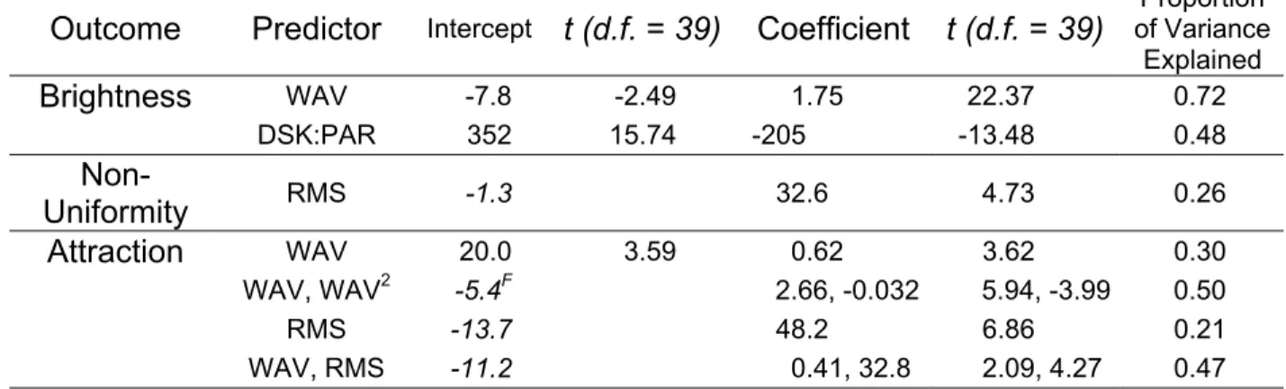
We expected that images with a higher average luminance (labelled ‘WAV’ in Table 5) would have higher Brightness ratings. The HLM analysis showed the linear trend was significant, and the proportion of variance explained was high (0.72). Note that the intercept was close to the origin, as expected: an image with a luminance of zero should get a zero rating of Brightness.
We were concerned that the linear relationship between Brightness and WAV was being driven by ratings of images at the extremes of the luminance range: the Minimum and Maximum images. We therefore repeated the analysis with these images removed. The linear trend was still significant and strong, with coefficients similar to those from the analysis with all six images: intercept = -6.8; slope = 1.71 (t = 8.59, d.f. = 39, p < 0.001); proportion of variance explained = 0.51. Similarly, in the
3
The model we generally used was a random intercept and random slope model with no centering, with one or more photometric predictors at level-1, and no level-2 predictors; we were interested in explaining whether photometric variables predicted appearance ratings (level-1), and not in investigating what participant characteristics might have led to differences in ratings between participants (level-2).
analyses of Uniformity and Attraction below, we found that removing the data from the Minimum and Maximum images did not substantially affect the results. Therefore, all analyses in Table 5 include data from all six images.
The weighted average luminance was highly correlated (r > 0.85) with all the other luminances shown in Table 4. This is almost inevitable with real lighting systems. We did repeat the HLM analysis on Brightness ratings using the other luminances as predictors, but found that all were very similar in predictive power. Therefore, we conducted other analyses with WAV as the luminance predictor.
Previous work using the genetic algorithm method [Newsham et al., 2004], and using brightness matching and rating scales methods in real spaces [Tiller & Veitch, 1995; Tiller et al., 1995] found a significant relationship between ratings of brightness and photometric uniformity: less uniform images were rated as being more bright. Data from this study supported this. Table 5 shows a significant relationship between Brightness rating and RMS, with a positive slope. However, using WAV and RMS together as predictors of Brightness ratings did not increase the predictive power over using WAV alone. WAV and RMS are correlated (r = 0.37), with more luminous images tending to be less uniform. The relationship between Brightness and RMS might have resulted from this confound, although this seems unlikely given that the relationship between brightness and uniformity was observed in two experiments in which uniformity varied while average luminance was held constant [Tiller & Veitch, 1995; Tiller et al., 1995].
We also found a significant relationship between Brightness rating and the ratio between desk and partition luminance (labelled DSK:PAR in Table 5). The slope was negative, indicating that the lower the luminance difference between these two surfaces the higher the Brightness rating. However, using WAV and DSK:PAR together as predictors of Brightness ratings did not increase the predictive power over using WAV alone. WAV and DSK:PAR were highly correlated (r = -0.83), with more luminous images tending to feature desks and partitions with more similar
luminances. The relationship between Brightness and DSK:PAR might have resulted from this confound.
For Non-Uniformity, the obvious first predictor was RMS. The relationship between Non-Uniformity ratings and RMS was significant and in the
expected direction. The intercept was very close to zero, as expected: an image where all surfaces had the same mean luminance should be
subjectively rated as very uniform. This result supports the relationship found in Newsham et al. [2004], but is not as strong. This is likely
because in the previous work the range of photometric variability between images was much larger.
Whereas there were obvious photometric predictors for ratings of
Brightness and Non-Uniformity, there were no such obvious predictors for ratings of Attraction. Newsham et al. [2004] showed that brighter images were rated as more attractive, so we began there. Table 5 shows that the relationship was significant, WAV explained 30% of the variance in
Attraction ratings. Figure 8 suggests that the relationship with WAV was not linear, the Maximum images received lower average attractiveness-related ratings then the Best images, despite having a higher average luminance. This implies a quadratic component to the relationship, and therefore we examined Attraction vs. WAV and WAV2. This relationship was also significant, and explained 50% of the variance in Attraction ratings, substantially more than WAV alone. The coefficients were also in the expected direction: positive for WAV so that Attraction increases with luminance at low luminances, and negative for WAV2, resulting in a penalty on Attraction if average luminance is too high.
Newsham et al. [2004] also suggested that some non-uniformity increased attractiveness, but excessive non-uniformity decreased attractiveness. Therefore, we examined the Attraction vs. RMS relationship. The relationship was significant with a positive coefficient, the more non-uniform the image, then more attractive it was rated. To test if excessive non-uniformity was negative for attractiveness, we examined Attraction vs. RMS and RMS2. This relationship explained 27% of the variance in
Attraction ratings, a little more than RMS alone. The coefficients were also in the expected direction: positive for RMS so that Attraction increased with non-uniformity at low non-uniformity, and negative for RMS2, resulting in a penalty on Attraction if non-uniformity was too high. However, although the RMS coefficient was significant, the RMS2
coefficient just failed the significance test (p = 0.059). Normally we do not comment on non-significant tests (and this test is not included in Table 5), but we comment here because of the theoretical interest in this trend. The lighting design we used to create the images did not generate a large range of values photometric uniformity. Images with more variability might produce a significant Attraction vs. RMS and RMS2.
As noted above, WAV and RMS are positively correlated, and it could be that the significant relationship between Attraction and RMS arose
because images with higher RMS values also tended to be brighter. Therefore we examined Attraction vs. WAV and RMS. Table 5 shows that this relationship was significant, and explained 47% of the variance in Attraction ratings, substantially more that either WAV or RMS alone. This result suggests that RMS is contributing unique explanatory power.
The obvious next step would be try WAV, WAV2 and RMS together as predictors. Unfortunately, given the data we had, the HLM analyses were not stable for three predictors. Future studies with more participants observing more images might allow for HLM analyses with more predictors.
The models of Attraction vs. WAV and WAV2, and Attraction vs. WAV and RMS both explained about the same proportion of variance. We
encourage others to explore these relationships in future studies, both with images and with real spaces as stimuli. We also recommend ensuring a wider range for the photometric predictor values.
4. CONCLUSIONS
The general goal of this experiment – to replicate and extend the findings of Newsham et al. [2004] using a more realistic image – was met. The results demonstrated that the genetic algorithm approach was quite successful in obtaining a participant’s preferred luminance patterns in a high-quality, realistic colour image of an office space. Further, the
preferred luminances from the projected images were very similar to those from experiments conducted in real settings.
Importantly for lighting quality research, subjective ratings of room appearance in the image were significantly related to photometric
descriptors of the image. Ratings of image brightness were predicted by the average luminance of the image (WAV), and by a measure of
photometric non-uniformity (RMS). Ratings of image non-uniformity were predicted by RMS. And, in particular, ratings of image attractiveness were predicted by various combinations of WAV, WAV2, RMS, and RMS2. The latter result indicates that an attractive image of an office space is one that is bright, but not too bright, and that has some non-uniformity but is not too non-uniform.
Our results suggest that evaluation of images has value as both a research tool and a method of presenting lighting design solutions to clients and occupants. If future work reinforces our findings that image evaluation is equivalent in many ways to the aesthetic evaluation of real spaces, this method might, in some circumstances, be able to replace much more expensive studies in real settings.
5. ACKNOWLEDGEMENTS
This work was sponsored by the National Research Council Canada (NRC), the Program for Energy Research & Development (PERD), and Public Works & Government Services Canada (PWGSC). The work was conducted under the PERD Lighting and Daylighting Project “Energy-efficient lighting and daylighting design in the modern workplace: defining occupant preference and increasing occupant performance”, as part of the NRC/PWGSC Agreement “Lighting for VDT workstations: preferences and energy-efficient solutions” (NRC Project Number B3208). The authors are grateful for the technical help provided by Roger Marchand (NRC), Jana Svec (NRC), and Anca Galasiu (NRC). Thanks are also due for the support of Morad Atif (NRC), Ivan Pasini (PWGSC) and Karen Pero (PWGSC). We are also grateful to our NRC colleagues who volunteered to participate in this experiment.
6. REFERENCES
Ashdown, I. 1994. “Non-imaging optics design using genetic algorithms”,
Journal of the Illuminating Engineering Society, Winter, pp. 12-21.
Berrutto, V.; Fontoynont, M.; Avouac-Bastie, P. 1997. “Importance of wall luminance on users satisfaction: pilot study on 73 office workers”.
Proceedings of Lux Europa – 8th European Lighting Conference (Amsterdam), pp. 82-101. NSVV (Arnhem).
Bishop, I.D.; Rohrmann, B. 2002. "Subjective responses to simulated and real environments: a comparison," Landscape and Urban Planning, 65, pp. 261-277.
Bryk, A.S.; Raudenbush, S.W. 1992. Hierarchical Linear Models, Sage Publications (Newbury Park, CA, USA).
Caldwell, C.; Johnston, V.S. 1991. “Tracking a criminal suspect through ‘Face-Space’ with a genetic algorithm”, Proceedings of the 4th
International Conference on Genetic Algorithms (San Diego), pp. 416-421. Morgan Kaufmann (San Mateo).
Chutarat, A.; Norford, L.K. 2001. “A new design process using an inverse method: a genetic algorithm for daylighting design”, Proceedings of IESNA Annual Conference (Ottawa), pp. 217-229. Illuminating Engineering
Society of North America (New York).
Corcione, M.; Fontana, L. 2003. “Optimal design of outdoor lighting
systems by genetic algorithms,” Lighting Research and Technology 35(3), pp. 261 – 280.
Danford, S.; Willems, E.P. 1975. “Subjective responses to architectural displays,” Environment and Behavior 7(4), pp. 486-516.
Daniel, T.C.; Meitner, M.M. 2000. “Representational validity of landscape visualizations: the effects of graphic realism on perceived scenic beauty of forest vistas,” Journal of Environmental Psychology 21, pp. 61-72.
Eklund, N.H.; Embrechts, M.J. 2001. “Multi-objective optimization of spectra using genetic algorithms”, Journal of the Illuminating Engineering
Society, Summer, pp. 65-72.
Flynn, J.E.; Hendrick, C.; Spencer, T.; Martyniuk. 1979. “A guide to
methodology procedures for measuring subjective impressions in lighting”.
Journal of the Illuminating Engineering Society, 8 (2), pp. 95 - 110.
Hendrick, C.; Martyniuk, O.; Spencer, T.J.; Flynn, J.E. 1977. “Procedures for investigating the effect of light on impression: simulation of a real space by slides,” Environment and Behavior 9 (4), pp. 491-510.
Hox, J.J. 1995. Applied Multilevel Analysis, TT-Publikaties (Amsterdam, The Netherlands).
Johnston, V.S. 1999. Why We Feel, Perseus Books (Reading, MA, USA).
Johnston, V.S.; Franklin, M. 1993. “Is beauty in the eye of the beholder?,” Ethology and Sociobiology 14, pp. 183-199.
Kawai, J.K.; Painter, J.S.; Cohen, M.F. 1993. “Radioptimization - goal based rendering”, Proceedings of SIGGRAPH (Anaheim), pp.147-154. Loe, D. L.; Mansfield, K. P.; Rowlands, E. 1994. “Appearance of lit environment and its relevance in lighting design: experimental study,”
Lighting Research and Technology 26(3), pp. 119 – 133.
Mahdavi, A.; Eissa, H. 2002. “Subjective evaluation of architectural lighting via computationally rendered images,” Journal of the Illuminating
Engineering Society, 31(2), pp 11-20.
Moeck, M. 2001. “Designed appearance lighting - revisited”, Journal of
the Illuminating Engineering Society, Summer, pp. 53-64.
Newsham, G.R.; Veitch, J.A. 2001. "Lighting quality recommendations for VDT offices: a new method of derivation," Lighting Research and
Technology, 33 (2), pp. 97-116.
Newsham, G.R.; Marchand, R.G.; Veitch, J.A. 2004. “Preferred surface luminances in offices, by evolution”, Journal of the Illuminating
Engineering Society, 33 (1), Winter, pp. 14-29.
Rohrmann, B.; Bishop, I. 2002. "Subjective responses to computer
simulations of urban environments," Journal of Environmental Psychology,
22, pp. 319-331.
Schoeneman, C.; Dorsey, J.; Smits, B.; Arvo, J.; Greenberg, D. 1993. “Painting with light”, Proceedings of SIGGRAPH (Anaheim), pp.143-146. Tiller, D. K., & Veitch, J. A. 1995. Perceived room brightness: Pilot study on the effect of luminance distribution. Lighting Research and Technology,
27, 93-101.
Tiller, D. K., Veitch, J. A., & Pasini, I. C. 1995. The effects of luminance distribution on perceived room brightness. In Proceedings of the
Commission Internationale de l’Éclairage 23rd Session, New Delhi, India, November 1-8, 1995 (CIE 119-1995, Vol. 1, pp. 144-147). Vienna,
Van Ooyen, M.H.F.; van de Weijgert, J.A.C; Begemann, S.H.A. 1987. “Preferred luminances in offices”. Journal of the Illuminating Engineering
Society, Summer, pp. 152 - 156.
Veitch, J.A.; Newsham, G.R. 1998. “Lighting quality and energy-efficiency effects on task performance, mood, health, satisfaction and comfort”. Journal of the Illuminating Engineering Society, Winter, pp. 107 - 129.
Veitch, J.A.; Newsham, G.R. 2000. “Preferred luminous conditions in open-plan offices: research and practice recommendations”, Lighting
Table 1. Participant characteristics.
Total responses
Sex Female Male
40 28 12
Age 18-29 30-39 40-49 50-59 60-69
40 2 9 16 13 0
Correction
Lenses None Reading Glasses Distance Glasses Bi- or Trifocal Lenses Gradual or Multifocal Lenses Contact Lenses 40 10 3 12 8 5 2 Principal
Occupation Administrative Technical Professional Managerial
40 22 0 15 3
Language English French
Table 2. Descriptive statistics for the three scales used in statistical tests.
Attraction Non-Uniformity Brightness Image
(ugly – beautiful, unpleasant – pleasant, uncomfortable – comfortable)
(uniform – non-uniform) (dim – bright, dark – light, murky – radiant) Best Min. 0.0 0.0 6.0 Max. 100.0 100.0 100.0 Med. 67.8 39.5 57.8 M 63.8 42.6 58.1 SD 26.2 28.6 24.7 75th percent Min. 0.0 0.0 5.3 Max. 100.0 100.0 100.0 Med. 53.0 49.0 49.7 M 53.3 41.4 55.6 SD 29.2 28.1 29.0 Neutral Min. 0.0 0.0 0.0 Max. 88.0 80.0 100.0 Med. 36.3 40.5 38.3 M 39.8 36.6 41.3 SD 25.4 22.0 27.3 Ceiling Bst. Min. 0.0 0.0 0.0 Max. 100.0 100.0 91.7 Med. 34.5 50.0 35.0 M 37.5 45.0 41.2 SD 24.4 27.6 26.5 Maximum Min. 0.0 0.0 0.0 Max. 100.0 97.0 100.0 Med. 28.7 20.5 94.3 M 41.4 25.4 89.6 SD 37.4 26.4 13.6 Minimum Min. 0.0 0.0 0.0 Max. 85.7 92.0 34.3 Med. 5.3 10.5 1.7 M 11.8 24.2 5.1 SD 19.9 27.8 7.6
Table 3. Result of MANOVAs and univariate effects on appearance ratings. Statistical tests were within-subjects on a single independent variable: image type; with two levels in each comparison. Only statistically
significant effects are shown (p < 0.01). η2 partial is a measure of effect size, or proportion of variance explained by the effect.
Best vs. Neutral Best vs. Maximum
Outcome F(1,39) η2 partial F(1,39) η2 partial
Attraction 28.24 0.42 9.76 0.20 Non-Uniformity 7.98 0.17 Brightness 9.68 0.20 55.79 0.59 MANOVA: Wilks’ Λ = 0.528; η2 partial(ave) = 0.22; F(3,37) = 11.01 MANOVA: Wilks’ Λ = 0.362; η2 partial(ave) = 0.32; F(3,37) = 21.69
Table 4. Luminance-related information for the six different images (cd/m2). Values from the Best and 75th percentile images were different
for each of the 40 participants, therefore measures of variability are shown. Values for the Neutral, Ceiling boost, Maximum and Minimum images were the same (within experimental error) for every participant. Values for combinations of surfaces were calculated by weighting each
surface’s contribution according to its size.
Best image Min. Max. Median Mean s.d.
Ceiling 7.9 57.5 40.5 37.5 14.3 Far walls 13.6 62.4 42.1 39.8 14.2 Other cubicles 12.4 54.0 32.1 32.9 11.7 Left partitions 9.3 54.4 34.7 34.4 11.4 Left desk 15.2 74.1 55.3 53.3 14.3 Right partitions 10.5 57.0 33.9 34.5 12.9 Right desk 12.6 73.5 50.2 48.5 16.5 Computer Screen 17.5 43.3 30.6 30.3 7.0
Other Image Areas 14.0 45.4 31.1 30.3 8.6
Weighted Average 13.8 57.4 36.6 36.9 11.7
Left partitions + Left desk 11.2 60.7 41.0 40.4 12.2
Right partitions + Right desk 11.3 63.0 39.4 39.5 14.1
Left partitions + Right partitions 12.3 55.9 35.5 34.4 11.9
Left desk + Right desk 19.9 73.8 52.5 50.3 14.6
40-deg band 14.7 60.2 37.7 38.3 12.3
Desk : Partitions 1.32 1.76 1.49 1.50 0.11
Table 4. continued …
75th percentile image Min. Max. Median Mean s.d.
Ceiling 7.2 52.6 44.4 38.1 13.5 Far walls 9.6 56.7 45.0 39.0 15.1 Other cubicles 6.9 48.6 33.9 31.7 10.4 Left partitions 4.7 49.4 33.8 31.5 10.4 Left desk 7.3 68.6 52.8 49.2 15.2 Right partitions 6.8 50.7 33.8 32.8 11.0 Right desk 10.4 68.8 50.1 47.0 14.7 Computer Screen 14.2 38.4 29.9 29.4 5.9
Other Image Areas 9.5 41.3 29.9 29.2 7.6
Weighted Average 8.0 51.9 38.5 35.6 11.0
Left partitions + Left desk 5.5 55.6 39.8 37.1 11.9
Right partitions + Right desk 8.1 56.7 39.4 37.9 12.3
Left partitions + Right partitions 6.0 50.1 33.5 32.2 10.5
Left desk + Right desk 9.3 67.0 50.1 47.8 14.2
40-deg band 7.8 54.3 38.7 36.5 11.5 Desk : Partitions 1.34 1.76 1.48 1.50 0.09 RMS 0.7 1.7 1.2 1.2 0.2 Image Type Neutral Ceiling
Boost Maximum Minimum
Ceiling 29.4 38.0 56.8 7.4 Far walls 32.6 41.8 61.7 10.8 Other cubicles 25.6 26.2 52.5 7.0 Left partitions 20.7 19.9 51.5 4.8 Left desk 32.5 28.6 70.3 7.6 Right partitions 27.3 24.3 55.7 6.9 Right desk 41.9 33.9 71.6 10.8 Computer Screen 25.9 24.8 41.0 15.2
Other Image Areas 24.6 23.2 42.9 10.1
Weighted Average 28.4 29.1 55.6 8.2
Left partitions + Left desk 24.5 22.7 57.5 5.7
Right partitions + Right desk 32.6 27.8 61.4 8.3
Left partitions + Right partitions 24.5 22.4 53.9 6.0
Left desk + Right desk 38.3 31.9 71.1 9.6
40-deg band 29.0 28.3 58.3 7.9
Desk : Partitions 1.57 1.42 1.32 1.59
Table 5. Results of the HLM analyses. Each line shows a separate regression model, using the predictor variables indicated. All coefficients (slopes) shown are statistically significant (p < 0.05). All intercepts shown
were also are statistically significant (p < 0.05), unless shown in italics. WAV=Weighted Average Luminance; DSK:PAR=Desk:Partitions.
Outcome Predictor Intercept t (d.f. = 39) Coefficient t (d.f. = 39)
Proportion of Variance Explained Brightness WAV -7.8 -2.49 1.75 22.37 0.72 DSK:PAR 352 15.74 -205 -13.48 0.48 Non-Uniformity RMS -1.3 32.6 4.73 0.26 Attraction WAV 20.0 3.59 0.62 3.62 0.30 WAV, WAV2 -5.4F 2.66, -0.032 5.94, -3.99 0.50 RMS -13.7 48.2 6.86 0.21 WAV, RMS -11.2 0.41, 32.8 2.09, 4.27 0.47
Note, in this analysis the proportion of variance explained refers to variance at level-1, at the level of the individual ratings. The total variance at level-1 is calculated using a ‘random intercept model’ that is, an HLM model with no predictors; call this σ1
2
. We then add the level-1 photometric predictor, which reduces the unexplained level-1 variance to σ2
2
. The proportion of variance explained at level-1 is then (σ12 - σ22)/ σ12.
F
This is a fixed intercept model, meaning that when HLM calculates regression equations for each participant, it assigns each participant the same (best-fit) intercept. Our general preference is to use a non-fixed (random) intercept for our models, but this particular model is not stable without a fixed intercept.
Nevertheless, a fixed intercept, with a value close to zero, is not unreasonable in this case. With a luminance of zero it is a reasonable assumption that all
Figure 1. Interface for the experimental task. Participants rated the image
http:/ tml
for overall attractiveness on a scale of 0-10. They then used the boxes at the bottom to indicate their brightness preference for each surface.
Example images can be viewed in colour at:
3.5 ft 5 ft 10 ft 8 ft 7.4 ft 9.4 ft 34 ft 56 ft
Figure 2. A plan view of the model used for the LightscapeTM renderings. The suspended direct/indirect fixtures are clearly visible as the white
Preferred Changes to Best Image Modify Image Population No Yes End condition reached? Present & Rate
Child Images Generate Child
Images (x 2) Pick Parent
Images x 12 Present & Rate
Random Image Semantic Differential Ratings Demographic Questions Introductory Information
Figure 4. Four of the images used in the semantic differential ratings. Images are (from top left, clockwise): Maximum, Minimum, Ceiling Boost,
Father: 1 0 0 0 0 0 0 0 1 0 1 1 0 1 0 0 0 1 0 0 Mother: 0 0 0 0 0 0 0 1 0 1 1 1 0 1 0 1 0 1 1 1 Son: 1 0 00 0 0 0 11 0 01 0 1 0 0 0 11 1 Crossover occurs Crossover occurs Mutation occurs Crossover occurs
Figure 5. Crossover and mutation from parents’ phenotypes (lower two images in Figure 4) to create a son phenotype; mother’s genes are underlined. Resulting combination of
2.45m (96”)
viewport Projection screen
Computer LCD projector
3.24m (128”)
1.70m (67”)
3.73m (147”)
Figure 6. Experimental set-up. Participants viewed the projected image through a viewport (photo on left). The space into which they looked was
black except for the projected image. Diagram shows side elevation, approximately to scale.
0 20 40 60 80 100 120 140 160 180 0 64 128 192 256 Grey Level L u m in an ce ( c d /m 2 )
Figure 7. Calibration of projector screen luminance vs. image pixel grey level. Shown upper right is the image that was projected onto the screen to make the calibration measurements. Diamond symbols with heavy (red) line shows original calibration. Lighter lines show measurements made prior to each participant doing the experiment.
0 10 20 30 40 50 60 70 80 90 100 ugly unpl easa nt uncom fortab le unvar ied sim ple unifo rm dim dark murky M ean R a ti n g bea utifu l pleas ant com fortab le varied com plex non -uni form brigh t light radia nt Best 75th percentile Neutral Ceiling Boost Maximum Minimum
ugl-bea unp-ple unc-com unv-var sim-com uni-non dim-bri dar-lig mur-rad Image
30.0 26.5 26.8 27.1 27.7 28.6 28.5 28.6 22.4 Best 30.1 32.6 30.9 29.7 25.1 28.1 30.3 32.5 29.4 75th percentile 25.3 27.8 28.8 23.8 24.1 22.0 28.1 29.4 26.8 Neutral 25.7 27.7 24.4 26.3 26.9 27.6 27.8 29.3 26.5 Ceiling Boost 35.7 39.2 39.3 33.3 32.6 26.4 15.0 14.6 16.9 Maximum 17.0 21.1 23.5 19.5 35.6 27.8 6.8 7.0 12.0 Minimum Figure 8. Comparison of mean semantic differential appearance ratings
for the Best, 75th percentile, Neutral, Ceiling Boost, Maximum, and Minimum images. Table shows standard deviations associates with each
Surface Pixels Ceiling 623 Far walls 396 Other cubicles 502 Left partitions 437 Left desk 205 Right partitions 581 Right desk 330 Screen 42 Miscellaneous 592
Figure 9. How the image was divided into areas for luminance analyses. Also shown are the number of data points for each surface from the
0 10 20 30 40 10 20 30 40 50 60 70 n field of view (cd/m2) Fr e que nc y , % Real Space Images Brightness i Luminance
Figure 10. Preferred luminance in the field of view, for this study and a study done in a real space [Veitch & Newsham, 2000].