Crustal structure beneath broad-band seismic stations
in the Mediterranean region
Mark van der Meijde, Suzan van der Lee and Domenico Giardini
ETH Z¨urich faculty of geophysics, ETH H¨onggerberg (HPP), CH-8093 Z¨urich, Switzerland. E-mail: [email protected]
Accepted 2002 October 4. Received 2002 August 1; in original form 2001 December 04
S U M M A R Y
We have analysed receiver functions to derive simple models for crustal structure below 12 broad-band seismological stations from the MIDSEA project and 5 permanent broad-band stations in the Mediterranean region including northern Africa. To determine an accurate Moho depth we have reduced the trade-off between crustal velocities and discontinuity depth using a new grid search method, which is an extension of recently published methods to determine crustal thickness. In this method the best fitting synthetic receiver function, containing both the direct conversion and the reverberated phases, is identified on a model grid of varying Moho depth and varying Poisson’s ratio. The values we found for Moho depth range from around 20 km for intra-oceanic islands and extended continental margins to near 45 km in regions where the Eurasian and African continents have collided. More detailed waveform modelling shows that all receiver functions can be well fit using a 2- or 3-layer model containing a sedimentary layer and/or a mid-crustal discontinuity. On comparing our results with Moho maps inferred from interpolated reflection and refraction data, we find that for some regions the agreement between our receiver function analysis and existing Moho maps is very good, while for other regions our observations deviate from the interpolated map values and extend beyond the geographic bounds of these maps.
Key words: broad band, crustal structure, Moho discontinuity, Poisson’s ratio, seismic
deconvolution.
1 I N T R O D U C T I O N
The main tectonic feature in the Mediterranean region is the plate boundary between Eurasia and Africa. Plate motion in the region is dominated by slow convergence between the two plates, alter-nated with relatively rapid extension in subdomains within the region (Wortel & Spakman 2000). The convergence has resulted in zones of continental collision with thickened continental crust, such as the Dinarides (Dragaˇsevi´c & Andri´c 1968). Trench roll-back in the re-gions of subduction is thought to have led to the rapid opening of both the Tyrrhenian and Aegean basins and has significantly extended the continental crust of these basins (Meissner et al. 1987). The complex characteristics and tectonic evolution of the plate bound-ary are described in detail in e.g. Dercourt et al. (1986), Dewey
et al. (1989) and Jonge et al. (1994). This tectonic complexity of
the Mediterranean region is reflected in strong lateral variations in crustal structures.
A range of characteristic crustal types have been defined by Mooney et al. (1998) in their global compilation of crustal prop-erties. They characterized the crust of the entire Earth through 14 primary crustal types. Each crustal type was derived by calculating an average model based on seismic refraction profiles recorded in crust of specific age or tectonic setting. Half of these primary crustal
types are found in the Mediterranean alone, which comprises only 1.5 per cent of Earth’s surface.
A detailed map of crustal thicknesses in the Mediterranean re-gion is presented by Meissner et al. (1987) (Fig. 1). The contour map shows strong variations in the depth of the Mohoroviˇci`c dis-continuity (Moho) between the different tectonic subdomains in the Mediterranean. The Moho depth varies from less than 15 km for the extended crust in the Algero-Provencal Basin to more than 40 km under the Dinarides, Pyrenees and Alps. Several deep seis-mic sounding profiles and extensive reflection/refraction profiles have been shot in the Mediterranean and have been incorporated in the map of Meissner et al. (1987). However, there are still large regions where Moho depth is estimated based on interpolation be-tween regions where Moho depth is constrained by data (Meissner
et al. 1987; Ansorge et al. 1992; Mooney et al. 1998). For example,
very few data exist along the northern coast of Africa, in Croatia and in parts of Greece. However, some detailed local studies in our area of interest are published for parts of Italy, Spain and Greece (e.g. Egger 1992; Banda et al. 1981a,b; Makris 1985).
In addition to active seismic profiling, the technique of receiver function analysis (Langston 1979) can constrain crustal thickness beneath 3-component seismological stations that have recorded global seismic activity for extended periods of time. Receiver
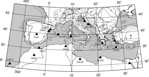
350˚ 350˚ 0˚ 0˚ 10˚ 10˚ 20˚ 20˚ 30˚ 30˚ 30˚ 30˚ 35˚ 35˚ 40˚ 40˚ 45˚ 45˚ PAB EBRE POBL CDLV VSL DUOK HVAR KOUM APER ITHO MARJ GHAR ABSA MELI KEG MDT MAHO <15 <15 20 20 20 20 20 <20 <20 25 25 25 25 25 25 <25 <25 <25 30 30 30 >30 <30 <30 30 30 30 >35 35 35 35 35 35 >35 40 40 >40 40 40 45
Figure 1. Location of the broad-band stations used in this study. The contour lines are after the Moho map of Meissner et al. (1987).
function (RF) studies are sparse in the Mediterranean area. A com-prehensive study on a Mediterranean scale has never been per-formed. Local studies have been done by Sandvol et al. (1998) who studied the stations PAB and TOL in central Spain and three sta-tions in the eastern Mediterranean (Egypt, Turkey, Israel), Paulssen & Visser (1993), who studied RF for a temporary network in Spain and Julia et al. (1998), who studied the short-period station POB in the northwest of Spain. Megna et al. (1995) performed a RF study at the Mednet station VSL on Sardinia whereas Megna & Morelli (1994) studied a Mednet station in the central Apennines. A RF study for three stations in the southern French Alps has been done by Bertrand & Deschamps (2000). In the eastern Mediterranean re-gion RF studies are even more sparse. C¸ akir et al. (2000) determined the Moho depth and crustal structure of the station TBZ in north-eastern Turkey. In Greece two detailed RF studies for visualizing the subducting slab are done by Li et al. (2001) and Knapmeyer & Harjes (2000).
Here, we present new results of RF analysis for crustal structure and thickness beneath 12 new broad-band stations and 5 known broad-band stations in the Mediterranean region including northern Africa (Fig. 1). We apply the RF technique of Ammon (1991) to teleseismic broad-band seismograms recorded by recent, temporary, seismological stations installed as part of the Mantle Investigation of the Deep Suture between Europe and Africa (MIDSEA) project (Van der Lee et al. 2001) and several permanent seismological stations in the Mediterranean (Fig. 1). To minimize and visualize the trade-off between the crustal thickness and the average Poisson’s ratio of the crust we use waveform fits of synthetic receiver functions to observed receiver functions that include phases converted at the base of the crust as well as phases that bounced within the crustal column.
2 M E T H O D
In order to solve the receiver function inverse problem we developed a grid search method with which we are able to identify Moho depth and other crustal discontinuities. We perform a complete search through a 2-D parameter space searching for the minimum misfit between the calculated synthetic RF and the observed RF. We find that sedimentary layers can play an important role in RF analysis.
2.1 Receiver functions
Teleseismic P waveforms recorded at a three-component seismic broad-band station are effective for the investigation of local crustal structure beneath the seismic station. If all effects other than the local structure beneath the receiver can be eliminated (source and propagation effects and instrument response), detailed modelling of the first 20–30 s of the waveform provides us with the structure of the crust beneath the station. For a detailed reviews/descriptions of the RF analysis/modelling technique, see Langston (1979), Owens et al. (1984) and Ammon et al. (1990). Here, we use the RF application of Ammon (1991).
We use seismograms from teleseismic events located between 30◦ and 95◦ epicentral distance and with magnitudes over 5.8. A receiver function is constructed from each seismogram by decon-volving the vertical component, which is the best estimate of plane
P-wave energy impinging on the base of the crust, from the radial
and transverse components. The resulting RF represents S-wave energy generated by discontinuous crustal structure. We selected the RF’s on low pre-signal noise and the occurrence of excessive amplitude on the radial component and the shape of the vertical component. To increase the signal-to-noise ratio we stack the set of receiver functions for each station, providing a stacked receiver function which represents the azimuthally averaged structure of the crust beneath the station. The averaging radius of the conversion points to a Moho at a depth of 30 km is around 6 km for the di-rect conversion and 22 km for the reverberated phases. Information about dipping structures and anisotropy under the stations can be obtained from azimuth-dependent RF. Unfortunately, temporary and intermittent station operation periods, limits on data quality and in-homogeneous event distribution for the stations studied prevented us from obtaining significant results on possible Moho dips and on anisotropy.
A time window is used with a total length of 70 s, starting 20 s before P to 50 s after. This time window contains Moho generated
PpPs and PpSs+PsPs, as well as similar phases from intracrustal
discontinuities. The differences between slownesses of these crustal phases with respect to the slowness of the direct P-wave are negligi-ble over the selected range of epicentral distances. Hence we stack the receiver functions for each station without move-out correction.
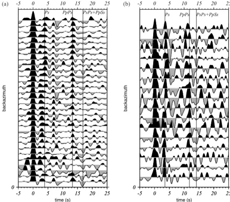
0 -5 0 5 10 15 20 25 -5 0 5 10 15 20 25 Ps PpPs PsPs+PpSs 0 backazimuth -5 0 5 10 15 20 25 time (s) 0 -5 0 5 10 15 20 25 -5 0 5 10 15 20 25 Ps PpPs PsPs+PpSs 0 backazimuth -5 0 5 10 15 20 25 time (s) (a) (b)
Figure 2. Receiver functions for two stations, PAB (a) and KOUM (b). Direct Moho conversion and reverberated phases are indicated by the vertical lines.
To stabilize the deconvolution we have evaluated the effect of so-called ‘water levels’, c, between .0001 and .1. This means that spectral holes in the frequency domain are filled up to amplitudes from .01 to 10 per cent of the maximum amplitude. We also tested different Gaussian-shaped low-pass filter cutoffs, a, between 0.5 and 1.5 Hz. We found the values c= .001 or c = .0001 and a = 2 (≈1 Hz) to yield the most stable results for 14 of the 17 stations studied here. Examples of the obtained RF’s are shown in Fig. 2 for stations PAB and KOUM. Clearly visible are the direct P-to-S converted phase and the reverberated phases PpSs+PsPs. The temporary character of the MIDSEA stations is reflected in the RF for KOUM. The RF are more noisy than the RF obtained for the permanent GSN station PAB.
2.2 Strong velocity contrast close to the surface
For some stations the arrival time of the first peak on the radial component of the RF is delayed with respect to the vertical com-ponent. This was already recognized in earlier work (e.g. Paulssen
et al. 1993; Owens & Crosson 1988) and tentatively explained by
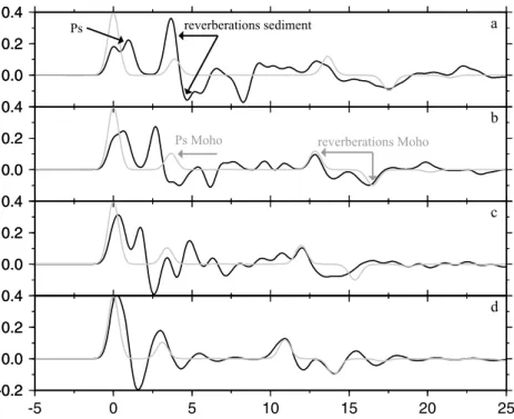
interference of the direct P-arrival with a P-to-S conversion from the base of a low velocity layer. Synthetic modelling shows that an apparent shift of the first peak of up to half of a second can be due to a strong low velocity contrast close to the surface (Fig. 3). For a thickness of 4 km for the uppermost layer the direct P and the P-to-S converted phase can be distinguished. Due to the low-velocity layer the ray turns to sub-vertical and therefore the horizontal compo-nent of the P-wave diminishes. The expected first peak is thus very small while the second peak, representing the conversion from the low-velocity layer, has larger amplitudes, resulting in an apparent delay of the first peak as compared to the vertical component. For thinner sedimentary layers interference of the peaks of the direct P
and the P-to-S conversion produces one composite peak which is shifted in time compared to the P-peak. Depending on the values for RF parameters a and c the peak can apparently shift as much as 0.5 s. Estimation of Moho depth is more difficult when sediment layers are present as the direct P-to-S conversion from the Moho can be masked by the high amplitudes of the reverberations of the sediment layer. In the synthetic tests of Fig. 3 the P-to-S conversions from the Moho are theoretically located around 3 s (Fig. 3d) to 3.5 s (Fig. 3a) but are hard to identify in the black curves as visible in some of the tests. In such cases identification of the Moho will be largely based on the coherence between the direct converted phase and phases that reverberated within the crust.
2.3 Grid search for Moho depth
We use a waveform misfit gridding method to estimate Moho depth and the associated uncertainties (Fig. 4). Waveform misfits are de-fined through the rms misfit between the observed RF and synthetic RF for different crustal model parameters. The misfit indicates how different a synthetic RF is from the observed RF. Our method is slightly different from the method of Zhu & Kanamori (2000), who evaluated the uncertainties in, and the trade-off between Moho depth and the average Poisson’s ratio of the crust, based on the combined amplitudes of the RF at predicted arrival times for the direct Ps and the multiple converted phases PpPs and PpSs+PsPs. The synthetic receiver functions in our method and the traveltime predictions in the method of Zhu & Kanamori (2000) are both based on modelling using a fixed value for the average P-wave velocity of the crust and varying Moho depth and Poisson’s ratio. The main difference be-tween our and their method is that, in addition to the timing, the amplitudes and shapes of the relevant phases are taken into account. Because we also include the direct P-arrival in the synthetic we can,
0.0 0.2 0.4 0.0 0.2 0.4 a Ps reverberations sediment 0.0 0.2 0.4 0.0 0.2 0.4 b
Ps Moho reverberations Moho
0.0 0.2 0.4 0.0 0.2 0.4 c -0.2 0.0 0.2 0.4 -5 0 5 10 15 20 25 -0.2 0.0 0.2 0.4 d
Figure 3. Synthetic examples of a shift of the first peak due to a velocity contrast close to the surface (black lines). We used a simple three layer model with
a sedimentary layer varying in thickness between (a) 4 km, (b) 3 km, (c) 2 km and (d) 1 km with a strong contrast of 3.0 km s−1at the bottom of the layer. The direct P-to-S conversion and the reverberations of the sedimentary layer (a) and Moho (b) are indicated. The Moho is located 25 km under this strong discontinuity (same in all frames). The grey lines represent the synthetic RF if no sedimentary contrast was present. In (c) and (d) an apparent shift in the direct P arrival is the result of interference with the P-to-S conversion from the base of the sedimentary layer (black line). In the presence of sedimentary layers a P-to-S conversion from the Moho can be obscured by reverberations within the sedimentary layer.
besides intra-crustal discontinuities, also model sedimentary layers (Fig. 4). Conversions from the latter can interfere with the radial component of the direct P-wave producing an apparent P-arrival on the radial component that is time-shifted with respect to the verti-cal component. Reverberations from such layers can, however, also cause low misfit levels related to apparent intracrustal discontinu-ities down to 10 km, depending on the thickness of the sedimentary layer.
By using a fixed Vp representative of the average crustal values, the velocities for the upper-crust are overestimated. The depth es-timate for a mid-crustal discontinuity at 15 km depth, indicated by the minimum misfit contour, can be off by 2 km for a difference between our average Vp for the crust and the real Vp of 1 km s−1. For a sedimentary layer 2 km thick the depth estimate can be wrong by 1.5 km for a difference of 2.5 km s−1 between our average Vp for the crust and the real Vp.
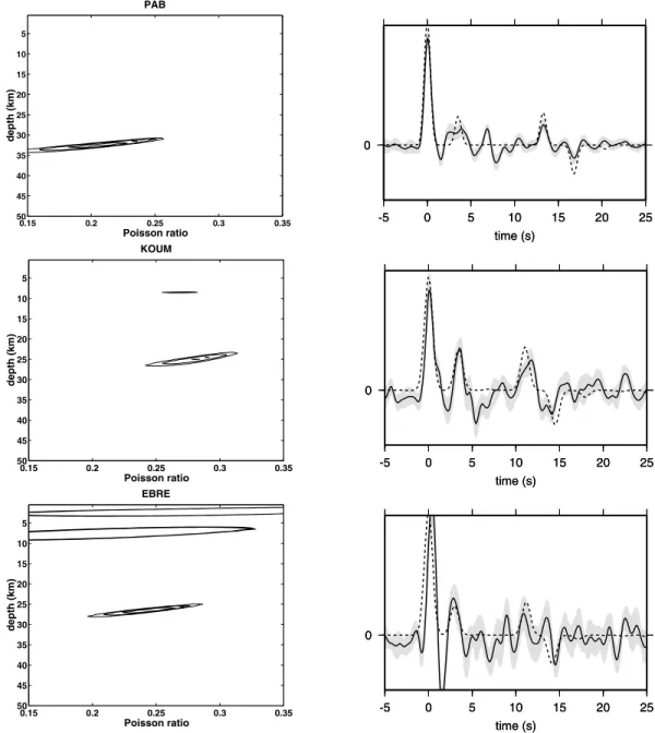
We estimate the uncertainty in the Moho depth from the shape of the misfit plot and the double standard deviation (95 per cent confi-dence interval) of the stacked RF. We estimate the error in the Moho depth and Poisson’s ratio by a 10 per cent increase in the misfit. Such an increase in misfit between model and stacked RF generally re-mains within the bounds of the double standard deviation. The error estimate for the Moho depth is practically independent of Poisson’s ratio, though the estimate of the mean Moho depth does depend on Poisson’s ratio (Fig. 4). Because errors are estimated for a specific Moho depth and Poisson’s ratio, the trade-off between depth and Poisson’s ratio is not taken into account in the scalar error estimates in Table 1.
To validate our application of the RF method we compare our results for GSN station PAB in San Pablo, Spain, with previous re-sults from the geophysical literature. Station PAB is located on the Iberian Massif. The Iberian Peninsula is a relatively stable
conti-nental region where the last major tectonic activity was in the early Oligocene (Dercourt et al. 1986; Dewey et al. 1989). We selected a set of seismograms with a high signal-to-noise (S/N) ratio from 36 events that occurred over a time period of 3 yr, and then applied the methodology just subscribed (Figs 4a and b).
In Fig. 4(a) the Moho is visible at a depth of 32 ± 0.9 km with an average Poisson’s ratio of 0.21 and an average Vp = 6.25 km s−1 for the crust. To obtain an indication of the preci-sion of this method the synthetic receiver function for the min-imum misfit model is compared with the stacked receiver func-tion (Fig. 4b). The direct Ps conversion from the Moho, at 4 s, and the reverberations, at 13 and 16.5 s are very clear (solid line). The same conversions in the synthetic receiver function (dashed line) correspond very well with the conversions in the stacked re-ceiver function. Both the direct Ps conversion and the reverbera-tions are modelled providing a well constrained estimate for Moho depth. Results for PAB agree well with the literature as discussed in Section 3.
Two other examples are shown for KOUM (Figs 4c and d) and EBRE (Figs 4e and f). The Moho is located at a depth of 25 ± 1.4 km for KOUM and 26± 1.4 km for EBRE. For both stations the synthetic RF corresponding to the minimum misfit model fits the observed RF well. The fit for the direct Ps converted phase from the Moho is satisfactory and the reverberations correspond reason-ably well. For both stations we see an indication of an additional layer in the upper crust. For KOUM we see an indication of a mid-crustal discontinuity around 8 km depth (Fig. 4c). This is also visible in the RF (Fig. 4d) where the broadening of the first peak after 1–1.5 s is caused by the direct P-to-S conversion of the mid-crustal dis-continuity. An additional contrast close to the surface is visible in the misfit plot for EBRE (Fig. 4e). In the minimum misfit (Fig. 4e) plot the contrast is visible as low misfit contours in the first 5 km. In
Poisson ratio depth (km) PAB 0.15 0.2 0.25 0.3 0.35 5 10 15 20 25 30 35 40 45 50 0 -5 0 5 10 15 20 25 time (s) 0 -5 0 5 10 15 20 25 time (s) Poisson ratio depth (km) KOUM 0.15 0.2 0.25 0.3 0.35 5 10 15 20 25 30 35 40 45 50 0 -5 0 5 10 15 20 25 time (s) 0 -5 0 5 10 15 20 25 time (s) Poisson ratio depth (km) EBRE 0.15 0.2 0.25 0.3 0.35 5 10 15 20 25 30 35 40 45 50 0 -5 0 5 10 15 20 25 time (s) 0 -5 0 5 10 15 20 25 time (s)
Figure 4. Moho thickness for three stations. Left panels (a, c, e) show the results for the grid search method for stations PAB, KOUM and EBRE. The right
panels (b, d, f) show the data RF (solid black line), the corresponding double standard deviation (grey shading) and the synthetic RF (dashed line) calculated from the one-layer model corresponding to the minimum misfit model. See the text for interpretation of the contour lines.
the RF (Fig. 4f) one can recognize the existence of a contrast close to the surface in the apparent shift of the first peak.
2.4 Crustal structure
We use the information on depth of the Moho, intracrustal disconti-nuities and sedimentary layers provided by our grid search method to construct simple initial models for layered crustal structure, ad-ditional discontinuities were added if remaining peaks in the RF in-dicated additional P-to-S converted phases. These models are then optimized by a combined process of RF inversions (using Ammon’s inversion scheme) and trial and error so that they provide the best fit to the observed receiver functions. In all cases we obtained 2-or 3-layer models with a velocity contrast near the surface and/2-or a mid-crustal discontinuity using constant seismic properties for
each layer. We report on the results of our modelling in the next section.
3 R E S U L T S A N D D I S C U S S I O N
Our best estimates for Moho depths obtained from RF analysis with the grid search method are summarized in Fig. 5 and Table 1. The values we found range from around 20 km for intra-oceanic islands and extended continental margins to near 45 km in regions where Eurasian and African continents have collided. Poisson’s ratios vary between 0.21 and 0.31 (Vp/Vs = 1.65–1.90). The average Poisson’s ratio for the 17 investigated locations is 0.26 ± 0.03 (Vp/Vs = 1.76± 0.07). We found sedimentary layers for 11 stations (Fig. 6). For 10 stations we found mid-crustal discontinuities and under 5
Table 1. Locations of broad-band stations, number of RF used and resulting
values for Moho depth, error estimate and crustal structure.
Station Latitude Longitude N Moho Error Poisson’s Error (km) (km) ratio PAB 39.546 −4.348 36 32 0.9 .21 .02 EBRE 40.823 0.494 11 26 1.4 .26 .03 POBL 41.380 1.080 17 28 1.1 .28 .02 MAHO 39.896 4.267 4 25 1.3 .24 .03 VSL 39.496 9.378 45 29 1.1 .22 .03 HVAR 43.178 16.449 30 47 1.6 .24 .02 DUOK 44.113 14.932 53 41 1.6 .28 .02 ITHO 37.179 21.925 16 43 1.7 .30 .03 KOUM 37.704 26.838 16 25 1.4 .28 .03 APER 35.550 27.174 14 29 2.3 .26 .07 CDLV 29.163 −13.444 21 19 1.5 .31 .04 MDT 32.817 −4.614 18 39 1.4 .23 .02 MELI 35.523 −2.939 52 22 1.9 .29 .04 ABSA 36.277 7.473 33 27 1.4 .28 .03 GHAR 32.122 13.089 14 30 2.1 .29 .04 MARJ 32.523 20.878 14 31 1.5 .21 .04 KEG 29.927 31.829 69 32 1.1 .25 .03
stations both a sediment layer and a mid-crustal discontinuity were found. For CDLV we found two mid-crustal discontinuities and a weak velocity contrast at the Moho. We used for all stations an av-erage crustal velocity of Vp= 6.25 km s−1except for three stations (DUOK, HVAR and CDLV) where literature suggested lower aver-age crustal velocities and we used Vp= 6.0 km s−1. We assume a sharp Moho discontinuity in the waveform modelling. In reality the Moho velocity contrast could take place over an interval of finite width. However, this interval is at most 2 km wide while for most of the stations it was even less than 1 km. For wider intervals the peaks of the converted phases were too broad to fit the RF. In the inversion of the RF we allowed the upper-mantle velocity to vary. This resulted in lower average upper-mantle velocities under the in-vestigated stations than the reference Vp= 8.0 km s−1from IASP91 (Kennett & Engdahl 1991). For 11 stations we found upper-mantle velocities lower than IASP91, 5 stations had upper mantle velocities equal to IASP91 and 1 station was faster. Upper-mantle velocities vary between Vp= 7.6 km s−1under MELI and Vp= 8.2 km s−1
un-350˚ 350˚ 0˚ 0˚ 10˚ 10˚ 20˚ 20˚ 30˚ 30˚ 30˚ 30˚ 35˚ 35˚ 40˚ 40˚ 45˚ 45˚
32
±0.9
26
±1.4 28±1.1
19
±1.5
29
±1.1
41
±1.6
47
±1.6
25
±1.4
29
±2.3
43
±1.7
31
±1.5
30
±2.1
27
±1.6
22
±1.9
32
±1.1
39
±1.4
25
±1.3
PAB EBRE POBL CDLV VSL DUOK HVAR KOUM APER ITHO MARJ GHAR ABSA MELI KEG MDT MAHOFigure 5. Result of the waveform misfit gridding method for crustal thickness under the stations.
der APER. However, it is possible that mantle velocities are slightly underestimated by the inversion scheme. Because the amplitudes of the synthetic RF are for most stations higher than the real amplitudes in the data (because we use no more than three crustal discontinu-ities), the inversion tries to correct for this difference in amplitude by decreasing the velocity jump at the discontinuity. The average velocity jump at the Moho was between Vp= 1.2 km s−1and Vp= 1.7 km s−1.
We will discuss the results for all stations in the following sec-tions. Stations are ordered and grouped depending on geographical location and availability of references.
3.1 PAB
The depth we found for the Moho below PAB, 32± .9 km, is con-sistent with depth estimates in previous studies. In central Spain there have been several refraction and deep seismic sounding pro-files which located the Moho in this region at 31 km depth (Banda
et al. 1981b), 31 km by Surinach & Vegas (1988) and 34 km found
by the ILIHA DSS GROUP (1993). Other receiver function analysis is done by Sandvol et al. (1998), who found a deeper Moho of 34 km for the same station, and Paulssen & Visser (1993) who found a thinner crust of 29 km for this area. Paulssen & Visser (1993) also used a lower average P-velocity of 6 km s−1. A Moho at 29 km and a
Vp= 6 km s−1does also fit the observed Ps from the Moho, but does not fit the corresponding reverberated phases, which have not been taken into account by Paulssen & Visser (1993). The result of Sand-vol et al. (1998) agrees with our estimate within the error bounds. The peak just before the P-to-S converted phase of the Moho is probably a converted phase from a mid-crustal discontinuity. Our depth of 20 km for this discontinuity is in agreement with Sandvol
et al. (1998). The refraction profiles of Banda et al. (1981b) and
Surinach & Vegas (1988) located a discontinuity slightly deeper around 23–24 km. This discontinuity is not visible in the waveform misfit plot (Fig. 4a) because the peaks of the direct converted phase and the reverberation do not correspond very well. Therefore the misfit for this discontinuity is relatively high with respect to the misfit we found for the Moho and we do not see it in the waveform misfit plot. If we chose different misfit contour lines the discontinu-ity could be made visible.
-5 0 5 10 15 20 25 time (s) 0 10 20 30 40 50 depth (km) 2 4 6 8 v (km s-1) PAB -5 0 5 10 15 20 25 time (s) 0 10 20 30 40 50 depth (km) 2 4 6 8 v (km s-1) EBRE -5 0 5 10 15 20 25 time (s) 0 10 20 30 40 50 depth (km) 2 4 6 8 v (km s-1) POBL -5 0 5 10 15 20 25 time (s) 0 10 20 30 40 50 depth (km) 2 4 6 8 v (km s-1) MAHO -5 0 5 10 15 20 25 time (s) 0 10 20 30 40 50 depth (km) 2 4 6 8 v (km s-1) VSL -5 0 5 10 15 20 25 time (s) 0 10 20 30 40 50 depth (km) 2 4 6 8 v (km s-1) HVAR -5 0 5 10 15 20 25 time (s) 0 10 20 30 40 50 depth (km) 2 4 6 8 v (km s-1) DUOK -5 0 5 10 15 20 25 time (s) 0 10 20 30 40 50 depth (km) 2 4 6 8 v (km s-1) ITHO -5 0 5 10 15 20 25 time (s) 0 10 20 30 40 50 depth (km) 2 4 6 8 v (km s-1) KOUM -5 0 5 10 15 20 25 time (s) 0 10 20 30 40 50 depth (km) 2 4 6 8 v (km s-1) APER
Figure 6. Modelling of the RF for the crustal structure beneath the stations. For every station the best fitting model containing not more than 3 layers is shown
in the left frame (data in solid lines, synthetic in dashed lines, double standard deviation on the data in grey). The corresponding model in the right frame shows the P- (dotted line) and S-velocities (dashed line).
-5 0 5 10 15 20 25 time (s) 0 10 20 30 40 50 depth (km) 2 4 6 8 v (km s-1) CDLV -5 0 5 10 15 20 25 time (s) 0 10 20 30 40 50 depth (km) 2 4 6 8 v (km s-1) MDT -5 0 5 10 15 20 25 time (s) 0 10 20 30 40 50 depth (km) 2 4 6 8 v (km s-1) MELI -5 0 5 10 15 20 25 time (s) 0 10 20 30 40 50 depth (km) 2 4 6 8 v (km s-1) ABSA -5 0 5 10 15 20 25 time (s) 0 10 20 30 40 50 depth (km) 2 4 6 8 v (km s-1) GHAR -5 0 5 10 15 20 25 time (s) 0 10 20 30 40 50 depth (km) 2 4 6 8 v (km s-1) MARJ -5 0 5 10 15 20 25 time (s) 0 10 20 30 40 50 depth (km) 2 4 6 8 v (km s-1) KEG Figure 6. (Continued.)
3.2 EBRE, POBL, MAHO
The neighbouring stations POBL and EBRE show the Moho at 28 ± 1.1 km and 26 ± 1.4 km depth (Fig. 6), respectively, which is in agreement with the 29–31 km for POBL and the 26–28 km for EBRE found by Gallart et al. (1995) and Zeyen et al. (1985). But our values are slightly shallower than the 30 km from Meissner et al. (1987), which is based on interpolation, and the 32 km from a re-ceiver function study of the short-period station POB (Julia et al. 1998). Julia et al. (1998) found four different models fitting the re-ceiver function ranging from 29 to 38 km Moho depth. The timing of our direct P-to-S converted phase and theirs is approximately equal, both around 3.7 s. Differences occur in the interpretation of the
re-verberated phases. We base our interpretation of the reverberations on the strong correlation between the direct phase and the reverber-ated phases for a specific Poisson’s ratio. This results in reverberreverber-ated phases at approximately 11.5 s and 15 s Julia et al. (1998) interpret phases at 14 and 18 s as reverberations from the Moho.
For MAHO (Hanka & Kind 1994), located on Menorca, we found 25± 1.3 km for the crustal thickness (Fig. 6). This values agrees very well with results from seismic profiles from Gallart et al. (1995) and Collier et al. (1994). They found crustal thicknesses of around 23– 25 km for Mallorca and between Mallorca and Menorca. Although we only used four events we found a clear indication of the Moho. More detailed modelling of the upper-crustal structure showed an additional discontinuity at 5 km depth.
3.3 VSL
For VSL (Boschi et al. 1991) we find the Moho at 29± 1.1 km (Fig. 6), using the grid search method. This station has been previ-ously studied by Megna et al. (1995). Our result of 29 km is in very good agreement with their observation of 29–30 km and also with the 28 km from refraction profiles from Egger (1992) for the same region. More detailed modelling (Fig. 6) shows discrepancies. We find a sedimentary layer but do not need a mid-crustal discontinu-ity to fit the RF. In contrast, Megna et al. (1995) find a mid-crustal discontinuity at a varying depth of 21–25 km and do not include a sedimentary layer. Upper-mantle P-velocities are the same in both studies at 7.8 km s−1. From the refraction profiles Egger (1992) finds a small velocity contrast around 18 km depth but also finds a strong velocity contrast close to the surface.
3.4 HVAR, DUOK
Along the coast in Croatia a crustal thickness of 47± 1.6 km with a Poisson’s ratio of 0.24 is found for HVAR (Fig. 6). This is signif-icantly deeper than the approximately 35 to 42 km thickness found in the refraction profiles of Dragaˇsevi´c & Andri´c (1968), the later Moho maps from Meissner et al. (1987) and the local Moho maps from Aljinovi´c (1987) and Morelli (1998). We used a relatively low average velocity P velocity of 6.0 km s−1for the crust to account for the thick sediment layers in this region. Aljinovi´c (1983) and Morelli (1998) suggested sediment layers in the Adriatic region ranging in thickness between 8 and 15 km. If we assume a higher Poisson’s ra-tio for the crustal average, then thinner crust is obtained (e.g. 43 km for a Poisson’s ratio of 0.30) but this model is 10 per cent less ca-pable of simultaneously fitting the direct P-to-S conversion and the reverberations. If we allow one more layer we obtain the best fit with a thin, low velocity layer at the surface and an 11 km thick under-lying sedimentary layer (Fig. 6). With these two layers most of the peaks in the RF can be fit well. Modelling with thinner crust leads to unsatisfying fits between the data and the synthetic. However, if the sedimentary layer is stripped off, the crustal thickness under HVAR compares well to standard continental crustal thickness. For DUOK we found a comparable thick sedimentary layer of 10 km (Fig. 6). The Moho depth of 41± 1.6 km is in reasonable agreement with previous studies in the region although our depth estimate is slightly larger than suggested by these studies (Dragaˇsevi´c & Andri´c 1968; Meissner et al. 1987; Aljinovi´c 1987; Morelli 1998).
3.5 ITHO, KOUM, APER
For the station ITHO we found a crustal thickness of 43± 1.7 km (Fig. 6) which is consistent with the Moho map of Ansorge et al. (1992). But Makris (1985) and Meissner et al. (1987) found values closer to 35 km. The source of this large difference in Moho depth is unclear. The maps from Meissner et al. (1987), Ansorge et al. (1992) and Makris (1985) are interpolated maps where it is often difficult to locate the base values for interpolation. This holds also for station ITHO which is at the borders of the map of Ansorge
et al. (1992) which are susceptible to extrapolation errors. Also for
the other maps it is unclear if the Moho depth for this area is based on individual data points or interpolation between data points.
Also for KOUM we found a large discrepancy between our 25± 1.4 km (Fig. 6) and the 32 km found by Makris (1985) and Meissner
et al. (1987). Because both KOUM and APER are located outside
the bounds of the map of Ansorge et al. (1992) no comparison is possible. The island Samos is at the borders of the maps of Makris
(1985) and Meissner et al. (1987) so the differences of the results for this area are probably due to edge effects in the maps. The Moho is very clear in the waveform misfit plot and the RF (Fig. 4c and d). The more detailed modelling shows that we obtain a reasonable fit for all peaks in the first 10–15 s if we take into account a mid-crustal discontinuity at 11 km depth. For APER, our 29± 2.3 km crustal thickness (Fig. 6) is consistent with the studies from Meissner et al. (1987) and Makris (1985).
3.6 CDLV
The station CDLV is located on the island Lanzarote, Canary Is-lands. In the waveform misfit plot we identify 3 different disconti-nuities around 5 km, 11 km and the Moho at 19± 1.5 km depth which are incorporated in the model shown in Fig. 6. These results are comparable with results from Banda et al. (1981a) who found discontinuities around 4 and 11 km depth. Below this second dis-continuity they derived a velocity of 7.4 km s−1. They did not find any indication for a deeper discontinuity, at least down to 25–30 km, which could be interpreted as the crust-mantle boundary. For the nearby island of Gran Canaria they found a mid-crustal disconti-nuity at 1–2 km depth and another discontidisconti-nuity around 13 km depth which they identified as the Moho. But their data for Gran Canaria is rather scarce. Ye et al. (1999) performed a refraction profile for Gran Canaria where they found a crustal structure which was very com-parable to the crustal structure under Lanzarote from Banda et al. (1981a). Ye et al. (1999) found discontinuities at around 4 and 11 km depth. They locate the Moho around 18–20 km depth. Approaching the island the strong reflection of the Moho becomes increasingly unclear and eventually almost disappears in the vicinity of the island. This can be due to a velocity gradient at the Moho instead of sharp discontinuity. This velocity gradient can be due to magmatic un-derplating beneath the oceanic crust (Freundt & Schmincke 1995). This was already observed for other intra-plate volcanic islands, as in Hawaii (Watts & ten Brink 1989) and the Marquesas (Caress
et al. 1995). Probably a similar phenomenon also takes place under
Lanzarote explaining the diminishing amplitudes in the refraction profiles which caused the absence of a sharp Moho. Because we use much lower frequencies we can still detect this contrast but we see in the detailed modelling (Fig. 6) that the velocity contrast at the Moho is small.
3.7 MDT, MELI, ABSA
For the three western most stations along the North African coast, MDT, MELI and ABSA, we found crustal thicknesses of 39± 1.4 km for MDT, 22± 1.9 km for MELI and 27 ± 1.4 km for ABSA (Fig. 6). Our depth of 39 km for MDT, found after stacking 18 events, is slightly deeper than the 36 km found by Sandvol et al. (1998) for the same station after stacking 4 events. However, Sandvol et al. (1998) also modelled a velocity jump at 39 km to fit the RF which they did not interpret as the Moho. This is in agreement with the geographical location of the station in the Atlas mountains where one would expect a thickened crust.
The 27 km depth found for ABSA is in agreement with refraction profiles from (Egger 1992) for the Tunisian coast. Both the values for ABSA and MELI are in reasonable agreement with crustal thick-nesses derived through analysis of gravity data (Mickus & Jallouli 1999). For ABSA we found a weak contrast close to the surface and a mid-crustal discontinuity at 12 km depth. With these two addi-tional layers we are capable of modelling every peak in the first 10 s
of the RF and the reverberations from the Moho. The 22 km Moho depth for MELI is also in agreement with 22 km crustal thickness found by Torn´e et al. (2000) after modelling of gravity, elevation and heat flow data. MELI is a very noisy station where large re-verberations with high amplitudes are visible. No clear mid-crustal discontinuity is present but we found a large contrast close to the sur-face. To decrease the influence of the noise we used every possible event recorded to average out the noise contribution. Unambiguous identification of the Moho is difficult in this case due to the large amplitudes visible in the RF. The Moho-converted phases are prob-ably overwhelmed by the reverberations from the contrast close to the surface and by the noise. It is possible that more models fit this RF which are not in agreement with the gravity model.
3.8 GHAR, MARJ, KEG
For the two Libyan stations, GHAR and MARJ, we have found Moho depths of 30± 2.1 km and 31 ± 1.5 km, respectively (Fig. 6). We found for both stations a low velocity layer at the surface with a thickness of approximately 2 km and did not need a mid-crustal discontinuity to explain the main features of the RF. For GHAR it was not possible to find one single solution with the grid search method. Because the peak, which we identify as the Moho, is very broad, the Moho depth can vary between 30 and 36 km where the misfit method indicates lowest misfits for 30 and 36 km. After in-terpretation of both possible models we decided that the 30 km solution is probably the most reliable. There was a better fit for the multiples although the errors are so large that the peaks of the multi-ples are hardly significant. For a more robust interpretation we need more data. Under the Egyptian station KEG (Boschi et al. 1991) the Moho is located at a depth of 32± 1.1 km with a Poisson’s ratio of .25. A mid-crustal discontinuity was found at a depth of 10 km (Fig. 6). The Moho depth compares well to the 33 km depth found by Sandvol et al. (1998), a RF study of nine events, and the ap-proximately 31 km depth found by Makris et al. (1988) for northern Egypt.
4 C O N C L U S I O N S
We have derived simple crustal models from stacked receiver func-tions for twelve MIDSEA and five permanent seismological stafunc-tions in the Mediterranean providing data for new locations in the Mediter-ranean region including northern Africa. Our models are simple in the sense that they contain no more than three layers with constant seismic velocities that represent layer averages. We derive Moho depth and average Poisson’s ratio of the crust from a grid search for the best fitting synthetic RF, containing both direct conversion and reverberated phases. We use the density of the misfit contours as well as the standard deviation of the stacked receiver functions to estimate the uncertainty on the derived Moho depths and average Poisson’s ratios. Our results are summarized in Table 1 and Fig. 5. We found that the Moho under the stations is a sharp discontinuity spanning less than 2 km in depth. The velocity contrast for Vp at
the Moho varies under most stations between 1.2 and 1.7 km s−1. Upper-mantle P-velocities are slightly slower than IASP91, only one station is faster than IASP91, and vary between Vp= 7.6 km s−1and Vp= 8.2 km s−1.
On comparison of our results with Moho maps inferred from inter-polated reflection and refraction data, we find that for some regions the agreement is very good, while for other regions the interpolated values deviate from our observations. The largest deviations were
found in Croatia and Greece. We also provide data on crustal struc-ture beyond the geographic bounds of existing Moho maps for the Mediterranean region.
The values we found for Moho depths range from around 20 km for intra-oceanic islands and extended continental margins to near 45 km in regions where the Eurasian and African continents have col-lided. Moho depth for a Canary Island and a Balearic island appear to be similar to Moho depths below the Moroccan and northeastern Spanish continental margins, respectively. The eastern part of the North African continental margin is relatively undisturbed by cur-rent Mediterranean tectonics and shows Moho depths of 30–32 km, which are close to a standard continental crustal thickness of 33 km. The crust of this passive margin is 5 to 10 km thicker than that of the more disturbed western part of the North African continen-tal margin. The Hellenides, located above subducting lithosphere, show large variations in crustal thickness, from 42 km in the west to 29 km in the east. The extremely thick crust of the eastern Adriatic margin compares well to standard continental crustal thickness after the thick sedimentary layers are stripped off.
A C K N O W L E D G M E N T S
We are grateful to J. Ansorge and F. Marone for insigthful comments and pointers to previous works. We appreciate comments from an anonymous reviewer, which improved the manuscript. Funding for this study was provided by the Swiss National Science Foundation (SNF). Financial support for MIDSEA came from the SNF, with additional support from the Carnegie Institution of Washington, the French National Scientific Research Center and the University of Nice at Sophia-Antipolis, the Italian National Institute of Geo-physics and Volcanology, and numerous local organizations (see Van der Lee et al. 2001). We thank the many individuals associated with MIDSEA (see Van der Lee et al. 2001); their support has been invalu-able. Data for PAB (GSN), MAHO (Geofon), and VSL, KEG and MDT (all MedNet) were obtained from the ORFEUS Data Center, the GEOFON Data Center, and the IRIS DMC, respectively. Con-tribution number 1262 of the Institute of Geophysics, ETH Zurich.
R E F E R E N C E S
Aljinovi´c, B., 1983. The deepest seismic horizons in the northeastern Adri-atic, PhD thesis, University of Zagreb, Zagreb.
Aljinovi´c, B., 1987. On certain characteristics of the Mohoroviˇci´c disconti-nuity in the region of Yugoslavia, Acta Geologica, 17, 13–20.
Ammon, C., 1991. The isolation of receiver effects from teleseismic P wave-forms, Bull. seism. Soc. Am., 81, 2504–2510.
Ammon, C., Randall, G. & Zandt, G., 1990. On the non-uniqueness of receiver function inversions, J. geophys. Res., 95, 15 303–15 318. Ansorge, J., Blundell, D. & Mueller, S., 1992. Europe’s lithosphere-seismic
structure, in A Continent Revealed: the European Geotraverse, eds Blundell, D., Freeman, R. & Mueller, S., Cambridge University Press, Cambridge.
Banda, E., Da˜nobeitia, J., Surinach, E. & Ansorge, J., 1981a. Features of crustal structure under the Canary Islands, Earth planet. Sci. Lett., 55, 11–24.
Banda, E., Surinach, E., Aparicio, A., Sierra, J. & de la Parte, E.R., 1981b. Crust and upper mantle structure of the central Iberian Meseta (Spain), Geophys. J. R. astr. Soc., 67, 779–189.
Bertrand, E. & Deschamps, A., 2000. Lithospheric structure of the southern French Alps inferred from broadband analysis, Phys. Earth planet. Inter.,
122, 79–102.
Boschi, E., Giardini, D. & Morelli, A., 1991. MedNet: the very broad-band seismic network for the Mediterranean, Il Nuovo Cimento, 14, 79–99.
C¸ akir, ¨O., Erduran, M., C¸ inar, H. & Yilmazt¨urk, A., 2000. Forward modelling receiver functions for crustal structure beneath station TBZ (Trabzon, Turkey), Geophys. J. Int., 140, 341–356.
Caress, D., McNutt, M., Detrick, R. & Mutter, J., 1995. Seismic imaging of hotspot related crustal underplating beneath the Marquesas islands, Nature, 373, 600–603.
Collier, J., Buhl, P., Torn´e, M. & Watts, A., 1994. Moho and lower crustal reflectivity beneath a young rift basin: results from a two-ship, wide-aperture seismic-reflection experiment in the Valencia Through (western Mediterranean), Geophys. J. Int., 118, 159–180.
Dercourt, J. et al., 1986. Geological evolution of the Tethys Belt from the Atlantic to the Pamirs since the Lias, Tectonophysics, 123, 241–315. Dewey, J., Helman, M., Turco, E., Hutton, D. & Knott, S., 1989. Kinematics
of the western Mediterranean, in Alpine tectonics, Special Publication 45, pp. 265–283, eds Coward, M., Dietrich, D. & Park, R., Geological Society, London.
Dragaˇsevi´c, T. & Andri´c, B., 1968. Deep seismic soundings of the Earth’s crust in the area of the Dinarides and the Adriatic Sea, Geophys. Prospect.,
16, 54–76.
Egger, A., 1992. Lithosperic structure along a transect from the northern Apennines to Tunisia derived from seismic refraction data, PhD thesis, ETH Zurich, Zurich.
Freundt, A. & Schmincke, H.-U., 1995. Petrogenesis of rhyolite-trachyte-basalt composite ignimbrite P1, Gran Canaria, Canary Islands, J. geophys. Res., 100, 455–474.
Gallart, J., Vidal, N. & Da˜nobeitia, J., 1995. Multichannel seismic image of the crustal thinning at the NE Iberian margin combining normal and wide angle reflection data, Geophys. Res. Lett., 22, 489–492.
Hanka, W. & Kind, R., 1994. The GEOFON Program, IRIS Newsletter, 13, 1–4.
ILIHA DSS GROUP, 1993. A deep seismic sounding investigation on litho-spheric heterogeneity and anisotropy in Iberia, Tectonophysics, 221, 35– 51.
Jonge, M.D., Wortel, M. & Spakman, W., 1994. Regional scale tectonic evolution and the seismic velocity structure of the lithosphere and upper mantle: The Mediterranean region, J. geophys. Res., 99, 12 091–12 108. Julia, J., Vila, J. & Macia, R., 1998. The receiver structure beneath the Ebro
basin, Iberian peninsula, Bull. seism. Soc. Am., 88, 1538–1547. Kennett, B. & Engdahl, E., 1991. Traveltimes for global earthquake location
and phase identification, Geophys. J. Int., 105, 429–465.
Knapmeyer, M. & Harjes, H.-P., 2000. Imaging crustal discontinuities and the downgoing slab beneath western Crete, Geophys. J. Int., 143, 1–21. Langston, C., 1979. Structure under Mount Rainier, Washington, inferred
from teleseismic body waves, J. geophys. Res., 84, 4749–4762. Li, X. et al., 2001. A receiver function study of the Hellenic subduction zone,
European Geophysical Society Newsletter, 78, 64.
Makris, J., 1985. Geophysics and geodynamic implications for the evolution of the Hellenides, in Geological Evolution of the Mediterranean Basin, pp. 231–248, eds Stanley, D. & Wezel, F., Springer, Berlin.
Makris, J., Rihm, R. & Allam, A., 1988. Some geophysical aspects of the evolution and the structure of the crust in Egypt, in The Pan-African Belt of Northeast Africa and Adjacent Area: Tectonic Evolution and Economic
Aspects of a Late Proterozoic Orogen, pp. 345–369, eds El-Gaby, S. & Geriling, R., Braunschweig, Vieweg, Wiesbaden, Germany.
Megna, A. & Morelli, A., 1994. Determination of Moho depth and dip beneath MedNet station AQU by analysis of broadband receiver functions, Annali di geofisica, XXXVII, 913–928.
Megna, A., Morelli, A., Santini, S. & Vetrano, F., 1995. Determinazione della struttura della Moho in Sardegna meridionale mediante analisi della funzione die risposta crostale della stazione MedNet VSL, 13. Convegno, Gruppo Nazionale di Geofisica della Terra Solida, pp. 117– 124.
Meissner, R., Wever, T. & Fl¨uh, E., 1987. The Moho in Europe – Implications for crustal development, Ann. Geophysicae, 5B, 357–364.
Mickus, K. & Jallouli, C., 1999. Crustal structure beneath the Tell and Atlas Mountains (Algeria and Tunisia) through the analysis of gravity data, Tectonophysics, 314, 373–385.
Mooney, W., Laske, G. & Masters, T., 1998. CRUST 5.1: a global crustal model at 5◦× 5◦, J. geophys. Res., 103, 727–747.
Morelli, C., 1998. Lithospheric structure and geodynamics of the Italian peninsula derived from geophysical data: a review, Mem. Soc. Geol. It.,
52, 113–122.
Owens, T. & Crosson, R., 1988. Shallow structure effects on broadband teleseismic P-waveforms, Bull. seism. Soc. Am., 78, 96–108.
Owens, T., Zandt, G. & Taylor, S., 1984. Seismic evidence for an ancient rift beneath the Cumberland Plateau, Tennessee: a detailed analysis of broadband teleseismic P waveforms, Bull. seism. Soc. Am., 77, 7783– 7795.
Paulssen, H. & Visser, J., 1993. The crustal structure in Iberia inferred from P-wave coda, Tectonophysics, 221, 111–123.
Paulssen, H., Visser, J. & Nolet, G., 1993. The crustal structure from tele-seismic P-wave coda; i. Method, Geophys. J. Int., 112, 15–25.
Sandvol, E., Seber, D., Calvert, A. & Barazangi, M., 1998. Grid search modelling of receiver functions: Implications for crustal structure in the Middle East and North Africa, J. geophys. Res., 103, 26 899–26 917. Surinach, E. & Vegas, R., 1988. Lateral inhomogeneities of the Hercynian
crust in central Spain, Phys. Earth planet. Inter., 51, 226–234.
Torn´e, M., Fern´andez, M., Comas, M. & Soto, J., 2000. Lithospheric structure beneath the Alboran Basin; results from 3-D gravity modeling and tectonic relevance, J. geophys. Res., 105, 3209–3228.
Van der Lee, S. et al., 2001. Eurasia-Africa Plate Boundary Region Yields New Seismographic Data, EOS, Trans. Am. geophys. Un., 82, 637–646. Watts, A. & ten Brink, U., 1989. Crustal structure, flexure and subsidence
history of the Hawaiian Islands, J. geophys. Res., 94, 10 473–10 500. Wortel, M. & Spakman, W., 2000. Subduction and slab detachment in the
Mediterranean-Carpathian region, Science, 290, 1910–1917.
Ye, S., Canales, J., Rihm, R., Da˜nobeitia, J. & Gallart, J., 1999. A crustal transect through the northern and northeastern part of the volcanic edifice of Gran Canaria, Canary Islands, Geodynamics, 28, 3–26.
Zeyen, H., Banda, E., Gallart, J. & Ansorge, J., 1985. A wide angle seismic reconnaissance survey of the crust and upper mantle in the Celtiberian Chain of eastern Spain, Earth planet. Sci. Lett., 75, 393–402.
Zhu, L. & Kanamori, H., 2000. Moho depth variation in southern California from teleseismic receiver functions, J. geophys. Res., 105, 2969–2980.