Advanced optical microscopy toolkits for non-invasive imaging in oncology

Advanced Optical Microscopy Toolkits for

Non-Invasive Imaging in Oncology

by

Sam Osseiran

B.Eng., Polytechnique Montreal (2013)

Submitted to the Harvard-MIT Program in Health Sciences and

Technology

in partial fulfillment of the requirements for the degree of

Doctor of Philosophy in Medical Engineering and Medical Physics

at the

MASSACHUSETTS INSTITUTE OF TECHNOLOGY

September 2018

Massachusetts Institute of Technology 2018. All rights reserved.

Signature redacted

A uthor ...

Harvard-MIT Program in Health Sciences and Technology

August 24, 2018

Certified by

...

Signature redacted

Conor

vans, PhD

Assistant Professor of Dermatology, Harvar Medical School,

Wellman Center for Photomedicine, Massachusetts General Hospital

"'2 T esis

Supervisor

Signature redacted

S

A ccepted by ...

...

Emery N. Brown, MD, PhD

Director, Harvard-MT Program in Health Sciences and Technology

Professor of Computational Neuroscience and Health Sciences and

MASSACHUSTS INSTITUTE _Technology

OF TECHNOLOGY

Tecnoog

OCT 092018

MITLibraries

77 Massachusetts Avenue

Cambridge, MA 02139

http://Iibraries.mit.edu/ask

DISCLAIMER NOTICE

Due to the condition of the original material, there are unavoidable flaws in this reproduction. We have made every effort possible to provide you with the best copy available.

Thank you.

The images contained in this document are of the best quality available.

Advanced Optical Microscopy Toolkits for Non-Invasive

Imaging in Oncology

by

Sam Osseiran

Submitted to the Harvard-MIT Program in Health Sciences and Technology on August 24, 2018, in partial fulfillment of the

requirements for the degree of

Doctor of Philosophy in Medical Engineering and Medical Physics

Abstract

Despite significant advances in the fields of biophotonics and oncology alike, several challenges persist in the study, assessment, and treatment of cancer, ranging from the accurate identification and examination of potential risk factors, early diagnosis of dysplastic lesions, and monitoring of the complex heterogeneity of cellular popula-tions within tumors. To study such dynamics at the microscale, non-invasive optical toolkits offer the potential to identify, characterize, and visualize key molecules and their interactions in their native biological context, ranging from in vitro cell cul-tures to in vivo studies in both animal models and humans. In the present thesis, examples of such applications of optical tools will be presented, including: (1) the assessment of cellular oxidative stress in ex vivo human skin cultures by imaging en-dogenous and exogenous fluorescent compounds using two-photon excitation fluores-cence (TPEF) and fluoresfluores-cence lifetime imaging microscopy (FLIM); (2) visualizing water and lipid distribution as well as cellular morphology using coherent Raman scattering (CRS) imaging techniques in the stratum corneum, the most superficial layer of the epidermis; (3) using photoconvertible labels to optically tag cell subpopu-lations of interest in situ for long-term monitoring of heterogeneous cell cultures from in vitro monolayers to in vivo xenograft models; (4) visualizing melanin species in the context of melanoma with coherent anti-Stokes Raman scattering (CARS) and sum-frequency absorption (SFA) microscopies. Altogether, development of such advanced microscopy toolkits will serve to improve both understanding of cancer pathology, as well as to validate clinical diagnostic and therapeutic strategies.

Thesis Supervisor: Conor L. Evans, PhD

Title: Assistant Professor of Dermatology, Harvard Medical School, Wellman Center for Photomedicine, Massachusetts General Hospital

Acknowledgments

None of the work presented in this thesis would have been possible without all the wonderful people that I have had the pleasure of calling my friends and colleagues throughout the past 5 years. First and foremost, an enormous thank you to all the members - past and present - of the Evans team. I have had the incredible privilege of working closely with a number of talented graduate students (Alex Nichols and Joachim "Api" Pruessner), postdoctoral fellows (Tracy Wang, Lauren Austin, Zongxi Li, Manolis Rousakis, Gayatri Joshi, Sinyoung Jeong, Haley Marks, Alex Fast, Amin Feizpour, John Nguyen, Juanpe Cascales-Sandoval, and others), lab technicians (Nick Nowell, Jawad Hoballah, Fatima Mubarak, Raymond Lopez, and Michael Murphy), as well as our quintessential lab admin (Alice Chao). Of course, this fantastic team was led by Conor Evans, who has taught me virtually all I know about the implementation and use and optical imaging. From the informal white board chalk talks in his office to his coaching sessions at my very first international conference (SPIE Photonics West back in January 2015), Conor has mentored me throughout all critical stages of graduate school. It is thanks to him - and, of course, the various iterations of the lab team - that I have become the well-rounded scientist I am today. Of all the learning and life experiences I will have gained throughout the 5 years spent within the Evans group however, the daily banter, general camaraderie, and truly awesome work atmosphere within the team is certainly what I will remember and cherish most of all.

On the topic of mentorship, I would also like to extend my thanks to Dr. Jagesh Shah, who has served as my thesis committee chair, as well as Dr. Gabriela Schlau-Cohen, who agreed to take the role of thesis reader. Their considerable advice and guidance have helped navigate my scientific curiosity throughout the final years of graduate school, in addition to helping shape this thesis into the complete body of work that it is.

Next, I owe many thanks to my roommates over the past few years: Chris Lee, Benny Maimon, Fernando Martinez, and Gio Sturla. Each one of you have

con-tributed in your own ways to making life on Saint Paul Street the adventure that it was. Additional thanks go out to Taylor Gill and Colin Buss, without whom Thurs-day nights would not have been the same. Another particular round of thanks go out to my dearest friends Emily Lindemer and Liam Loscalzo, who have been my family away from home for my entire time in Boston. From the evenings spent hanging at the apartment with Zoom to the many trivia nights at Charlie's we've so joyously lost, my life in Boston would not at all have been the same without you.

I would also like to thank all my friends from back home in Montreal who have

taken the time to come down to visit me in Boston throughout the years. I warmly extend acknowledgements to Max Lefevre, Phil Cazelais, Marc-Antoine Dumoulin, and Francis Hamel (RIP); Andreanne Goyette, Steph Andrieux, Ariane Couture, and Amelie Duval Courchesne; Max Milanovic, Laura Glenn, Simran Dewan, Evan Weber, and Max Bellefeuille; Vincent Boul6" and Charlotte Girod; Stephanie Bernard and Sarah Power; and all others who have kindly stopped by to send their regards while in town. It certainly would have been a long 5 years without the continuous visits from my dearest friends from my hometown.

Additionally, I would like to express a warm thanks to all the members of my family who have supported me throughout my graduate school path. Foremost, I thank my parents Bita Danechi and Amir Osseiran for their unwavering support every step of the way; my sister Lina Osseiran, as well as my brother-in-law Quentin Dutilleul and my nephew Felix Dutilleul; my aunt Hana Osseiran; and all other family members who have been so warm and welcoming during each and every single one of my return trips home.

Finally, I would like to express my greatest thanks to my fiancee Alexandra Pee-bles. We had initially met when I was less than halfway through graduate school, back in December 2015, and endured the vast majority of our relationship apart. Nevertheless, she has been my source of comfort and peace since the day we started dating, supporting me through the most stressful aspects of graduate life. Whether it was anxiety related to meeting deadlines or rehearsing for upcoming presentations, she would offer rational advice and guidance to help me navigate through my most

difficult moments. Alexandra, thank you for your unfaltering love and support, and

simply for making my life what it now is - I cannot wait to see what our future has

Contents

1 Theory and Principles of Nonlinear Optics for Biomedical Imaging 29 1.1 Introduction . . . .

1.2 Two-Photon Excitation Fluorescence (TPEF) . . . . 1.3 Fluorescence Lifetime Imaging Microscopy (FLIM) . . . .

1.3.1 Time-Correlated Single Photon Counting (TCSPC)

1.3.2 Time-Domain Analysis . . . .

1.3.3 Phasor Analysis . . . .

1.4 Ram an Scattering . . . . 1.4.1 Spontaneous Raman Scattering . . . .

1.4.2 Coherent Raman Scattering (CRS) . . . .

1.5 Fluorescence Photoconversion . . . .

1.6 Sum-Frequency and Transient Absorption (SFA and TA) .

1.7 Instrumentation and Microscopy Setup . . . .

2 Raman Scattering Technologies for Cancer Research and

2.1 In Vitro/Ex Vivo Detection and Diagnostics . . . .

2.1.1 B iofluids . . . .

2.1.2 T issue . . . . 2.2 In Vivo Detection and Diagnostics . . . . 2.2.1 Animal Models . . . . 2.2.2 Human Studies . . . . Oncology 47 . . . . 47 47 . . . . 52 . . . . 60 . . . . 60 . . . . 64 . . . . 29 . . . . 31 . . . . 32 . . . . 32 . . . . 33 . . . . 34 . . . . 36 . . . . 36 . . . . 38 . . . . 41 . . . . 42 . . . . 43

3 Quantification of Oxidative Stress in Ex Vivo Human Skin Exposed

to Chemical Sun Filters Using TPEF and FLIM 73

3.1 Introduction . . . . 73

3.2 Materials and Methods ... 76

3.2.1 Sun Filter Formulation . . . . 76

3.2.2 Tissue Culture and Processing . . . . 77

3.2.3 TPEF and FLIM Imaging . . . . 78

3.2.4 CARS Imaging . . . . 79

3.2.5 Non-Euclidean Phasor Analysis . . . . 79

3.2.6 Simulation and Validation . . . . 82

3.2.7 Quantification of Oxidative Stress . . . . 83

3.3 Results and Discussion . . . . 84

3.4 Conclusions . . . . 91

4 FLIM Data Analysis in Phasor Space: A Si of Euclidean and Non-Euclidean Distance ME Fluorescent Species 4.1 Introduction . . . . 4.2 Materials and Methods . . . . 4.2.1 Simulation of a Binary Mixture . . . . . 4.2.2 Simulation of a Ternary Mixture . . . . . 4.3 Results and Discussion . . . . 4.3.1 Binary Mixture with Single Lifetimes . . 4.3.2 Binary Mixture with Multiple Lifetimes. 4.3.3 Ternary Mixture with Single Lifetimes . 4.4 Conclusion . . . . nulated trics to Comparison Distinguish 95 . . . . 95 . . . . 100 . . . . 100 . . . . 103 . . . . 106 . . . . 106 . . . . 107 . . . . 111 .. .... 114

5 Characterization of Human Stratum Corneum Structure, Barrier Function, and Chemical Composition Using CRS 5.1 Introduction . . . . 5.2 Results and Discussion . . . . 10 117 . . . . 117

5.2.1 CRS Imaging Metrics . . . .

5.2.2 Stratum Corneum Dehydration

5.2.3 Stratum Corneum Rehydration

5.3 Materials and Methods . . . .

5-3.1 Tissue Culture and Processing

5.3.2 Corneometer Measurements .

5.3.3 CRS Microscopy . . . .

5.3.4 Image Analysis . . . .

5.3.5 Skin Explant Dehydration

5.3.6 Skin Explant Rehydration . . .

5.3.7 Statistical Analysis . . . . . . . . 120 . . . . 124 . . . . 128 . . . . 137 . . . 137 . . . . 137 . . . . 138 . . . . 139 . . . . 140 . . . . 140 . . . . 141

6 Longitudinal Monitoring of Cancer Cell Subpopulations from In Vitro to In Vivo Using Fluorescence Photoconversion 143 6.1 Introduction . . . 143

6.2 Materials and Methods . . . 146

6.2.1 _{Monolayer Cell Culture . . . 146}

6.2.2 3D Spheroid Culture . . . 146

6.2.3 Spheroid Disaggregation and Fluorescence-Activated Cell Sort-ing (FA C S) . . . 147

6.2.4 Zebrafish Xenograft Model . . . . 148

6.2.5 Fluorescence Microscopy . . . . 149

6.2.6 Photoconversion . . . 149

6.2.7 Image Analysis . . . 149

6.3 Results and Discussion . . . 151

6.3.1 _{Photoconversion in Monolayers In Vitro . . . .} 151

6.3.2 Photoconversion in 3D Spheroids In Vitro and FACS . . . 153

6.3.3 Photoconversion in Zebrafish Xenograft Model In Vivo . . . . 157

7 In Vivo Imaging of the Melanomagenesis-Associated Pigment

Pheome-lanin Using CARS and SFA 161

7.1 Introduction ... ... 161

7.2 Results and Discussion ... ... 162

7.2.1 Synthetic Pheomelanin ... 162

7.2.2 Pheomelanin in FACS-Sorted Mouse Melanocytes . . . . 163

7.2.3 Ex Vivo, In Vivo, and Histological Visualization of Pheome-lanin in M ouse Skin . . . . 164

7.2.4 Pheomelanin Detection in Human Amelanotic Melanoma . . . 169

7.3 M aterials and Methods . . . . 175

7.3.1 M ice . . . . 175

7.3.2 CARS M icroscopy . . . . 175

7.3.3 SFA M icroscopy . . . . 176

7.3.4 Preparation of Synthetic Pheomelanin . . . . 177

7.3.5 CARS Spectral Data Acquisition and Processing . . . . 177

7.3.6 Melanocyte Extraction . . . . 178

7.3.7 Mouse Ear Imaging . . . . 179

8 Outlook and Future Perspectives 181 A MATLAB Scripts and Functions 185 A.1 Simulation of Binary Mixture . . . . 185

A.2 Simulation of Ternary Mixture . . . . 197

A.3 MATLAB Functions for Phasor Analysis . . . . 212

A.3.1 Loading Default Simulated Image Parameters . . . . 212

A.3.2 Simulating a Decay Image . . . . 214

A.3.3 Performing the Phasor Transform . . . . 222

A.3.4 Generating the Phasor Plot . . . . 234

12

List of Figures

1-1 Schematic representation of the fields involved in Raman scattering processes. (A) Spontaneous Raman scattering, (B) stimulated Ra-man scattering (SRS), and (C) coherent anti-Stokes RaRa-man scattering (CARS). The pump, Stokes, and anti-Stokes frequencies are

respec-tively designated by Wp, ws, and WAS, while the dashed and solid lines

respectively refer to virtual and real molecular states. In spontaneous Raman scattering, a pump photon scatters inelastically, thus generat-ing a Stokes photon. In SRS, both pump and Stokes fields are incident on the sample simultaneously; if there is a vibrational band gap that corresponds to the energy difference between the two beams, the pump field decreases (stimulated Raman loss, SRL), while the Stokes field is amplified (stimulated Raman gain, SRG). Finally, in CARS, a new field is created at the anti-Stokes frequency and can be readily detected via optical filters, as it is blue-shifted relative to the incident pump and Stokes fields . . . . 39

1-2 Detection scheme for stimulated Raman loss (SRL). Conversely, stim-ulated Raman gain (SRG) is detected by modulating the pump beam and detecting the fluctuations of the Stokes beam. . . . . 40

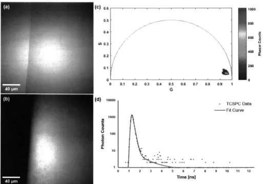
3-1 Fluorescent properties of the sun filter formulation. (a) Trans-illumination image of the edge of a droplet of sun filter formulation, acquired with 755 nm light. (b) TPEF image of the sun filter formulation acquired

with 755 nm excitation light and fluorescence detection from 445 to 480 nm. (c) Phasor plot of the FLIM data associated with (b), high-lighting the short fluorescence lifetime of the sun filter formulation. (d) Temporal decay trace of a typical pixel from (b), illustrating the rapid

decay of the sun filter fluorescence. . . . . 85

3-2 Fluorescence detected from the stratum spinosum layer of the viable epidermis, acquired at a depth of 50 pm below the skin surface. (a) TPEF image of human skin treated with vehicle only, showing

endoge-nous NADH fluorescence. (b) Phasor plot of the FLIM data associated with (a). (c) Temporal decay trace of a pixel from (a), showing the pro-gressive decay of NADH fluorescence. (d) TPEF image of human skin treated with sun filter formulation, showing both endogenous NADH

fluorescence across the field of view, as well as exogenous fluorescence from the sun filters seen in the lower right region of the image. (e)

Phasor plot of the FLIM data associated with (d). (f) Temporal decay

trace of a pixel from (d) with a strong fluorescence contribution from chem ical sun filters. . . . . 86

3-3 Simulation to validate the proposed non-Euclidean separation

algo-rithm. (a) Phasor plot of simulated endogenous fluorescence reference sample. (b) Phasor plot of simulated exogenous fluorescence reference sample. (c) Phasor plot of simulated test image, consisting of both flu-orophores with concentrations varying in opposite sigmoidal fashion.

(d) Simulated endogenous fluorescence contribution to the test image.

(e) Estimation of endogenous fluorescence contribution computed using the traditional Euclidean method. (f) Estimation of endogenous fluo-rescence contribution using the proposed non-Euclidean method based on the Mahalanobis distance. (g) Column-wise means of the images in

(d-f), illustrating the superior accuracy of the proposed method over

the classical Euclidean approach. . . . . 87

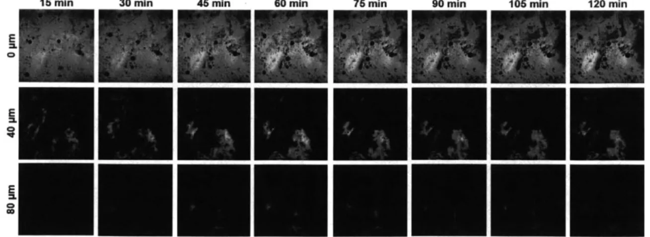
3-4 Comparison of processing methods to optimally determine endogenous fluorescence contribution. (a) TPEF intensity image of human skin treated with chemical sun filters, showing a diffusing pool of formu-lation in the bottom right portion of the image. (b) Estimate of the endogenous fluorescence contribution computed using the traditional Euclidean method. (c) Estimate of the endogenous fluorescence contri-bution as determined by the proposed non-Euclidean approach based on the Mahalanobis distance metric. . . . . 88 3-5 Diffusion of the lipophilic solvent throughout various layers of human

epidermis (0, 40, and 80 pm below the skin surface), as visualized using CARS microscopy to probe the CH2 vibrational mode of Finsolv TN

at 2845 cm 1 at 15-minute intervals over the course of 2 hours. All images are 318 pum x 318 pm in size. . . . . 89 3-6 Fluorescence intensity and computed NORR images of a typical skin

sample. (a) NADH fluorescence intensity. (b) FAD fluorescence inten-sity. (c) NORR image, obtained by computing FAD/(NADH+FAD)

3-7 Normalized optical redox ratio (NORR) of cells in the stratum spinosum

layer of the viable epidermis treated with either vehicle only or sun

fil-ter formulation, and exposed to either 0 or 20 J/cm2 (1 MED) of UVA

irradiation. Bars correspond to mean NORR measurement of cells from N = 3 fields of view, and error bars represent 1 standard

devi-ation. Statistical significance determined by pair-wise Student's t-test

corrected using Holm's method, annotated with * if p < 0.01 and ** if

p < 0.005. . . . . 92

4-1 Phasor plot showing the mean coordinates of phasor clusters A, B, and

C, as well as the phasor of a given pixel X. A line is drawn between

phasor X and the mean coordinates of reference cluster A, where its intersection with the line connecting clusters B and C yields the

coor-dinates of R . . . . 105

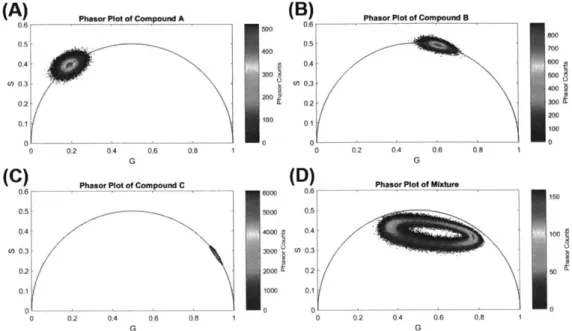
4-2 Phasor plots of the simulated data used to test the accuracy of the

separation algorithms in the context of a binary mixture of

single-lifetime fluorophores. (A) Phasor plot of compound A with a single-lifetime of 4.100 + 0.205 ns. (B) Phasor plot of compound B with a lifetime of

0.200 0.010 ns. (C) Phasor plot of the binary mixture of compounds

A and B . . . . 107

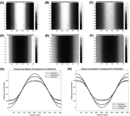
4-3 Estimated concentration maps of either compound in a binary

mix-ture of single-lifetime fluorophores. (A,D) Theoretical concentration maps of compounds A and B, spatially distributed following squared

sine and cosine functions, respectively. (B,E) Concentration maps of compounds A and B, respectively, estimated using the Mahalanobis distance metric. (C,F) Concentration maps of compounds A and B, re-spectively, estimated using the Euclidean distance metric. (G) Column-wise means of panels A-C. (H) Column-Column-wise means of panels D-F. . . 108

4-4 Phasor plots of the simulated data used to test the accuracy of the separation algorithms in the context of a binary mixture of fluorophores with multiple lifetimes. (A) Phasor plot of compound A with a lifetime of 4.100 0.205 ns. (B) Phasor plot of compound B, characterized by

a combination of 4 distinct lifetimes. (C) Phasor plot of the binary mixture of compounds A and B. . . . . 109

4-5 Estimatcd concentration maps of either compound in a binary mix-ture of fluorophores with multiple lifetimes. (A,D) Theoretical concen-tration maps of compounds A and B, spatially distributed following squared sine and cosine functions, respectively. (B,E) Concentration maps of compounds A and B, respectively, estimated using the Ma-halanobis distance metric. (C,F) Concentration maps of compounds

A and B, respectively, estimated using the Euclidean distance metric. (G) Column-wise means of panels A-C. (H) Column-wise means of

panels D -F . . . . 110

4-6 Phasor plots of the simulated data used to test the accuracy of the separation algorithms in the context of a ternary mixture of single-lifetime fluorophores. (A) Phasor plot of compound A with a single-lifetime of 4.100 0.205 ns. (B) Phasor plot of compound B with a lifetime of

1.600 t 0.080 ns. (C) Phasor plot of compound C with a lifetime of

0.600 0.030 ns. (D) Phasor plot of the ternary mixture of compounds

4-7 Estimated concentration maps of each compound in a ternary mix-ture of single-lifetime fluorophores. (A,D,G) Theoretical concentration maps of compounds A, B, and C, respectively, spatially distributed following cosine functions phase-shifted with respect to one another by 27r/3 radians (B,E,H) Concentration maps of compounds A, B, and C, respectively, estimated using the Mahalanobis distance metric. (C,F,I) Concentration maps of compounds A, B, and C, respectively, estimated using the Euclidean distance metric. (J,K,L) Column-wise means of panels A-C, D-F, and G-I, respectively. . . . . 113

5-1 CRS images of human stratum corneum acquired from ex vivo skin ex-plants. (a-c) CARS and (d-f) SRS images of stratum corneum showing (a,d) lipid-weighted content; (b,e) protein-weighted content; and (c,f) water-weighted content. The NRB in the CARS data manifests itself as a homogeneous and unspecific haze distributed across the field of view . . . . 122

5-2 Manual segmentation of SRS lipid content image to distinguish

intra-cellular and extraintra-cellular spaces for subsequent analysis. (a) Unlabeled image. (b) Manually segmented image, showing corneocytes identified

by indices 1 through 22, and extracellular space corresponding to the

surrounding region identified by index number 23. . . . . 123

5-3 Scatter plot of all intracellular lipid and protein data collected via SRS, showing a strong correlation (Pearson's R = 0.921) between the

observed metrics and therefore indicative of spectral overlap. . . . . . 124

5-4 Corneometer measurements obtained from ex vivo human skin through-out the dehydration time course on a plastic substrate (i.e. rapid de-hydration) and a gel substrate (i.e. slow dede-hydration). Data points correspond to the mean of the triplicate corneometer measurements with error bars indicating the standard error of the mean. Statistically significant deviations from the corresponding initial timepoint are de-noted by asterisks and determined via Student's t-test (*: p < 0.05/N;

**: p < 0.01/N; ***: p < 0.001/N, adjusted using Bonferroni

correc-tion with N = 4 pairwise comparisons). . . . . 125

5-5 Corneometry-based assessment of ex vivo human skin hydration

dy-namics during rehydration under various environmental and treatment conditions. Data points correspond to the rate of change of corneome-ter measurements per hour, with error bars showing the 95% confidence interval. For the ambient condition without treatment (control), aster-isks denote rates of change significantly different from zero; for all other conditions, they denote rates of change that are significantly different

from the control (*: p < 0.05; **: p < 0.01; ***: p < 0.001, where p-values are adjusted using Holm-Bonferroni correction with N = 36

m etrics). . . . . 129

5-6 Chemical content dynamics of ex vivo human skin during rehydration

under various environmental and treatment conditions. Data points correspond to the rate of change of CRS imaging metrics per hour, with error bars showing the 95% confidence interval. For the ambient condition without treatment (control), asterisks denote rates of change significantly different from zero; for all other conditions, they denote rates of change that are significantly different from the control (*: p <

0.05; **: p < 0.01; ***: p < 0.001, where p-values are adjusted using

5-7 Morphological dynamics of ex vivo human corneocytes during

rehy-dration under various environmental and treatment conditions. Data points correspond to the rate of change of each spatial metric in mi-crons per hour with error bars showing the 95% confidence interval. Nearest neighbor distances are computed between corneocyte cell cen-ters (NNDCenters) as well as between cell walls (NNDwais). For the ambient condition without treatment (control), asterisks denote rates of change significantly different from zero; for all other conditions, they denote rates of change that are significantly different from the control (*: p < 0.05; **: p < 0.01; ***: p < 0.001, where p-values are adjusted using Holm-Bonferroni correction with N = 36 metrics). . . . . 131

6-1 In vitro monolayer model of ovarian cancer showcasing the fluores-cence of DiR before (a) and after (b) photoconversion, with associated fluorescence spectra summed across the entire field of view (c). . ... 152

6-2 Longitudinal monitoring of an ovarian cancer cell subpopulation of in-terest, seen before (a) and after (b) photoconversion on Day 0. The same field of view was revisited 24 hours (c,d) and 48 hours (e,f) fol-lowing the photoconversion process to monitor the cellular proliferation over time. All scale bars correspond to 100 pm. Images in (a,b,d,f) and (c,e) were acquired at 20x and 10x magnification, respectively. . 153

6-3 3D tumor spheroid of ovarian cancer cells before (a) and after (b)

photoconversion of the topmost peripheral region indicated by the gray box. Two regions of interest (ROI) have been selected within the image, where ROI #1 encompassed photoconverted cells while ROI #2 did not. The corresponding fluorescence spectra are shown in (c), where solid and dashed lines refer to ROIs #1 and #2, and diamonds and

circles refer to before and after photoconversion, all respectively. . . . 155

20

6-4 FACS plot of a cell sample from disaggregated, partially photocon-verted ovarian cancer spheroids (a), and subsequent seeding of sorted non-converted (b) and photoconverted (c) cells. The fluorescence spec-tra from the sorted cells are shown in (d), demonsspec-trating the irre-versible nature of in situ DiR photoconversion . . . . 156

6-5 In vivo longitudinal monitoring of a photoconverted subpopulation of melanoma cells indicated by the gray box in a zebrafish xenograft model following in situ photoconversion. In all images, the eye is lo-cated at the bottom-left of the field of view and was consistently used as a fiducial marker throughout the experimental time course to ensure monitoring of the same area over time. The top row shows a colored overlay of the two collected fluorescence emission bands, namely

650-690 nm in green and 760-800 nm in red. The middle row shows a

scatter plot of each pixel, where green and red channel intensities are plotted against one another in order to generate a representation visu-ally reminiscent of flow cytometry plots. The red dashed lines in the scatter plots correspond to the gating criteria to identify pixels con-taining either photoconverted or standard DiR. These gates are then used to recolor the images from the top row, where the images in the bottom row show photoconverted and standard DiR fluorescence in green and red, respectively . . . . 157

7-1 Synthetic pheomelanin in a 4:1 water:hexane emulsion. (a) CARS

image acquired at WpWs = 2000 cm-1. Pheomelanin is observed as

small, insoluble aggregates with bright CARS intensity. The surround-ing water/hexane bubbles show low-level non-resonant CARS back-ground. (b) Trans-illumination image acquired with the 861 nm pump beam. (c) CARS spectrum of synthetic pheomelanin referenced to the wavelength-independent non-resonant signal from a glass cover-slip, normalized by area under the curve. Three synthetic pheomelanin samples were measured, with each spectrum shown in gray; the curve in red corresponds to the mean of the three measurements. . . . . 163

7-2 Melanocytes isolated from red-haired C57BL/6 (Mclre/e, Tyr+/+) mice

exhibit strong CARS signal at Wp - ws = 2000 cm-1. (a)

Trans-illumination image acquired with the pump beam, where the overall shape of the cells can be well visualized. (b) Confocal fluorescence image of tdTomato. (c) False color (Green fire blue colormap in Im-ageJ) CARS image mapping intracellular pheomelanin distribution.

(d) 4x-zoomed view of (c) showing a perinuclear distribution of signal

intensity, consistent with the known biology of protective melanin caps. 165

7-3 Melanocytes isolated from albino-red C57BL/6 (Mclre/e Tyrc/') mice

exhibit negligible CARS signal at Wp - ws = 2000 cm-'. (a)

Trans-illumination image acquired with the 861 nm pump beam. (b) Confocal fluorescence image of tdTomato. (c) False color CARS image acquired with pump (Ap = 861 nm) and Stokes beams (As = 1040 nm). (d)

False color image acquired only using the pump beam, showing promi-nent two-photon fluorescence signals from tdTomato. (e) False color image acquired only using the Stokes beam, showing weak two-photon fluorescence signals from tdTomato. (f) False color image illustrating the true CARS signal obtained by subtracting tdTomato fluorescence in (d) and (e) from the raw CARS image in (c). . . . . 166

7-4 Imaging of pheomelanin stores in red-haired mouse ear skin. (a,c,e) Brightfield trans-illumination image acquired from the microscope eye-piece. (b,d,f) Maximal projection view of CARS image stack of the mouse ear, showing bright granules from the pheomelanin stores (red circles) within melanocytes and at the base of the hair follicle. A CARS

image stack acquired with the pump beam set to 871 nm (wp - Ws =

1866 cm-1) was subtracted from the image stack acquired with the

pump beam set to 861 nm (Wp - Ws = 2000 cm-1) to minimize the

non-resonant signal contribution from structures other than pheome-lanin. Image stacks are 27 pm thick, with a step size of 1 pm. Note that an out-of-focus hair (blue arrow) caused a shadow in the trans-illumination image (a), whereas CARS is highly depth-resolved; there-fore, the hair was not prominently seen in (b). . . . . 167

7-5 Imaging of pheomelanin stores in a red-haired mouse ear in vivo. (a)

Brightfield trans-illumination image acquired from the microscope eye-piece. (b) Maximal projection view of CARS image stack of the mouse ear, showing bright signals from pheomelanin (red circle). A CARS im-age stack acquired with the pump beam set to 871 nm (Wp -is = 1866

cm-1) was subtracted from the image stack acquired with pump beam

set to 861 nm (wp -ws = 2000 cm-') to minimize the non-resonant sig-nal contribution from structures other than pheomelanin. The image

7-6 Imaging of pheomelanin stores in a red-haired (C57BL/6 (Mclr'/e, Tyr+/+) mouse ear section (5 pm thickness). (a) Immunohistochemi-cal stain of the mouse ear slide using anti-Sox-10 antibody (counter-stain: haematoxylin), revealing melanocytes in red, some of which are indicated by black arrows for added clarity. (b) Image of an adjacent unstained 5 pm thick slide under brightfield illumination, revealing pheomelanin-rich deposits (shown by black arrows) consistent with the localization of the melanocytes in the adjacent slide shown in (a). (c) Trans-illumination image of the unstained slide shown in (b) acquired with the pump beam set to 861 nm. (d) CARS and (e) SFA images of the unstained slide shown in (b), revealing bright granular signals from pheomelanotic stores consistent with positive staining in (a) and pigmented areas in (b). (f) False-color overlaid image of (d) in green and (e) in red. A CARS image acquired with the pump beam set to 871 nm (Wp - Ws = 1866 cm-1) was subtracted from the image

ac-quired with the pump beam set to 861 nm (wp - Ws = 2000 cm- 1) to

minimize the non-resonant signal contribution from structures other than pheom elanin. . . . . 169

7-7 Imaging of pheomelanin stores in a red-haired mouse ear section (5 pm

thickness). (a) Brightfield trans-illumination image of the haematoxylin-stained mouse ear slide. (b) Magnified view of the area marked by a red square in (a). Pheomelanotic stores are seen as slightly pigmented granules. (c) CARS image of the same field of view as (b), showing bright granular signals from pheomelanotic stores corresponding to the pigmented areas in (b). A CARS image acquired with the pump beam

set to 871nm (wp - Ws = 1866 cm-1) was subtracted from the image

acquired with the pump beam set to 861 nm (Wp - Ws = 2000 cm 1)

to minimize the non-resonant signal contribution from structures other than pheom elanin. . . . . 170

24

7-8 Imaging of human amelanotic melanoma. (a) Clinical photograph of one amelanotic melanoma lesion. (b) H&E stain of the patient slide (10 x magnification). (c) Perilesional skin showing normal architecture

of both epidermis and dermis. (d) Brightfield trans-illumination image

acquired from the microscope eyepiece from the perilesional area. (e) CARS image of the same perilesional area compared to (d) (image

ac-quired with pump beam wavelength at 841 nm (Wp - Ws = 2275cm 1)

was subtracted from the image acquired with pump beam wavelength

at 855 nm (wp - ws = 2081 cm-1) to minimize the non-resonant

back-ground from structures other than pheomelanin). (f) View of the ame-lanotic melanoma area showing high density of cells with no obvious sign of melanin. (g) Brightfield trans-illumination image acquired from the microscope eyepiece from an unstained slide of the melanoma area, showing slightly pigmented granular structures (red circle). (h) CARS image of the same tumor area compared to (g), with the same settings as for (e). Saturated bright pheomelanin signals were found (red circle) corresponding to the minimally pigmented region shown in (g). (i,j,k) Respectively H&E, trans-illumination, and CARS images of the tu-mor area of slides from a second amelanotic melanoma patient. Strong pheomelanin signals were again observed (red circles). . . . . 172

26

List of Tables

2.1 Summary of cancers diagnosed using various Raman techniques and selected representative associated references. Please note that this list is not meant to be absolute or all encompassing. . . . . 48 2.2 Common Raman band assignments used in cancer diagnostic studies

[1,

3.1 Composition of sun filter formulation . . . . 77 5.1 Stratum corneum metric dynamics measured over the time course of

ex vivo human skin dehydration on two different substrates. For the plastic substrate, asterisks denote rates of change significantly different from zero; for the gel substrate, they denote rates of change that are sig-nificantly different from the plastic substrate (*: p < 0.05; **: p < 0.01;

***: p < 0.001, where p-values are adjusted using Holm-Bonferroni

cor-rection with N = 36 metrics. IER: intracellular-to-extracellular ratio;

NND: nearest neighbor distance; CI: confidence interval.) . . . . 128

5.2 Summary of observed changes over the time course of skin explant rehydration. (N/C: no change;

+++,

+:

28

Chapter 1

Theory and Principles of Nonlinear

Optics for Biomedical Imaging

1.1

Introduction

Prior to understanding the fundamentals of nonlinear optics, it is a useful exercise to consider what is meant by linear optics. When a material is exposed to an electric field

79

9 ~, foxN(1.1)

The proportionality is defined by Eo, a universal constant known as the permittiv-ity of free space, and x, the material's electric susceptibilpermittiv-ity. This linear relationship implies superposition; that is, the polarization response of a material exposed to a sum of fields simply corresponds to the sum of the polarization responses to each field considered individually. In addition, this also implies that the incident fields cannot interact with one another to generate new frequencies at the system's output. This is a relation commonly introduced in most introductory optics and/or electromagnetic fields classes in undergraduate science and engineering programs; however, this equa-tion is but a simple and convenient approximaequa-tion. In reality, nonlinear polarizaequa-tion

responses do exist - they simply require an enormous amount of incident power in order to generate a detectable signal as a result of the vanishingly small nonlinear electric susceptibility coefficients. In fact, this is because the susceptibility x of a given material can be represented by a Taylor series expansion, where nonlinear ma-terial properties emerge with incident fields that are sufficiently strong. This relation is shown more clearly in Equation 1.2. Considering the large amount of input energy that is required to elicit this nonlinear optical polarization responses however, an ensuing question naturally arises: if extremely high irradiation powers are required to induce nonlinear optical polarizations, how are nonlinear optical signals generated in biological samples in a non-destructive manner? The answer lies in the use of ultrafast laser sources.

7P

(1.2)

These are laser systems that, instead of emitting a constant beam of coherent light (unlike continuous wave, or CW, laser sources), emit extremely short - but extremely powerful - pulses of light. These short pulse durations can range from a few nanoseconds all the way down to the femtosecond regime. In the case of the various studies documented in the context of the present thesis, the Spectra-Physics InSight DeepSee - a commercial femtosecond laser source - is the laser source of choice. One output can be selectively tuned from 680 up to 1300 nm in single-nanometer increments, while the other is fixed at 1040 nm. The concurrent use of two laser beams will become clear in the context of particular nonlinear optical imaging applications that will be presented in depth in Sections 1.4.2 and 16. The pulse durations are about 120 fs in duration, and the laser has a repetition rate of 80 MHz. This also implies an interpulse period of 12.5 ns, which implies that when the laser is in operation, no light is being emitted 99.999% of the time. However, for the brief 0.001% of the time where a pulse is emitted, it propagates with a peak power exceeding 100 kW. The time-averaged power for the laser source nevertheless remains in the milliwatt range, thereby minimizing photodamage. It is also worth specifying

that for nonlinear optical imaging, the photon density is crucial factor to consider from an imaging standpoint. That is, not only does one require kilowatt-range peak powers, but this energy must also be focused into a small focal volume in order to generate any appreciable signal. This is conveniently advantageous, because it is this property that ensures the "intrinsic optical sectioning" that is a hallmark of nonlinear optical microscopy.

These intrinsic properties of nonlinear optical microscopy eliminate the need for a confocal pinhole as in the case of single-photon confocal fluorescence microscopy, for example, used to suppress the out-of-focus light. Given that the signal is strictly generated at the focus of the microscope objective, full 3D volumetric reconstructions of biological samples can be achieved by simply scanning the objective focus across the X, Y, and Z dimensions.

With this introductory framework for nonlinear optics in mind, the following sec-tions will build on these foundasec-tions, ranging from two-photon excitation fluorescence (TPEF) to coherent Raman scattering (CRS) to sum-frequency and transient absorp-tion (SFA and TA) imaging techniques.

1.2

Two-Photon Excitation Fluorescence (TPEF)

Two-photon excitation fluorescence (TPEF) is a nonlinear optical interaction whereby two photons are simultaneously absorbed by a molecule in order to generate a sin-gle output photon. This nonlinear optical phenomenon was first implemented as a microscopy technique back in 1990 by Denk and colleagues [9]. It is worth noting, however, that because TPEF requires the simultaneous absorption of two incident photons, this nonlinear optical effect is symmetry-forbidden in non-centrosymmetric molecules. This is because materials and molecules that exhibit inversion symmetry (i.e. compounds that are centrosymmetric) have even-ordered nonlinear electric sus-ceptibilities equal to zero. Nevertheless, even-ordered nonlinear optical effects may still be generated in such media by breaking its symmetry. This can be done by cou-pling with the molecule's vibrational and/or rotational modes with odd symmetry in

order to enable excitation.

It is also worth noting that TPEF is not a lossless process. Upon the simultaneous absorption of two incident photons by a molecule, there is some non-radiative decay, followed by a transient residency in an excited electronic state for a given period of time T called the fluorescence lifetime, finally resulting in the emission of a fluorescent

photon as the molecule returns to its ground state. In addition, two-photon excitation spectra are more complex than simply doubling the wavelength of the single-photon excitation spectrum. This discrepancy is due to differences in Frank-Condon factors, which can be better appreciated by taking a look at the 1- and 2-photon spectra of common fluorophores. Moreover, because TPEF is a X process, the signal intensity

is proportional to the square of the incident power, i.e. 12(t).

1.3

Fluorescence Lifetime Imaging Microscopy (FLIM)

Fluorescence lifetime imaging microscopy (FLIM) can be viewed as an extension TPEF when implemented in a two-photon setting, whereby the fluorescence lifetime

T of a given fluorophore can be probed in addition to its intensity [10]. In addition to probing the optical properties of fluorophores (i.e. excitation and emission param-eters), FLIM is a tool also capable of probing their temporal dynamics. To this aim, this imaging technique requires specific hardware (i.e. time-correlated single photon counting, or TCSPC), and the resulting data can be processed either in the time domain or in the frequency domain, the latter of which is typically performed using phasor analysis. FLIM is therefore an extremely useful modality in the context of molecular imaging, as it provides researchers with an additional dimension of imaging contrast [11].

1.3.1

Time-Correlated Single Photon Counting (TCSPC)

The implementation of FLIM relies on the operating principles of time-correlated sin-gle photon counting (TCSPC) [12]. In such a case, the detector (i.e. photomultiplier tube, or PMT) is connected to pre-amplifier, which is in turn connected to the

SPC module. For multiple detectors, the each PMT pre-amplifier is first connected to

a routing block before the TCSPC module, whereby the PMTs independently emit an electronic impulse signal at each photon detection event for multiplexed detection. In parallel, a synchronization module registers the timing of the laser excitation pulse. In turn, the time-to-amplitude converter (TAC) measures the time difference between the arrival of the detected photon and the emission of the following excitation laser pulse. The difference between this measured time interval and the laser repetition period (given by the inverse of the pulse repetition frequency, an intrinsic property of the laser source) corresponds to the fluorescence emission delay for that particular photon. The hardware network has an overall dead time on the order of 100 ns or so [12]; for this reason, each incident laser pulse must result in the detection of at most 1 fluorescence photon per detector in order to limit lifetime biasing towards shorter values. In other words, this implementation of TCSPC for FLIM does not al-low for over-counting of photons, which would otherwise result in inaccurate lifetime measurements.

Once the FLIM data is acquired using the TCSPC techniques described above, each pixel of the acquired XYT dataset can be analyzed using either time-domain or frequency-domain analysis - the latter of which is most commonly referred to as

"phasor analysis".

1.3.2

Time-Domain Analysis

Time-domain analysis of FLIM data typically involves curve fitting of fluorescent decay traces on a pixel-by-pixel basis using a sum of exponential decays. In such a context, each fluorophore of a given decay trace is characterized by its respective time constant Ti and relative weight aj, defining its contribution to the overall fluorescence signal in the pixel in question. The relation between a pixel's temporal decay trace

(t) and the fluorophores therein is summarized in Equation 1.3.

N

I(t) = aie- (1.3)

As will be discussed in further detail in Chapter 4, time-domain analysis requires a fair bit of familiarity with the sample at hand. This encompasses not only the number of compounds to distinguish, but also an a priori idea of their respective fluorescent lifetimes [13]. To complicate matters further, there is an added dimen-sion of complexity when imaging cellular and tissue autofluorescence, including flavin and nicotinamide adenine dinucleotides (FAD and NADH, respectively). Such com-pounds naturally exhibit multiple lifetimes, which in turn vary based on their molec-ular conformation and binding states [14, 15, 16]. Bearing in mind that time-domain analysis is based on iterative curve fitting, the task of resolving multiple sources of fluorescence that themselves have multiple lifetimes rapidly becomes computation-ally demanding. To add to the present challenge, accurate time-domain analysis of fluorescence lifetimes often requires a prohibitively large number of photon counts per pixel (typically exceeding 5000 photons), particularly when the fluorescence from one compound dwarfs the other [13]. This requirement is due to shot noise (also known as Poisson noise), which is related to the particle nature of light. Consider-ing that photon emission can be described as a Poisson process, the signal-to-noise ratio (SNR) is given by SNR = N/v = v , where N is the number of detected photons. Such elevated photon counts inherently demand longer acquisition times and/or higher laser excitation power. However, due to the fragile nature of typical biological samples, these imaging parameters may be incompatible with specimens of interest - particularly living samples.

1.3.3

Phasor Analysis

As an alternative to time-domain analysis, frequency-domain analysis - more com-monly referred to as phasor analysis - is much less demanding in terms of prior sam-ple knowledge [17]. Moreover, this approach yields an intuitive and convenient visual interpretation of the sample data. Instead of performing curve fitting on a pixel-by-pixel basis, phasor analysis involves a simple mathematical transform of each pixel-by-pixel's temporal decay trace. This transformation, related to the Fourier transform, yields a pair of coordinates (G, S) that describe a so-called phasor, which is characterized

34

by its modulus M = 2 S2 _{and phase angle}

#

phasor coordinates (G, S) are obtained by computing the real and imaginary compo-nents of the Fourier transform of the temporal decay trace evaluated at the angular laser repetition frequency w, normalized by its area under the curve. These relations

are summarized in Equations 1.4 and 1.5.

100 1(t) cos(wt)dt G = 00 (1.4) fo I (t) dt -

f

The angular frequency is defined by w = 27rf, where

f

f

[17].

(G - 0.5)2 + S2 = 0.25 (1.6)

In the FLIM community, this is referred to as the universal semicircle. In the case of a decay trace characterized by two fluorescence lifetimes, the transformed phasor coordinates lie along a line connecting the two individual lifetimes on the universal semicircle. The specific phasor coordinates along that line in turn depend on the relative contributions of either fluorescent compound [17, 18]. Given a mixture of fluorescent compounds, FLIM data analysis in the phasor domain therefore

conve-niently offers the ability to estimate the relative fluorescence contribution of each compound at every pixel in the image based on the relative distances between each pixel's corresponding phasor location and the respective reference phasor clusters of the fluorophores at hand.

1.4

Raman Scattering

There are a wide variety of coherent Raman scattering (CRS) techniques, but for the purposes of the present discussion, the fundamentals of spontaneous Raman scattering will first be discussed, follow by an overview of two of the most commonly used implementations of CRS, namely coherent anti-Stokes Raman scattering (CARS) and stimulated Raman scattering (SRS).

1.4.1

Spontaneous Raman Scattering

Raman scattering is a non-parametric process related to the interaction of light with a molecule and its associated vibrational states. This process was discovered by Sir Chandrasekhara Venkata Raman in 1928, when he observed the scattering of an entire spectrum of light upon illumination of a sample with monochromatic light of frequency Wp. As he expected, the most prominent feature of the spectrum occurred at the incident light frequency Wp, which is attributed to an elastic interaction known as Rayleigh scattering. However, weak spectral lines were also observed, which were later understood to occur as a result of inelastic interactions between incident photons and the molecular vibrations present in a sample. As energy is transferred during this process, the spectral lines had shifted frequencies Wp WR, corresponding to what are now known as Stokes (Wp - wR) and anti-Stokes shifts (Wp + WR). Raman observed that these shifts and their resulting spectra were highly material specific a discovery that was awarded the 1930 Nobel Prize in physics. It is worth noting that in most use cases, the incident field at Wp is within the visible or infrared range of the electromagnetic spectrum, while the molecular vibrations themselves can be directly probed at wR that lie in the mid- or long-wavelength infrared ranges.

Fundamentally, Raman scattering is derived from interactions with the time-varying electromagnetic field of light and the time-time-varying electric polarizability caused by molecular vibrations. When a molecule interacts with a photon, it can experience an instantaneous coupling with the photon's electric field, leading to a polarization of the molecule. This coupling can result in the creation of a scattered

photon at frequency Wp - WR if some of the energy from the incident light is con-verted to drive the molecular vibration; it is scattered at WP + wR if the molecule is already in an excited vibrational state, whereupon the scattered photon exits with energy equal to the sum of those of the incident photon and the molecular vibration.

These interactions at Wp - WR and WP + WR correspond to Stokes and anti-Stokes

shifts, respectively. However, this process is far from efficient, as the creation of a frequency-shifted photon hinges on an infrequent interaction with the vacuum field. Given that a spontaneous emission process is defined by the creation of a photon in a previously unoccupied mode, this Raman process is deemed spontaneous [19].

It should be noted that Raman transitions depend on the rate of change of polar-izability with respect to the molecule's geometry. This implies that Raman scattering is only possible for certain symmetries of molecular vibrations, which forms the basis for the so-called selection rules for Raman scattering. While the formalism here pre-dicts the existence of Stokes and anti-Stokes frequency components, it fails to consider the strength of individual Raman transitions, which would otherwise require a more elaborate quantum mechanical formalism that is beyond the scope of the present discussion. The reader is encouraged to refer to the textbook by Long for a more rigorous quantum mechanical approach to the principles of Raman scattering [20].

It is also worth noting that there exists a mechanism whereby the Raman scat-tering response of a molecule can be increased by several order of magnitude, known as surface-enhanced Raman scattering (SERS), which involved adsorption of the molecule onto a roughened or nano-sized metallic substrate. Metallic or plasmonic nanoparticles are known for their unique interaction with light that results in the excitation of their localized surface plasmon resonance (LSPR). LSPR excitation re-sults in not only enhanced light absorption and scattering from the nanoparticle, but also produces an enhanced electromagnetic field around the surface of the

nanopar-ticle that can be readily exploited for Raman enhancement [21, 22, 23, 24]. When

a molecule is adsorbed onto or is within close proximity of the nanoparticle surface,

the EM field felt by the molecule is that of the incident field and the enhanced EM field at the nanoparticle surface. While the in-depth discussion of SERS is beyond

the scope of the present thesis work, a more detailed mathematical description of plasmonic nanoparticle Raman signal enhancement can be found in several excellent texts by Van Duyne and colleagues [21, 231.

1.4.2

Coherent Raman Scattering (CRS)

Coherent Raman scattering is a term that refers to a class of stimulated interactions where Raman processes are driven coherently, leading to the generation of strong scattering signals. This differs from traditional Raman scattering, which is depen-dent on spontaneous interactions. As was previously mentioned, spontaneous Raman scattering depends on an infrequent interaction with the vacuum field. In coherent Raman scattering, two light fields are introduced into a sample that have an energy difference equal to a molecular vibration of interest. These two fields act to stimulate, or drive, the Raman process, increasing its efficiency by several orders of magnitude

[19].

Though many types of coherent Raman scattering processes have been discovered and developed [25, 26], two types of coherent Raman scattering have been specifically developed towards biomedical applications: stimulated Raman scattering (SRS) and coherent anti-Stokes Raman scattering (CARS). Both mechanisms of signal genera-tion are so-called "four-wave mixing" processes, which implies that incident photons interact with the material's vibrational properties to produce scattering contrast that can be used for imaging. Important distinctions exist between CARS and SRS how-ever, resulting in differences in detection schemes and image contrast. Schematically, the energy diagrams for spontaneous Raman scattering, SRS, and CARS are pre-sented in Figure 1-1.

Conceptually, SRS and CARS both involve the use of two incident fields at fre-quencies Wp and ws, respectively referred to as the pump and Stokes beams, where the difference between these two frequencies is tuned to match a molecular vibration of interest. In the case of SRS, the introduction of electric fields at both frequen-cies allows for a transfer of photons at the pump frequency to photons at the Stokes frequency due to coupling with the sample's endogenous molecular vibrations. This

38

A

B

C

WWA

Wp

WS

Wp

WS

Wp

Wp

Spontaneous SRS CARS

Figure 1-1: Schematic representation of the fields involved in Raman scattering pro-cesses. (A) Spontaneous Raman scattering, (B) stimulated Raman scattering (SRS),

and (C) coherent Stokes Raman scattering (CARS). The pump, Stokes, and

anti-Stokes frequencies are respectively designated by Wp, ws, and WAS, while the dashed

and solid lines respectively refer to virtual and real molecular states. In spontaneous

Raman scattering, a pump photon scatters inelastically, thus generating a Stokes pho-ton. In SRS, both pump and Stokes fields are incident on the sample simultaneously; if there is a vibrational band gap that corresponds to the energy difference between the two beams, the pump field decreases (stimulated Raman loss, SRL), while the Stokes field is amplified (stimulated Raman gain, SRG). Finally, in CARS, a new field is created at the anti-Stokes frequency and can be readily detected via optical filters, as it is blue-shifted relative to the incident pump and Stokes fields.

implies that the pump beam intensity decreases in the presence of a Raman-active molecule, while that of the Stokes beam increases. In order to pick up this small

energy transfer, SRS microscopy is achieved either by detecting the decrease in pump

intensity (stimulated Raman loss, SRL) or the increase in Stokes intensity (stimulated Raman gain, SRG).

SRL is achieved through high-frequency modulation (typically on the order of several MHz to circumvent laser noise and improve both imaging speed and detection sensitivity [27]) of the Stokes beam via an acousto-optic or electro-optic modulator (AOM and EOM, respectively). This implies that the SRS signal will manifest itself

as a high-frequency modulation superimposed onto the intensity of the pump beam

(Figure 1-2). Detection thus requires the use of a lock-in amplifier (LIA) or demod-ulation to isolate the high-frequency component of the pump intensity. Conversely,