Assembly and operation of the autopatcher for automated intracellular neural recording in vivo

Assembly and operation of the autopatcher for

automated intracellular neural recording in vivo

The MIT Faculty has made this article openly available.

Please share

how this access benefits you. Your story matters.

Citation

Kodandaramaiah, Suhasa B, Gregory L Holst, Ian R Wickersham,

Annabelle C Singer, Giovanni Talei Franzesi, Michael L McKinnon,

Craig R Forest, and Edward S Boyden. “Assembly and Operation of

the Autopatcher for Automated Intracellular Neural Recording in

Vivo.” Nature Protocols 11, no. 4 (March 3, 2016): 634–654.

As Published

http://dx.doi.org/10.1038/nprot.2016.007

Publisher

Nature Publishing Group

Version

Author's final manuscript

Citable link

http://hdl.handle.net/1721.1/107907

Terms of Use

Creative Commons Attribution-Noncommercial-Share Alike

Setting up and using the autopatcher for automated intracellular

neural recording in vivo

Suhasa B. Kodandaramaiah1,2,3, Gregory L. Holst4, Ian R. Wickersham1,2,3, Annabelle C. Singer1,2,3_{, Giovanni Talei Franzesi}1_{, Michael L. McKinnon}5_{, Craig R. Forest}4,*_{, and Edward}

S. Boyden1,2,3,*

1_{MIT Media Lab, MIT, Cambridge, MA}

2_{McGovern Institute for Brain Research, Cambridge MA}

3_{Depts. of Biological Engineering and Brain and Cognitive Sciences, MIT, Cambridge MA} 4_{George W. Woodruff School of Mechanical Engineering, Georgia Institute Of Technology,} Atlanta, GA

5_{Department of Physiology, School of Medicine, Emory University, Atlanta, GA}

Abstract

Whole cell patch clamping in vivo is an important neuroscience technique that uniquely provides access to both supra-threshold spiking and sub-threshold synaptic events of single neurons in the brain. This article describes how to set up and use the autopatcher, a robot for automatically obtaining high yield and high quality whole cell patch clamp recordings in vivo. Following this protocol, a functional experimental rig for automated whole cell patch clamping can be set up in one week. High quality surgical preparation of mice takes approximately 1 hour, and each autopatching experiment can be carried out over periods lasting several hours. Autopatching should enable in vivo intracellular investigations to be accessible by a significant number of neuroscience labs, and enable labs already doing in vivo patch clamp to scale up their efforts by reducing training time for new lab members and increasing experimental durations by handling mentally intensive tasks automatically.

INTRODUCTION

In vivo whole cell patch clamping is an electrophysiological technique that enables high-fidelity measurement of the electrical activity of neurons in the living brain. The high

Correspondence to: Craig R. Forest, G. W. Woodruff School of Mechanical Engineering, Georgia Institute of Technology, 813 Ferst

Dr, Room 411, Atlanta, GA 30332, ; Email: cforest@gatech.edu, Office phone: (404) 385-7645; and Edward S. Boyden, MIT Media Lab, McGovern Institute, Dept. of Biological Engineering, and Dept. of Brain and Cognitive Sciences, Massachusetts Institute of Technology, 20 Ames St, E15-421, Cambridge, MA 02139, ; Email: esb@media.mit.edu, Office phone: (617) 324-3085

AUTHOR CONTRIBUTIONS

SBK, IRW, GLH, CRF, and ESB designed, built and tested the autopatcher system. ACS and GTF assisted with experiments. MLK developed the software included with the manuscript. SBK, IRW, GLH, ACS, GTF, CRF and ESB wrote the manuscript.

CONFLICT OF INTEREST

HHS Public Access

Author manuscript

Nat Protoc

Published in final edited form as:

Nat Protoc. 2016 April ; 11(4): 634–654. doi:10.1038/nprot.2016.007.

A

uthor Man

uscr

ipt

A

uthor Man

uscr

ipt

A

uthor Man

uscr

ipt

A

uthor Man

uscr

ipt

signal–to-noise ratio and temporal resolution of the recordings enables the measurement of both subthreshold membrane potentials and suprathreshold spiking events1–4. Moreover, current can be delivered intracellularly to drive or silence the cell being recorded or to allow characterization of specific receptors or ion channels in the cell. In addition, whole cell patch clamping allows infusion of cell staining dyes to visualize cell morphology, extraction of cell contents for transcriptomic analysis5 and single cell gene transfection6. Since its early application for recording in vivo7, it has been a gold standard technique for the study of intracellular dynamics of single neurons in intact brains1, 8–16. It has also been combined with two-photon imaging for targeted patch clamping of identified neurons17–19. Multiple groups have demonstrated the use of in vivo patch clamping for recording in awake freely moving animals20–23. However, manual whole cell patch clamping is a laborious technique and is considered something of an art form, especially when performed in vivo. Manual whole-cell patch clamping has proven difficult to automate, and therefore has had low yield and throughput. We recently discovered a different method for in vivo patch clamping that was simple to automate24. In our method, we detect neurons by lowering a pipette in small (e.g., 2 μm) steps, and perform a time series analysis of the resistance of the patch pipette as it is lowered into the brain, looking for a small, but monotonic, increase in pipette resistance that takes place over several consecutive steps. This differs from previous methods of neuron detection in vivo, which utilize human-detectable changes, e.g. large jumps in resistance, or appearance of fluctuations in the pipette signals due to heartbeat7, 25, and may contribute to the high performance of our method when performed in an automated fashion. This protocol article provides further practical details on setting up the autopatcher, as well as the

procedure for using the autopatcher to obtain whole cell recordings in the live mammalian brain.

Automating in vivo whole cell patch clamp

The autopatching algorithm breaks down the process of whole cell patch clamping into six stages (Fig. 1a). The autopatcher conducts an initial assessment of the suitability of an installed pipette for patch clamping (‘Pipette assessment outside the brain’). Then the autopatcher rapidly lowers the patch pipette to the desired recording area (‘Regional pipette localization’) with the pipette interior at high positive pressure to prevent tip clogging. This is followed by the ‘Neuron hunting’ stage, in which the pipette is advanced in small increments at a lower pressure while constantly monitoring the pipette resistance until a neuron is detected, as indicated by a specific temporal sequence of pipette resistance changes. Once a neuron has been detected, the ‘Gigaseal formation’ stage is executed, during which negative pressure and hyperpolarizing current are applied to the pipette to attempt to form a seal with the targeted cell’s membrane. Finally, in the ‘Break-in’ phase, brief pulses of negative pressure and/or voltage are applied to rupture the patch of membrane at the pipette tip to obtain the whole-cell configuration.

The autopatcher executes this algorithm by assuming position, pneumatic and electric control of the patch pipette (Fig. 1b). Position control of the patch pipette is achieved by using a programmable linear motor. A “digitizer” board equipped with analog inputs, as well as analog and digital outputs, in a custom-built control box interfaces with the patch

amplifier to acquire and log pipette impedance measurements throughout the autopatching

A

uthor Man

uscr

ipt

A

uthor Man

uscr

ipt

A

uthor Man

uscr

ipt

A

uthor Man

uscr

ipt

process, and controls the application of hyperpolarizing current during gigasealing. The control box also includes an electronic pressure regulation system that can apply positive and negative pressures to the pipette at various stages of autopatching. Included with this protocol is the autopatcher software (Supplementary Data 1), which executes the algorithm. The success rates seen when using our robot are similar to those obtained by trained humans. Whole cell patch clamping in anesthetized mice is successful in ~32% of the trials on average, with greater than 60% of the trials yielding good recordings in a freshly opened craniotomy24. Thus, for investigators starting to do in vivo whole cell patch, our robot may facilitate entry into the field. Robots do not suffer from fatigue and may thus be of use even for trained in vivo patch clamp electrophysiologists seeking to increase robustness and yield for lengthy experiments.

Overview of autopatcher hardware and software

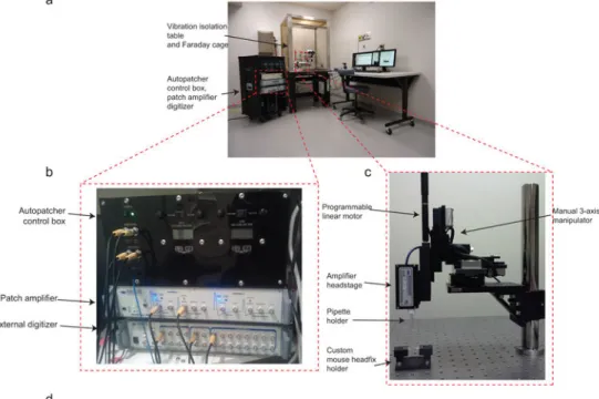
The general layout of the autopatcher equipment is shown in Figure 2. The core components of the autopatcher setup include the patch amplifier, a signal digitizer board equipped with analog inputs, as well as analog and digital outputs, for data acquisition and control, a custom autopatcher control box, and a pipette actuator for manipulating the patch pipette. The pipette actuator along with the amplifier headstage and custom head fixation base for immobilizing the mouse are installed on an optics table (or other sturdy table that is isolated from mechanical vibrations and electrical noise) (Fig. 2a and c). The pipette actuator allows programmatic control of the patch pipette movement in the axial direction during

autopatching. In the current implementation (Fig. 2c) this is achieved by mounting a programmable linear motor (PT1-Z8 motor with TDC001 controller, Thorlabs) onto a manually controlled 3-axis linear stage (MPC285, Sutter Instruments).

The autopatcher equipment described here has been improved over that described in 2012. The key difference between the current version and the original 2012 version24 is the use of an electronic control box instead of a manual syringe for pressure control. This control box also interfaces with the patch amplifier and the traditional external data acquisition device/ digitizer (required for patch clamp amplifier operation; Fig. 2b and d). The control box takes in a steady high pressure air supply (~2580 mBar) and downregulates it to two discrete positive pressures (high positive pressure of 1000 mBar and low positive pressure of 100 mBar). Two discrete negative pressures states (high negative pressure of −350 mBar and low negative pressure of −25 mBar) are also generated from the same steady high-pressure air input using Venturi tube vacuum generators. Finer control of these pressures is then achieved by using electronic pressure regulators which can modulate the pressures (0 to 800 mBar high positive pressure, 0 to 25 mBar low positive pressure, −25 to 0 mBar low negative pressure and −350 to 0 mBar high negative pressure) using potentiometers mounted on the control box’s front panel. These pressures are inputs to a bank of 3-way valves. Digital TTL signals from the digitizer board switch the individual valves to change which pressure is applied to the pipette during autopatching.

The digitizer board inside the control box connects to the computer via a USB interface. It has one analog output channel dedicated to sending command signals to the patch amplifier during autopatching. An internal relay is used to switch the command signals sent to the

A

uthor Man

uscr

ipt

A

uthor Man

uscr

ipt

A

uthor Man

uscr

ipt

A

uthor Man

uscr

ipt

amplifier from the internal digitizer or the traditional external digitizer to enable

experimental flexibility (Fig. 2d). One analog input channel is used to record the current or voltage output signal from the patch amplifier. These measurements are used to compute the pipette resistances while the autopatching algorithm is being executed. The amplifier output is split within the box and routed to the traditional external digitizer as well as the internal one. These improvements in the pressure delivery system necessitated changes to the 2012 software interface. While the algorithm used for autopatcher is the same as that described in our 2012 paper24, the software has been modified to interface with the new hardware configuration. The current software program also includes scripts for controlling the amplifier software within the autopatcher program using dynamic link libraries (.dll) (Supplementary Data 1). Some of the materials included in this protocol (specifically, the software) were previously posted at the website http://autopatcher.org; going forward, we will post periodic updates to the software and hardware on this site.

The rationale for including an extra linear motor, in addition to the software-controllable Sutter manipulator, and an internal digitizer, in addition to the traditional external digitizer, is to enable modularity. That is, we wanted to design a system that could be added easily to an existing patch rig, to make it automated. Of course, motors that can be directly controlled by computer (for example the Sutter manipulator) or external digitizers that allow external software access, may be directly modified by end users, and in such cases one could ignore the additional motor and digitizer. But here we focus on a modular toolbox that, in principle, could be added to any existing patch system to make it automated.

Experimental Design

The protocol for setting up an autopatcher and performing automated whole cell patch clamping in vivo is divided into six stages. Stage I – Hardware Setup has detailed

instructions for constructing, calibrating and testing autopatcher-specific hardware (Steps 1–

6). This is followed by Stage II – Software Setup which guides the user on configuring the

autopatcher software to control the autopatcher hardware components (Steps 7–11). Steps

1–11 are one-time installation instructions that setup a fully functional autopatcher rig. The

subsequent steps involve instructions for each individual experiment. The setup of the autopatcher rig involves integrating off-the-shelf and custom components into an otherwise standard in vivo electrophysiology rig. Some of these integration steps require custom parts. The mechanical drawings and computer aided design (CAD) files of all these custom parts are provided in the supplementary material (Supplementary Data 2, 3 and 4) and can be used to fabricate them in-house or can be sent to a commercial fabrication service (such as http:// www.e-machine.com) to be made.

The step-by-step protocol for high quality surgical preparation of mice for autopatching is described in Stage III – Surgical preparation: Headplate attachment and craniotomy (Steps 12–20). The beginning of each autopatching experiment requires initialization and configuration of the autopatcher software (Stage IV – Initializing software programs for

autopatching, Steps 21–24). The experimenter can then follow the steps in Stage V – Setting up the autopatcher for patch clamping trial to setup the autopatcher for each

autopatching trial (Steps 25–31).

A

uthor Man

uscr

ipt

A

uthor Man

uscr

ipt

A

uthor Man

uscr

ipt

A

uthor Man

uscr

ipt

The procedure followed by the autopatcher to automatically obtain whole cell patch clamp recordings is described in Box 2 – Autopatching. The experimenter can follow the progress of autopatching by observing the autopatcher software graphical user interface (GUI). The GUI incorporates interactive features to guide users through these stages, with pop-up dialog boxes appearing when an end point has been reached or when other user input is required. In a successful trial, no input is needed from the experimenter until a whole cell recording or cell-attached recording is obtained (Step 36). However, in some trials, the autopatcher may reach an end point prior to obtaining a whole cell recording that requires user input (e.g., if the pipette is found to be unsuitable for autopatching). In such cases, the pop-up dialog boxes will guide the experimenter on how to restart the trial (Step 32–34). At any point, if the experimenter wishes to start a new trial from Step 24, the ‘START OVER’ button can be pressed to stop the current trial and bring the pipette back to the brain surface for retrieval. The entire autopatching process is shown in Supplementary Video 1. The experimenter can then follow the instructions in Stage VII – Whole cell recording and

recovery after biocytin filling for obtaining voltage and current clamp recordings after a

successful autopatching attempt (Steps 37–39).

Before any in vivo experiments are attempted, it is recommended that the experimenter first perform a practice run of the autopatcher with the pipette tip immersed in a saline bath as a proxy for an in vivo experiment. This will allow the experimenter to get familiar with the autopatcher hardware and software systems, and troubleshoot any equipment issues before an in vivo experiment is attempted. A modified, alternate protocol for doing a practice run in a saline bath (in lieu of Steps 21–39 detailed below) is described in the Supplementary Method.

This protocol is written with the assumption that the experimenter has some familiarity with the basic principles of patch clamp physiology and rodent surgery. Prior experience setting up an experimental electrophysiology rig and denoising it (e.g., for obtaining high-quality patch clamp recordings) is helpful. The autopatcher has been tested extensively in the cortex and hippocampus in anesthetized mice24, and although the protocol is written with the mouse in mind it can also be applied, in principle, to a variety of species, brain regions, and experimental contexts26. It is highly recommended that autopatcher users acquaint

themselves with the existing in vivo patch clamping literature and protocols

(e.g.,19, 24, 25, 27, 28) to obtain a full understanding of the best practices that have enabled other research groups to get consistent in vivo electrophysiology results. As with any patch clamp experiment, obtaining high yield and high recording quality with the autopatcher is contingent on pristine experimental preparation – environmental cleanliness, solution purity and accuracy, and surgery quality (e.g., solid headplate attachment to skull, excellent craniotomy quality). It is also critical to ensure proper cleanliness of the working area since any dirt, dust, or contamination can clog what should be extremely clean pipettes, or otherwise impair recording quality. Successful patching also relies on high quality patch pipettes, freshly pulled according to an optimized and robust protocol.

A

uthor Man

uscr

ipt

A

uthor Man

uscr

ipt

A

uthor Man

uscr

ipt

A

uthor Man

uscr

ipt

MATERIALS

Mice and surgery—Anesthesia cocktail. For example a mix of 100 mg/kg of ketamine and 10 mg/kg of xylazine, or 1–2% isoflurane in oxygen, or other approved anesthetic obtained from the institutional veterinarian.

1.1.2 Dental cement (e.g., Stoelting, # 51458)

1.1.3 Sterile saline (e.g., VWR, # 101320-574)

1.1.4 Lidocaine (e.g., VWR, # 95033-980)

1.1.5 Puralube ophthalmic ointment (e.g., Dechra, # 17033-211-38)

1.1.6 Betadine (e.g., McKesson, # 521234)

1.1.7 70% ethanol (e.g., VWR, # 71001-654)

1.1.8 Sterilized cotton swab (e.g., Coviden/Kendall, # 61541400)

1.1.8 Animals: C57BL/6 mice, 8–12 week old mice (e.g., Taconic, # B6-M), male or female, although other strains of mice can also be used.

CAUTION: All animal use must comply with institutional and national

regulations.

1.2 Electrophysiology Supplies

1.2.1 Potassium gluconate (e.g., Sigma Aldrich, # P1847)

1.2.2 CaCl2 (e.g., Sigma Aldrich, # C1016)

1.2.3 MgCl2 (e.g., Sigma Aldrich, # M8266)

1.2.4 EGTA (e.g., Sigma Aldrich, # E3889)

1.2.5 HEPES (e.g., Sigma Aldrich, # H3375)

1.2.6 Mg-ATP (e.g., Sigma Aldrich, # A9187)

1.2.7 Na-GTP (e.g., Sigma Aldrich, # G8877)

1.2.8 NaCl (e.g., Sigma Aldrich, # S3014)

1.2.9 Sucrose (e.g., Sigma Aldrich, # S0389)

1.2.10 Biocytin (e.g., Sigma Aldrich, # B4261) 1.2.11 HCl (e.g., Sigma Aldrich, # H1758) 1.2.12 KCl (e.g., Sigma Aldrich, # P9541) 1.2.13 NaH2PO4 (e.g., Sigma Aldrich, # S8282)

1.2.14 MgSO4 (e.g., Sigma Aldrich, # M2643)

1.2.15 NaHCO3 (e.g., Sigma Aldrich, # S5761)

A

uthor Man

uscr

ipt

A

uthor Man

uscr

ipt

A

uthor Man

uscr

ipt

A

uthor Man

uscr

ipt

1.2.16 Glucose (e.g., Sigma Aldrich, # 49163)

1.2.17 Low gelling temperature agarose (e.g., Sigma Aldrich, # A9414) 1.2.18 Glass capillaries (e.g., Warner, # 64-0790)

1.2.19 Bleach (e.g., VWR, # 66025-688)

1.2.20 De-ionized water (e.g., Life Technologies, # AM9937) 1.2.21 KOH (e.g. Sigma Aldrich, #P5958)

1.2.22 Bottle top vacuum filter (e.g., Nalgene, # 292-4520)

1.2.23 1ml syringe (e.g., Becton, Dickinson and Company, # 301025) 1.2.24 0.20 μm syringe filter (e.g., VWR, # 97048-592)

2. Equipment

2.1. Equipment and tools for surgery

2.1.1 Stereotax (e.g., Kopf, Model 900)

2.1.2 Cold light source for surgery station (e.g., Leica, L2)

2.1.3 Self-tapping skull screws (e.g., Morris Precision Screws and Parts, # F000CE094)

2.1.4 Custom headplate (Needs to be fabricated in house or by a custom supplier; the template is in Supplementary Data 2 – ‘Headfixation.zip’, and is entitled ‘Head

Plate CAD.sldprt’)

2.1.5 No. 10 surgical blade, (e.g., Swann Morton, # 0501)

2.1.6 Micro curette (e.g., Fine Science tools, # 10080-05)

2.1.7 Hair trimmer (e.g., Wahl, # 8786)

2.1.8 Dental drill (e.g., Pearson Dental, # G24-00-05)

2.1.9 500 μm drill bit (e.g., Pearson Dental, # P86-02-38)

2.1.10 27 gauge needles (e.g., Becton Dickinson, # 305109) 2.1.11 31 gauge needles (e.g., Becton Dickinson # 328438) 2.1.12 Stereomicroscope for surgery station (e.g., Leica, # M60)

2.1.13 Rodent temperature control system (e.g., Fine Science Tools, TR200) 2.1.14 Ag-AgCl ground electrode pellet (e.g., Warner Instruments, # 64-1305) 2.1.15 Sterile absorbent paper points (e.g., World Precision Instruments, # 504180) 2.1.16 Inline solution filter (e.g., VWR, # 66064-826)

2.1.17 Scalpel handle #3 (e.g., Fine Science Tools, # 10003-12) 2.1.18 Scissors (e.g., Fine Science Tools, # 14060-09)

A

uthor Man

uscr

ipt

A

uthor Man

uscr

ipt

A

uthor Man

uscr

ipt

A

uthor Man

uscr

ipt

2.2. Equipment and tools for autopatching

2.2.1 Patch amplifier (e.g., Molecular Devices Inc., Multiclamp 700B)

2.2.2 Signal digitizer (e.g., Molecular Devices Inc., Digidata 1440B)

2.2.3 Data acquisition software (e.g., Molecular Devices Inc., Clampex)

2.2.4 Amplifier control software (e.g., Molecular Devices Inc., Multiclamp Commander)

2.2.5 Desktop computer (Microsoft Windows operating system with at least 4GB RAM, dual core processor, 1024×768 resolution display)

2.2.6 Autopatcher control software (Supplementary Data 1-‘Autopatcher

Software.zip’ or www.autopatcher.org)

2.2.7 LabVIEW software (National Instruments LabVIEW 2011 or later version)

2.2.8 Vibration isolation table with Faraday cage (e.g., TMC, # 63-531)

2.2.9 3-axis manipulator (e.g., Sutter Instruments, MP285)

2.2.10 Linear motor with controller (Thorlabs, PT1-Z8, TDC001, TPS001) 2.2.11 Assorted mechanical components (Thorlabs, DP14A, MB4, C1505)

2.2.12 Custom mechanical parts (See Supplementary Data 3 – ‘Autopatcher Pipette Actuator.zip’ that contains files entitled “Adaptor plate 1.SLDPRT” and

“Adaptor plate 2.SLDPRT”)

2.2.13 Custom head fixation holder (See Supplementary Data 1 ‘Head fixation.zip’

and use ‘Head fixation base CAD.sldprt’ for 3-D printing the part or procure from commercial 3D printing service such as www.i-materialize.com).

2.2.14 Autopatcher pressure control box (e.g., Neuromatic Devices or see the assembly

manual in Supplementary Data 4 – ‘Autopatcher control box.zip’)

2.2.15 Low noise rodent temperature monitor and controller (e.g., FHC 40-90-8D) 2.2.16 Pipette holder (e.g., Molecular Devices, HL-U-1)

2.2.17 Pipette puller (e.g., Sutter Instruments, P97)

2.2.18 Microfil (e.g., World Precision Instruments, # MF28G67-5) 2.2.19 Cold light source for autopatcher setup (e.g., Leica, L2) 2.2.20 Stereomicroscope for autopatcher setup (e.g., Leica # M60) 2.2.21 Ag-AgCl ground electrodes (e.g., Warner Instruments, # 64-1304) 2.2.22 Socket head cap screw assortment (e.g., Mcmaster Carr, # 92085A224) 2.2.23 1.59 mm (1/16th inch) thick Delrin sheet (e.g., Mcmaster Carr, # 8573K31)

2.2.24 Table clamps (e.g., Thorlabs, CL5)

2.2.25 100–150 μm diameter silver wire (e.g., Warner Instruments, # 64-1318)

A

uthor Man

uscr

ipt

A

uthor Man

uscr

ipt

A

uthor Man

uscr

ipt

A

uthor Man

uscr

ipt

2.2.26 Ag-AgCl pellets (e.g., Warner Instruments, # 64-1309) 2.2.27 1 mm gold coated pins (e.g., Warner Instruments, # 64-1325) 2.2.28 Manometer (e.g., Dwyer, #475-5-FM)

2.2.29 Assorted Luer fittings (e.g., Cole-Parmer, # EW-45511-00) 2.2.30 Helping hands (e.g., Amazon, # SE MZ101B)

2.2.31 Non deformable 3.175 mm (1/8th inch) outer diameter tubing (e.g. McMaster Carr, # 5779K677)

2.2.32 Non deformable 6.35 mm (1/4th inch) outer diameter tubing (e.g., McMaster Carr, # 5648K251)

2.2.33 Heat shrink tubing 2.4 mm (3/32nd inch) diameter (e.g. Mouser, 5174-13321)

REAGENT SETUP

Intracellular Pipette Solution

We typically use the following recipe, making around 50 mL at a time. Prepare solution containing (in mM) 135 potassium gluconate, 0.1 CaCl2, 0.6 MgCl2, 1 EGTA, 10 HEPES, 4

MgATP, 0.4 Na GTP, 8 NaCl, as well as 0.5% w/v of biocytin. Adjust the pH to 7.2 by dropwise addition of 5M KOH (for a larger solution volume, e.g. 500 mL, adding

increments of 10–30 μl of 5M KOH at a time may work well, lowering the concentration of the base stock solution (e.g., to 1M KOH) as the pH measurements approach the desired value). Then increase the osmolarity of the solution to 290–295 mOsm by iteratively adding small increments (e.g., 25–50 mg at a time) of potassium gluconate. Filter the solution using a bottle top vacuum filter (0.2 μm pore size) and aliquot into 1–1.5 ml volume tubes and store at −80°C. This solution can be stored at −80°C for a few months. Use freshly thawed solution kept on an ice bath during experiments. Refreezing and reuse of unused solution is discouraged.

Artificial Cerebrospinal Fluid

Prepare artificial cerebrospinal fluid (ACSF) consisting of (in mM): 135 NaCl, 2.5 KCl, 10 HEPES, 2 CaCl2 and 1 MgCl2. Adjust the pH to 7.3 by dropwise addition of NaOH and

adjust osmolarity to ~300 mOsm by iteratively adding small quantities of NaCl (up to 150 mM final concentration). Filter the solution using a bottle top vacuum filter (0.2 μm pore size) and store the solution at 4°C for up to a few months; warm to 37°C in a clean water bath before use in the experiment.

Patch pipettes

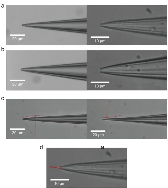
Pull pipettes with resistance between 5–7 MΩ using the pipette puller (Fig. 3). A good starting point is to use patch pipette geometries that have already been proven to work in brain slices, or otherwise empirically optimized. Refer to Box 1 for a description of the ideal pipette geometry that gives optimum autopatching in our laboratory.

A

uthor Man

uscr

ipt

A

uthor Man

uscr

ipt

A

uthor Man

uscr

ipt

A

uthor Man

uscr

ipt

PROCEDURE

1 Autopatcher pipette actuator: Follow the instructions in the assembly manual

in Supplementary Data 3 and install the pipette actuator on an optics table (Fig. 2c). Isolate the optics table from mechanical vibrations and electrical noise (Fig. 2a).

2 Autopatcher control box: Follow the instructions in the assembly manual in

Supplementary Data 4 to assemble and test the autopatcher control box. Assembling the autopatcher control box requires proficiency in electronic and mechanical fabrication. Alternately, a fully assembled control box can be procured from a commercial vendor (e.g., Neuromatic Devices). Connect the pneumatic pressure output on the front panel of the control box to the pipette holder’s pressure input using 3.175 mm (1/8th inch) outer diameter

non-deformable tubing and barbed Luer fittings as necessary. Connect the USB cable from the box to the computer and connect the BNC connections on the front panel to the patch amplifier and traditional external digitizer (Fig. 2b and d).

3 Headplate fabrication: See Supplementary Data 2 and use the ‘Head Plate CAD.sldprt’ file to cut the headplates from 1.59 mm (1/16th _{inch) thick Delrin}

sheet using a laser cutter. Alternately, the fabricated headplates can be

commissioned from commercial fabrication service providers. Use a high speed rotary tool (e.g., Dremel) with a cylindrical sanding attachment to sand the bottom of the headplate to define a curved contour along the headplate window that mates with the curved surface of the mouse skull (Fig. 4a).

4 Head fixation base fabrication: See Supplementary Data 2 and use ‘Head fixation base CAD.sldprt’ to 3D print the head fixation base in acrylonitrile

butadiene styrene (ABS) plastic using a 3D printer. Alternately, the custom head fixation base can be commissioned from a commercial 3D printing vendor. Install the head fixation base on the optics table underneath the autopatcher pipette actuator and clamp securely in position using bolts or table clamps (Fig. 2c).

CRITICAL STEP: Secure clamping is very important. The custom

headplates are surgically attached to the skull with dental cement and are then fastened to this base at the beginning of the experiment. If the base is not secured, then motion from the mouse or other disturbances could cause the skull to move relative to the pipette. This will significantly reduce yield and recording stability.

5 Ground electrode: Take an insulated wire, 300–450 mm long, and solder a

Ag-AgCl pellet on one end and a 1 mm gold coated pin on the other end. Cover soldered sections with insulating heat shrink tubing and shrink it using a heat gun. Plug the gold-coated pin into the back of the amplifier headstage. The Ag-AgCl pellet is kept on top of the skull, submerged in the ACSF bath during the patch experiment using a “helping hand” device (Step 25 in the protocol).

A

uthor Man

uscr

ipt

A

uthor Man

uscr

ipt

A

uthor Man

uscr

ipt

A

uthor Man

uscr

ipt

6 Ag-AgCl pipette electrode wire: Take a 50 mm long silver wire and immerse

25 mm of its length in bleach for 5–10 minutes to make the Ag-AgCl pipette electrode. Clean it thoroughly with filtered deionized water and connect the non-bleached end to the gold pin at the top of the pipette holder. Install the pipette holder with the Ag-AgCl wire in the amplifier headstage.

Software Setup

7 Patch amplifier and data acquisition software: Install the data acquisition

software (e.g., Clampex, Molecular Devices), and the patch amplifier control software (Multiclamp Commander, Molecular Devices). Connect the amplifier and external digitizer directly to the USB ports on the computer. Do not connect them through a USB hub or splitter. In the amplifier control software, configure the feedback resistor to 500 MΩ for both voltage and current clamp. Set the “External Command Sensitivity” to 20 mV/V and 400 pA/V for voltage and current clamp respectively.

8 Autopatcher software installation: First install the LabVIEW programming

environment (National Instruments, LabVIEW 2011 version or later), as the freely available autopatcher code is written in this environment. Also install the latest data acquisition drivers (DAQmx, National Instruments). Next, download and open Supplementary Data 1. This contains all the code necessary to run the autopatcher in LabVIEW. Updates for this software can be found at

www.autopatcher.org. Open the ‘Autopatcher 2000.llb’ file within

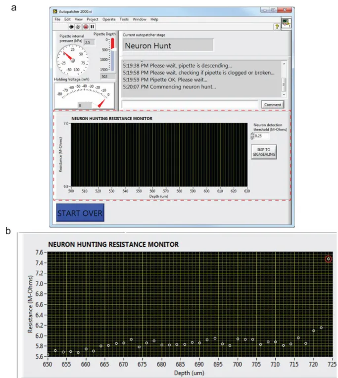
Supplementary Data 1 with LabVIEW to show a list of all the “.vi” files used in the code. Open the ‘Autopatcher 2000.vi’ file within ‘Autopatcher 2000.llb’ and you should see the graphical user interface (GUI) used to control the autopatcher (Fig. 5).

9 Programmable motor software: Install the drivers and software provided by

the manufacturer for controlling the programmable linear motor. If using the TDC001 motor controller from Thorlabs, this is the APT controller software.

10 Configuring Autopatcher Software: Follow the instructions in the

configuration manual ‘Autopatcher software configuration manual.pdf’ in Supplementary Data 1 to configure the autopatcher software to recognize and control the programmable motor, internal digitizer, and amplifier software.

11 Restart the computer: Restart the computer after completing all the software

installations to allow the operating system to register all the changes.

PAUSEPOINT: This completes the setup of the autopatcher hardware and

software. The following steps describe the protocol for performing the in vivo experiment. Prior to this, it is recommended that the experimenter follow the steps described in Supplementary Note 1 to test the autopatcher function using a pipette navigating in a saline bath as a proxy for the intact brain. Beyond this initial setup, it is also important to clean the pipette holder, silver wire, ground wire, pipette storage box, and pipette puller bars with ethanol and filtered

A

uthor Man

uscr

ipt

A

uthor Man

uscr

ipt

A

uthor Man

uscr

ipt

A

uthor Man

uscr

ipt

deionized water at least monthly to reduce clogging from precipitates and dust accumulation.

Surgical preparation: Headplate attachment and craniotomy

12 Anesthetize the mouse: Anesthetize a mouse using an approved anesthesia

protocol. We typically use a cocktail of 100 mg/kg of ketamine and 10 mg/kg of xylazine, or 1–2% isoflurane in oxygen. Maintain the animal’s anesthetic plane throughout surgery and recording by regularly testing the depth of anesthesia and adjusting anesthetic dosing according to the approved animal protocol.

CAUTION: All procedures involving animals must be performed in strict

compliance with institutional and federal regulations concerning laboratory animals. The procedure we describe here was approved by the Division of Comparative Medicine (DCM) at the Massachusetts Institute of Technology.

13 Prepare the mouse for surgery: Apply ophthalmic ointment to the eyes, and

use hair trimmers and scissors to trim hair on top of the head (Fig. 4b) to prepare the scalp for incision. Scrub the head with a sterile cotton swab soaked in betadine, followed by scrubbing with 70% ethanol to clean the scalp (repeat ~3 times as required). Ensure all hair clippings are removed from the surgical area during this procedure.

14 Fix the mouse in stereotaxic apparatus: Fix the mouse in the stereotaxic

apparatus using the ear and mouth bars. Adjust the ear bars and nose cone of the stereotax such that bregma and lambda reference points are at the same height and the midline is parallel to the anterioposterior axis of the stereotax frame. Ensure the mouse is placed on a heating pad with a temperature probe to regulate body temperature during the surgical procedure.

15 Incise the scalp and expose the skull: Using a #10 surgical blade, make a clean

longitudinal incision (anterior to posterior) (Fig. 4c). Use small retractors to pull apart the skin over the skull. Use a micro curette to remove fascia. Identify the location for the craniotomy using the stereotaxic coordinates (Fig. 4d). Using a burr drill bit, gently make a burr hole at the spot to mark the location of the craniotomy. Do not drill all the way through the skull.

16 Implant the skull screws: Using a dental drill, drill three anchor holes (~500

μm diameter) into the skull. Screw in the self-tapping skull screws into the drilled holes (indicated by the three small red dots in Fig. 4e). The location of the skull screws should be made so that the desired recording craniotomy location is roughly centered inside the headplate window. Place two posterior skull screws and one anterior skull screw with approximately 7 mm between the anterior and posterior positions so that when the headplate is fixed the skull screws are just inside the ‘window’ of the headplate.

17 Attach the headplate: Clamp the headplate to the stereotaxic arm so that it is

horizontal in the stereotax frame and then lower the stereotaxic arm until the headplate sits on the exposed skull. Apply freshly mixed dental acrylic cement

A

uthor Man

uscr

ipt

A

uthor Man

uscr

ipt

A

uthor Man

uscr

ipt

A

uthor Man

uscr

ipt

around the skull screws and around the periphery of the headplate (Fig. 4f). Do not apply the acrylic cement over the craniotomy location. This should cure in 10–15 minutes. Picture of the skull surface before and after the headplate attachment is shown in Figure. 4g.

18 Open the craniotomy for recording: Gently mill down the surface of the skull,

in a circular area approximately 1 mm in diameter, until the bone tissue is thin enough to appear flaky and translucent (Fig. 4h and Fig. 4i). Then use a 31-gauge needle to pick away at the desired point on the thinned skull very gently, opening up a single small hole approximately 500 μm in diameter, inducing minimal brain exposure (Fig. 4j and Fig 4k). Keep the brain surface wet with ACSF while attempting to open the craniotomy. Good technique for opening craniotomies has been previously described by Lee et al20. Ensure the craniotomy has been cleared of all bone debris, before proceeding to the next step.

CRITICAL STEP: The size and quality of the craniotomy has a significant

influence on the yield and success rate of autopatching. This has been well documented by other groups performing manual in vivo whole cell patch clamping20.

Make sure that the surface of the brain is not damaged when attempting to dislodge and lift off the bone.

19 Perform a durotomy: Use a 31 gauge needle to cut a 100–500 μm slit in the

dura while keeping the tip of the needle pointing tangentially to the surface of the brain to prevent damaging the brain. Using the needle or fine forceps, slowly fold the dura to either side of the incision to create an opening. Bleeding can be controlled with sterile absorbent pads or by perfusing the craniotomy with ACSF. This step should be done with caution if there are major blood vessels present.

20 Head fix the mouse in the autopatcher: Once surgical preparation is complete,

secure the mouse to the custom head fixing base in the autopatcher (Fig. 2c) by fastening the headplate to the mouse head fixation base using #4–40 socket head screws. Keep the mouse on a heating pad to ensure that the body temperature is regulated throughout the autopatching experiment.

Initializing software programs for autopatching

21 Start the amplifier control software: Open the amplifier software (e.g.,

Multiclamp Commander). The amplifier software should automatically

recognize the amplifier connected to the computer. Set the correct channel of the amplifier to voltage clamp mode.

22 Start the data-acquisition software: Open and run the data acquisition

software (e.g., Clampex, Molecular Devices) to monitor and record the currents measured during the experiment.

A

uthor Man

uscr

ipt

A

uthor Man

uscr

ipt

A

uthor Man

uscr

ipt

A

uthor Man

uscr

ipt

23 Start the autopatcher software: Open the ‘Autopatcher 2000.vi’ in LabVIEW

and click the ‘RUN’ button (see Supplementary Data 1). The autopatcher will initialize the control box and a new LabVIEW program window with the motorized manipulator controls will appear in 30–40s.

24 Start a new trial in the autopatcher software: Set the recording depth at

which you want the autopatcher to start searching for neurons in the ‘Pipette

depth to begin neuron hunting (micrometers)’ numerical entry box and set

the depth at which you want the autopatcher to stop searching for neurons in the

‘Pipette depth to stop neuron hunting (micrometers)’ numerical entry box

(Fig. 5). Click the ‘BEGIN NEW TRIAL’ button. A pop-up dialog box will appear instructing the experimenter to install a new pipette for autopatching. Throughout the operation of the software, Panel 4 of the GUI (see Fig. 4) will change periodically to report the most current information or collect input from the user that is appropriate for the current stage (Supplementary Video 1).

D. Setting up autopatcher for autopatching trial

25 Install ground electrode: Place the ground wire’s Ag/AgCl pellet on top of the

skull close to the craniotomy.

CRITICAL STEP. During operation, ensure that the ground wire Ag/AgCl

pellet is submerged in the ACSF solution above the skull surface and is not subject to any mechanical motion.

26 Inspect the craniotomy: Perfuse the craniotomy with sterile ACSF if needed to

clean the surface (e.g., of any residual blood).

27 Install a pipette in the autopatcher: Fill a patch pipette with internal pipette

solution using a syringe filter and Microfil and install in the pipette holder.

CRITICAL STEP: Always use a fresh, unused pipette for every trial. Do not

attempt to re-use patch pipettes from a previous trial.

To achieve a closed circuit connection, ensure that there is sufficient solution in the pipette to submerge a portion of the Ag-AgCl wire when the pipette is installed in the pipette holder.

Ensure the internal pipette solution is kept on an ice bath for the duration of the experiment and is filtered (0.2 μm pore size) before backfilling the pipette to prevent internal clogging of pipettes. It is recommended to use the pipettes within a few hours of pulling.

28 Set pressure states in the autopatcher control box: Adjust the autopatcher

control box pressures by adjusting the knobs on the control box’s front panel. Set the high positive pressure to 800 mBar, low positive pressure to 25 mBar, low negative pressure to −15 mBar, and high negative pressure to −300 mBar.

29 Position the pipette for autopatching: Carefully position the tip of the patch

pipette 20–30 μm above the brain surface using the manual 3-axis manipulator. The size of the craniotomy, and the pipette, and other known quantities, can

A

uthor Man

uscr

ipt

A

uthor Man

uscr

ipt

A

uthor Man

uscr

ipt

A

uthor Man

uscr

ipt

serve as a “scale bar” for this process. During this procedure, maintain a thin (5– 30 μm) film of fluid over the surface of the brain to prevent the tissue from drying out. Use the stereomicroscope to visualize the pipette tip and craniotomy in this step. Measurements of depth traversed by the autopatcher in subsequent steps are referenced from this starting position. After the tip is positioned, add ACSF until both the tip of the patch pipette and the ground pellet are submerged. This will complete the circuit.

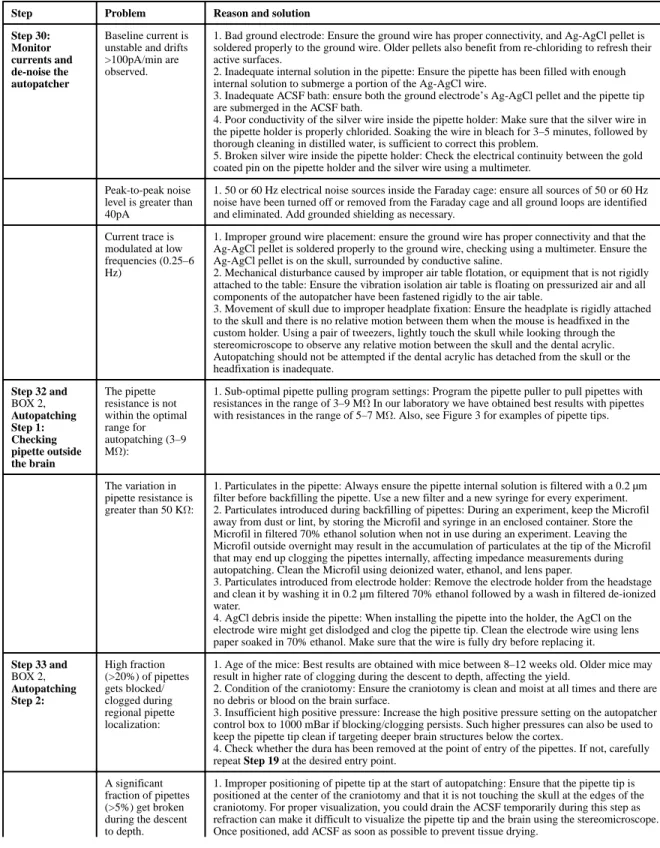
30 Monitor currents and de-noise the autopatcher: Observe the currents being

measured by the amplifier in the data acquisition software. Eliminate any sources of 60 Hz (or 50 Hz depending on geographical region) electrical noise. This can be done by grounding the Faraday cage and the vibration isolation table to the signal ground of the patch amplifier, identifying sources of noise such as microscope lamps and power supplies and either shielding them, powering them down, or relocating them outside the Faraday cage. Shielding the headstage with metal foil and the space surrounding the silver wire may also help. All metal foil shielding should be connected to the optic table ground. The peak-to-peak noise level in the current measurement should be less than 40pA. This completes the manual setup stage of an autopatching trial.

31 Begin an autopatching trial: Click ‘OK’ in the pop-up dialog box in the

autopatcher GUI (referred to in Step 24). The autopatcher will now perform automated whole cell patching until the point when the experimenter choses to either record in whole cell or cell attached mode. These automatically performed steps are described in Box 2 (see also Figures 5–7). Some of these automatic steps may result in outcomes that require user intervention. Steps 32 and 33 describe what to do if such conditions are encountered.

Step 32User intervention if pipette is found to be unsuitable for autopatching (BOX

2, Autopatching Step 1): Click ‘OK’ to stop the autopatcher program. Restart a new trial from Step 24. This step is not required if the autopatcher proceeds to

Autopatching Step 2.

Step 33User intervention if pipette gets clogged, fouled or broken during descent to recording depth (BOX 2, Autopatching Step 2): Click ‘OK’ to stop the

autopatcher program. Restart a new trial from Step 24. This step is not required if the autopatcher proceeds to Autopatching Step 3.

Step 34User inputs during gigasealing (BOX 2, Autopatching Step 5): If a

cell-attached recording is desired, click ‘NEXT’ to proceed to recording and proceed to Step 37. If whole-cell recording is desired, proceed to Step 35.

Step 35Confirming gigaseal formation: Check that a successful gigaseal has been

obtained (BOX 2, Autopatching Step 5.ii). If it has, proceed to step 36. If it has not and you wish to start a new trial, click ‘START OVER’ to stop the current trial and start a new trial from Step 24.

Step 36Break-in: Press the ‘ATTEMPT BREAK IN’ button to break into the

gigasealed neuron. The autopatcher applies a high negative pressure pulse,

A

uthor Man

uscr

ipt

A

uthor Man

uscr

ipt

A

uthor Man

uscr

ipt

A

uthor Man

uscr

ipt

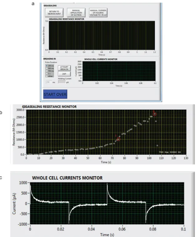
followed by an assessment of the membrane resistance to detect a successful break-in. The holding current required to hold the cell at −65 mV in voltage clamp after each break-in attempt is updated in the ‘Holding Current (pA)’ report boxes. The current trace corresponding to the injection of a 10 mV voltage square wave after a break-in attempt is plotted in the ‘WHOLE CELL

CURRENTS MONITOR’ graph (Fig. 7c). If whole cell patch clamping is not

obtained, proceed to option A. If a whole cell patch clamp recording is obtained proceed to Option B. For a typical mouse cortical pyramidal neuron, successful break-in indicated by a membrane resistance <200 MΩ and current injection required to voltage clamp the patched cell at −65mV of <200 pA which occurs in greater than 80% of successful gigaseals24. A representative screenshot of the current trace plotted in the ‘WHOLE CELL CURRENTS MONITOR’ graph after a successful break-in attempt is shown in Fig. 7c.

Option A) Whole cell patch clamp recording is not obtained.

i. We recommend you attempt the break-in process 1–5 times, with increasing negative pressure pulse duration (250, 500, 750 and 1000 ms durations)

Alternatively, use the ‘ZAP!’ button to attempt break-in, which applies a 250 mV amplitude pulse for 200 ms while applying low suction pressure instead of high suction pulses. If whole cell patch clamp recording is obtained, proceed to option B, otherwise proceed to next step.

ii. If the gigasealed cell is lost during breaking in, or leaky whole cell recording is obtained (indicated, for a typical mouse cortical pyramidal neuron, by a membrane resistance <200 MΩ and current injection required to voltage clamp the patched cell at −65mV of >−200 pA), click ‘START OVER’ to stop the current trial and start a new trial from Step 24.

Option B) Whole cell patch clamp recording is obtained

i. Click the ‘NEXT’ button in the autopatcher software GUI.

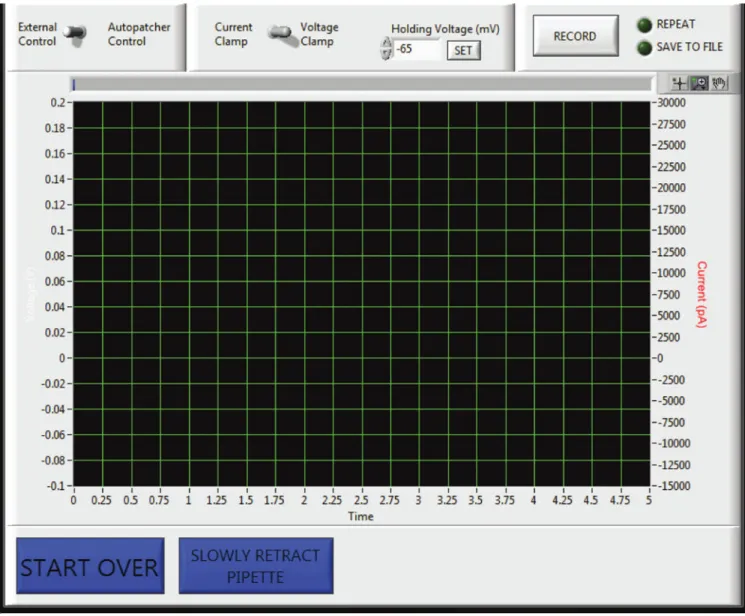
Step 37 Record the whole cell patched neuron: Record in voltage or current

clamp mode using either the autopatcher software or in commercial software; use the ‘External Control’ toggle to switch between these two states if required (Fig. 8). By default the autopatcher holds the whole cell patched cell in voltage clamp mode at −65mV and starts in the ‘External

Control’ state.

38 Assess cell quality: Use the Multiclamp Commander software controls to

perform electrode compensation and access resistance compensation as needed. Use the ‘Membrane test’ function in the data acquisition software (e.g., Clampex) to record the cell parameters such as membrane

capacitance, access resistance, membrane resistance, and holding current. At this stage, pipette series resistance, pipette capacitance, and whole cell capacitance (in the case of a voltage clamp recording) may also be

compensated using the amplifier control software and the ‘Membrane Test’ procedure as described in29. The cell can then be recorded either in voltage

A

uthor Man

uscr

ipt

A

uthor Man

uscr

ipt

A

uthor Man

uscr

ipt

A

uthor Man

uscr

ipt

or current clamp using the data acquisition software. (The recording can also be done entirely in the autopatcher software by switching the left toggle switch in the autopatcher software GUI to ‘Autopatcher Control’ and pressing ‘Record’, Fig. 8). The user can switch between current and voltage clamp by switching the right toggle switch with the ‘Current

Clamp’ and ‘Voltage Clamp’ labels. This will send a command to

Multiclamp Commander to switch modes. The basic recording and stimulation capability of the software can be extended and customized using the LabVIEW programming environment if of interest (but this is beyond the scope of this paper).

39 Pipette retraction for recovering biocytin filled cell: After recording

from the cell, press the ‘SLOWLY RETRACT PIPETTE’ button in the autopatcher software GUI to retract the pipette in steps of 3 μm every 1 second for up to a total distance of 150 μm followed by a fast retraction to the surface of the brain (Fig. 8). The initial slow retraction allows the gradual resealing of the biocytin-filled cell accompanied by formation of an outside-out patch at the pipette tip. This will preserve the morphology for post experiment processing and reconstruction.

TIMING

The reader should budget an initial setup time for installing and integrating all components of the autopatcher. If all components have been procured at the time of setup, assembling the pipette actuator (Step 1) takes 30–60 minutes. The autopatcher control box is the most involved setup step (Step 2), and it should take 2–3 days assuming that all the components were procured and circuit boards pre-fabricated. The custom head fixation base and headplates take ~1 day to fabricate (Steps 3 and 4). Fabricating the ground electrode and preparing the pipette holder takes ~30 minutes (Steps 5 and 6). Once the hardware

components have been set up, installing and configuring the software takes 3–4 hours (Steps

8–11).

Each experiment commences with the surgical preparation of a mouse, which typically takes 45–60 minutes to complete (Steps 12–20). Once the mouse is ready for autopatching, initializing the autopatcher software at the beginning of the experiment takes ~5 minutes (Steps 21–24). Installation of the pipette in the autopatcher and positioning it at the craniotomy typically takes 2–3 minutes (Steps 25–31) while the autopatching itself takes 3– 7 minutes to complete (BOX 2, Autopatching Steps 1–5, Steps 36 and 37). Time duration of recording from each whole cell patched neuron is determined by the specific experimental goals.

TROUBLESHOOTING

See Table 1 for troubleshooting guidance.

A

uthor Man

uscr

ipt

A

uthor Man

uscr

ipt

A

uthor Man

uscr

ipt

A

uthor Man

uscr

ipt

EXPECTED RESULTS

The autopatcher can be used to obtain high quality current and voltage clamp data from anesthetized mice (Fig. 9a–d), and recorded neurons can be filled with biocytin for morphological analysis (Fig. 9e). As described previously, under optimized experimental conditions (as described here), one can expect successful whole cell recordings in ~32.9% of the trials on average (n = 24 out of 73 trials)24, with greater than 60% of the trials yielding good recordings for attempts made within the first hour after opening a fresh craniotomy. Variability in yield might be observed due to variations in the quality of pipettes, the quality of the surgical preparation of the mouse, and the quality of the craniotomy. While the autopatcher has been configured to accept pipettes with resistances between 3–9 MΩ, the generally acceptable range for patch pipette resistances, in our experience best results were obtained using pipettes with resistances between 5–7 MΩ. Patching different neuron types or at different depths or in different species may require different pipette geometries and software settings. The yield of autopatching declines the longer the brain is exposed after the craniotomy is made, as well as with the number of patch attempts made in a particular craniotomy. One strategy to overcome this (if allowed by the experiment) is to attempt autopatching in the more dorsal regions before targeting ventral regions in the pipette descent path. Once cells are autopatched, the cells can be held for an average of ~45 mins with the longest recordings lasting up to three hours, using a quality criterion of resting membrane potential <−50 mV and spike amplitude > 35mV. The throughput of the

autopatcher is governed by the time taken to run each trial (3–7 minutes, including the time taken to install the pipette in the setup) and the desired recording duration, which can vary depending on the experiment. There is ongoing work to combine the autopatcher with technologies that can automatically perform craniotomies29, change pipettes (to enable serial autopatching without human intervention), and potentially to enable parallel computer control of multiple autopatchers with a significant increase in throughput30.

Quality of recordings

The quality of neuronal recordings obtained with the autopatcher is comparable to that obtained via manual whole cell patch clamping by skilled manual in vivo patch clamp practitioners. In our original study24, we compared the autopatched recordings to those obtained via fully manual patch clamping using commonly used metrics: the access resistance, the holding current required to voltage clamp neurons at −65mV, the resting membrane potential and the recording time. In all these comparisons, no significant difference was observed between autopatched neurons and those obtained via standard in vivo patch clamping protocols. These metrics may serve as positive controls for success of the autopatching procedure.

Cell types and morphologies of autopatched neurons

In our original study24, we analyzed the cell types obtained by the autopatcher. Of the neurons recorded in the cortex and hippocampus in a mouse (91% of all cells patched), typically 68% exhibited regular spiking characteristics, 4% exhibited burst firing patterns, 13% exhibited irregular spike characteristics, 4% exhibited spikes followed by smaller

A

uthor Man

uscr

ipt

A

uthor Man

uscr

ipt

A

uthor Man

uscr

ipt

A

uthor Man

uscr

ipt

spikelet events suggestive of backpropagation of action potentials in dendritic recordings, and 2% had spike firing that accelerated. In 9% of the neurons, steady (2s long) current injections over the firing threshold resulted in single action potentials fired, typical of fast adapting neurons. 9% of the recorded cells lacked spiking activity when the membrane potential was depolarized to −30 mV via steadily increasing current injections. Along with this observation and their low cell capacitance characteristics, we concluded that these were glial cells. While not a comprehensive study, these data do illustrate that a variety of cell types can be patch clamped in vivo using the autopatcher.

Including 0.4% biocytin (W/V) in the internal pipette solution while autopatching enabled morphological characterization of the recorded cells via standard immuno-histochemical staining protocols. We developed several optimization strategies to obtain high quality morphological reconstructions of autopatched neurons. These include: configuring the autopatcher pipette actuator at an angle (45° to the vertical axis) so as to minimize the number of “ghost stained” (e.g., stained with background levels of biocytin ejected during the approach of the patch pipette) cells in the brain slice containing the recorded neuron, and shortening the duration of recording (10–15 minutes). In our experiments, we were able to recover the morphologies of approximately 75% of the recorded cells based on intensity of staining as well as staining of fine dendritic arbors- which are absent in the “ghost stained” neurons that are found nearby. Of the cells that were morphologically identified, 70% of neurons autopatched in the cortex were pyramidal cells exhibiting apical dendritic structures (Fig. 9c), similar to observations made in other studies6.

Generalizability of autopatching algorithm

The algorithm used for autopatching was derived in experiments conducted in the cortex of anesthetized mice, but was also useful for obtaining recordings in the hippocampus – exhibiting a degree of generalizability of the algorithm across brain regions. The algorithm is robust enough to allow usage of optic fibers with the patch electrode for simultaneous optogenetic stimulation and autopatching. In a series of experiments, a 200 μm optical fiber was attached to the pipette such that the tip of the fiber was 600 μm lateral from and 500 ± 50 μm above the tip of the electrode tip. This assembly was lowered into the brain using the autopatcher to obtain whole cell patch recordings and subsequently measured photo-evoked hyperpolarization of motor cortex neurons expressing the red-shifted optogenetic silencer Jaws26 (Fig. 9g) and photo-evoked spikes from neurons expressing

channelrhodopsin-2 in a Thy1-ChR2 transgenic mouse31 (Fig. 9h). Coupling of other devices to the autopatcher setup32 may enable the integration of the autopatcher into experiments involving extracellular recording, pharmacological infusion and other

neuroscience strategies of importance. As a final note, the protocol described above has been tried and tested in anesthetized mice. We have also successfully utilized the autopatcher to obtain whole cell patch recordings in awake headfixed animals (Fig. f), both in a fully immobilized setting11, 33 as well as from headfixed animals on a spherical virtual reality treadmill14, 34.

A

uthor Man

uscr

ipt

A

uthor Man

uscr

ipt

A

uthor Man

uscr

ipt

A

uthor Man

uscr

ipt

Supplementary Material

Refer to Web version on PubMed Central for supplementary material.

Acknowledgments

We thank Brian D Allen and Ho-Jun Suk for feedback on the manuscript. CRF acknowledges the NIH BRAIN Initiative (NEI and NIMH 1-U01-MH106027-01), NIH Single Cell Grant 1 R01 EY023173, NSF (EHR 0965945 and CISE 1110947), NIH Computational Neuroscience Training grant (DA032466-02), Georgia Tech Translational Research Institute for Biomedical Engineering & Science (TRIBES) Seed Grant Awards Program, Georgia Tech Fund for Innovation in Research and Education (GT-FIRE), Wallace H. Coulter Translational/Clinical Research Grant Program and support from Georgia Tech through the Institute for Bioengineering and Biosciences Junior Faculty Award, Technology Fee Fund, Invention Studio, and the George W. Woodruff School of Mechanical Engineering. ESB acknowledges NIH 1R01EY023173, the New York Stem Cell Foundation-Robertson Award, NIH Director’s Pioneer Award 1DP1NS087724, NIH Director’s Transformative Award NIH 1R01MH103910, and NIH BRAIN initiative grant NIH 1R24MH106075. GTF acknowledges a Friends of the McGovern Institute Fellowship.

References

1. Bruno RM, Sakmann B. Cortex is driven by weak but synchronously active thalamocortical synapses. Science. 2006; 312:1622–1627. [PubMed: 16778049]

2. Arenz A, Silver RA, Schaefer AT, Margrie TW. The contribution of single synapses to sensory representation in vivo. Science. 2008; 321:977–980. [PubMed: 18703744]

3. Brecht M, Schneider M, Sakmann B, Margrie TW. Whisker movements evoked by stimulation of single pyramidal cells in rat motor cortex. Nature. 2004; 427:704–710. [PubMed: 14973477] 4. Chadderton P, Margrie TW, Hausser M. Integration of quanta in cerebellar granule cells during

sensory processing. Nature. 2004; 428:856–860. [PubMed: 15103377]

5. Eberwine J, et al. Analysis of gene expression in single live neurons. Proc Natl Acad Sci U S A. 1992; 89:3010–3014. [PubMed: 1557406]

6. Rancz EA, et al. Transfection via whole-cell recording in vivo: bridging single-cell physiology, genetics and connectomics. Nat Neurosci. 2011; 14:527–532. [PubMed: 21336272]

7. Margrie TW, Brecht M, Sakmann B. In vivo, low-resistance, whole-cell recordings from neurons in the anaesthetized and awake mammalian brain. Pflugers Arch. 2002; 444:491–498. [PubMed: 12136268]

8. Chadderton P, Agapiou JP, McAlpine D, Margrie TW. The synaptic representation of sound source location in auditory cortex. The Journal of neuroscience : the official journal of the Society for Neuroscience. 2009; 29:14127–14135. [PubMed: 19906961]

9. Chadderton P, Margrie TW, Hausser M. Integration of quanta in cerebellar granule cells during sensory processing. Nature. 2004; 428:856–860. [PubMed: 15103377]

10. Crochet S, Petersen CCH. Correlating whisker behavior with membrane potential in barrel cortex of awake mice. Nat Neurosci. 2006; 9:608–610. [PubMed: 16617340]

11. Crochet S, Poulet JF, Kremer Y, Petersen CC. Synaptic mechanisms underlying sparse coding of active touch. Neuron. 2011; 69:1160–1175. [PubMed: 21435560]

12. Gentet LJ, Avermann M, Matyas F, Staiger JF, Petersen CC. Membrane potential dynamics of GABAergic neurons in the barrel cortex of behaving mice. Neuron. 2010; 65:422–435. [PubMed: 20159454]

13. Gentet LJ, et al. Unique functional properties of somatostatin-expressing GABAergic neurons in mouse barrel cortex. Nat Neurosci. 2012; 15:607–612. [PubMed: 22366760]

14. Harvey CD, Collman F, Dombeck DA, Tank DW. Intracellular dynamics of hippocampal place cells during virtual navigation. Nature. 2009; 461:941–946. [PubMed: 19829374]

15. Hromadka T, DeWeese MR, Zador AM. Sparse representation of sounds in the unanesthetized auditory cortex. Plos Biol. 2008; 6:124–137.

16. Schaefer AT, Margrie TW. Spatiotemporal representations in the olfactory system. Trends Neurosci. 2007; 30:92–100. [PubMed: 17224191]

A

uthor Man

uscr

ipt

A

uthor Man

uscr

ipt

A

uthor Man

uscr

ipt

A

uthor Man

uscr

ipt

17. Kitamura K, Judkewitz B, Kano M, Denk W, Hausser M. Targeted patch-clamp recordings and single-cell electroporation of unlabeled neurons in vivo. Nat Meth. 2008; 5:61–67.

18. Komai S, Denk W, Osten P, Brecht M, Margrie TW. Two-photon targeted patching (TPTP) in vivo. Nat Protoc. 2006; 1:647–652. [PubMed: 17406293]

19. Margrie TW, et al. Targeted whole-cell recordings in the mammalian brain in vivo. Neuron. 2003; 39:911–918. [PubMed: 12971892]

20. Lee AK, Epsztein J, Brecht M. Head-anchored whole-cell recordings in freely moving rats. Nat Protocols. 2009; 4:385–392. [PubMed: 19247288]

21. Lee AK, Manns ID, Sakmann B, Brecht M. Whole-cell recordings in freely moving rats. Neuron. 2006; 51:399–407. [PubMed: 16908406]

22. Lee D, Lin BJ, Lee AK. Hippocampal Place Fields Emerge upon Single-Cell Manipulation of Excitability During Behavior. Science. 2012; 337:849–853. [PubMed: 22904011]

23. Long MA, Jin DZ, Fee MS. Support for a synaptic chain model of neuronal sequence generation. Nature. 2010; 468:394–399. [PubMed: 20972420]

24. Kodandaramaiah SB, Franzesi GT, Chow BY, Boyden ES, Forest CR. Automated whole-cell patch-clamp electrophysiology of neurons in vivo. Nat Meth. 2012; 9:585–587.

25. DeWeese MR. Whole-cell recording in vivo. Curr Protoc Neurosci. 2007:22. Chapter 6, Unit 6. [PubMed: 18428661]

26. Chuong AS, et al. Noninvasive optical inhibition with a red-shifted microbial rhodopsin. Nat Neurosci. 2014; 17:1123–1129. [PubMed: 24997763]

27. Margrie TW, Brecht M, Sakmann B. In vivo, low-resistance, whole-cell recordings from neurons in the anaesthetized and awake mammalian brain. Pflugers Arch. 2002; 444:491–498. [PubMed: 12136268]

28. Schramm AE, Marinazzo D, Gener T, Graham LJ. The Touch and Zap Method for <italic>In Vivo</italic> Whole-Cell Patch Recording of Intrinsic and Visual Responses of Cortical Neurons and Glial Cells. PLoS One. 2014; 9:e97310. [PubMed: 24875855]

29. Pak N, et al. Closed-loop, ultraprecise, automated craniotomies. Journal of neurophysiology. 2015; 113:3943–3953. [PubMed: 25855700]

30. Kodandaramaiah SB, Boyden ES, Forest CR. In vivo robotics: the automation of neuroscience and other intact-system biological fields. Annals of the New York Academy of Sciences. 2013; 1305:63–71. [PubMed: 23841584]

31. Arenkiel BR, et al. In Vivo Light-Induced Activation of Neural Circuitry in Transgenic Mice Expressing Channelrhodopsin-2. Neuron. 2007; 54:205–218. [PubMed: 17442243]

32. Harrison RR, et al. Microchip amplifier for in vitro, in vivo, and automated whole-cell patch-clamp recording. 2014

33. Poulet JFA, Fernandez LMJ, Crochet S, Petersen CCH. Thalamic control of cortical states. Nat Neurosci. 2012; 15:370–372. [PubMed: 22267163]

34. Polack PO, Friedman J, Golshani P. Cellular mechanisms of brain state-dependent gain modulation in visual cortex. Nat Neurosci. 2013; 16:1331–1339. [PubMed: 23872595]

35. Plant, TD.; Eilers, J.; Konnerth, A. Patch-Clamp Applications and Protocols. Boulton, A.; Baker, G.; Walz, W., editors. Vol. 26. Humana Press; 1995. p. 233-258.

A

uthor Man

uscr

ipt

A

uthor Man

uscr

ipt

A

uthor Man

uscr

ipt

A

uthor Man

uscr

ipt

BOX 1

The patch pipette is an important component of the autopatcher and can have significant effect on the yield and quality of recordings obtained by the autopatcher. In our

laboratory, we have consistently obtained high quality and high yield autopatched recordings using pipettes with certain geometrical characteristics. Our pipettes typically exhibit tip diameters of 0.8 – 0.9 μm (corresponding to a range of 5 to 7 MΩresistance, Fig. 3). The general taper of the pipette leading up to the tip has a convex curvature. Pipettes with concave tapers typically have high variability in their resistances and may give variable results while autopatching. Finally, a broad cone angle assists in obtaining stable gigaseals and low access resistance when the whole cell configuration is obtained. To optimize the pipette geometry, a good starting point is to follow the pipette puller’s instruction manual to program it to pull pipettes which have resistances in the range of 3– 9 MΩ. Then the velocity and heat settings (in the case of a Flaming Brown puller) can be adjusted to obtain pipettes of the desired resistance range of 5–7 MΩ. Typically higher velocity and heat settings result in pipettes with longer tapers and smaller tip diameters with corresponding increases in pipette resistance. Refer to the pipette puller’s user manual for instruction on adjusting pulling parameters to obtain pipette with optimum geometries. Further, the performance of the electronics and heating components in the pipette puller can drift over a period of time. To account for these drifts, it is

recommended that the puller is switched on well in advance (or even left on continuously during days of experimentation) so the electronic circuitry is at steady state. Capillary glass with the same dimensions from two different vendors (or even from one batch to the other) can behave very differently when pulled using the same program due to differing melting points and geometrical tolerances. Thus the puller needs to be programmed for each type of glass capillary being used. As a final note, it is important to pull pipettes within a few hours before an autopatching experiment. It is not advisable to use pipettes that have been stored for longer time durations, even if they have been kept in sealed airtight containers, since the surface properties may change due to dust in the air, significantly increasing the chance that the pipette tip will be clogged.

A

uthor Man

uscr

ipt

A

uthor Man

uscr

ipt

A

uthor Man

uscr

ipt

A

uthor Man

uscr

ipt