3-D resistivity forward modeling and inversion using conjugate gradients

3-D resistivity forward modeling and

inversion using conjugate gradients

The MIT Faculty has made this article openly available. Please share

how this access benefits you. Your story matters.

Citation

Zhang, Jie, Randall L. Mackie, and Theodore R. Madden.

“3-D Resistivity Forward Modeling and Inversion Using Conjugate

Gradients.” GEOPHYSICS 60.5 (1995): 1313–1325. © 1995 Society of

Exploration Geophysicists

As Published

http://dx.doi.org/10.1190/1.1443868

Publisher

Society of Exploration Geophysicists

Version

Final published version

Citable link

http://hdl.handle.net/1721.1/108498

Terms of Use

Article is made available in accordance with the publisher's

policy and may be subject to US copyright law. Please refer to the

publisher's site for terms of use.

3-D resistivity forward modeling and inversion

using conjugate gradients

Jie Zhang

*,

Randall L. Mackie

*,

and Theodore R. Madden*

ABSTRACT

We have developed rapid 3-D do resistivity forward modeling and inversion algorithms that use conjugate gradient relaxation techniques. In the forward network modeling calculation, an incomplete Cholesky decom-position for preconditioning and sparse matrix rou-tines combine to produce a fast and efficient algorithm (approximately 2 minutes CPU time on a Sun SPARC-station 2 for 50 x 50 x 20 blocks). The side and bottom boundary conditions are scaled impedance conditions that take into account the local current flow at the boundaries as a result of any configuration of current sources.

For the inversion, conjugate gradient relaxation is used to solve the maximum likelihood inverse equa-tions. Since conjugate gradient techniques only re-quire the results of the sensitivity matrix A or its transpose AT multiplying a vector, we are able to bypass the actual computation of the sensitivity matrix and the inversion of ATA, thus greatly decreasing the time needed to do 3-D inversions.

We demonstrate 3-D resistivity tomographic imag-ing usimag-ing pole-pole resistivity data collected durimag-ing an experiment for a leakage monitoring system near evap-oration ponds at the Mojave Generating Station in Laughlin, Nevada.

INTRODUCTION

The earth is inherently three-dimensional. The interpreta-tion of resistivity data, however, is usually done assuming a 1-D or 2-D geometry, although 3-D interpretation is essential in many applications such as mineral and geothermal explo-ration and environmental surveys for hydrogeologic investi-gations. However, the full use of resistivity techniques in

geophysics has been limited by the inability to accurately calculate anomalies as a result of 3-D features and to efficiently compute an inversion for a large 3-D model. In the recent past, substantial advances have been made in numer-ical modeling techniques for 2-D geologic structures. The techniques for solving a 2-D forward modeling problem include the integral equation method (Hohmann, 1975), the network method (Pelton et al., 1978; Tripp et al., 1984), the finite-element method (Coggon, 1971) and the finite-differ-ence method (Mufti, 1976). Least-squares techniques have been successful in the applications to 2-D inversion prob-lems (Pelton et al., 1978; Tripp et al., 1984; Shima, 1990). However, there are only a few reported studies of 3-D resistivity forward modeling and inversions. Dey and Mor-rison (1979) developed a 3-D forward modeling routine using finite-difference. Petrick et al. (1981) outlined a 3-D alpha-center method that involves solving for image sources rep-resenting conductivity distributions and applying a least-squares algorithm for the inversion. Park and Van (1991) developed a 3-D inversion procedure using maximum likeli-hood inverse theory and Dey and Morrison's (1979) finite-difference forward modeling code. However, their inver-sions were limited to small models because standard matrix inversion techniques were used to solve the maximum likelihood inverse equations. Li and Oldenburg (1994) also used Dey and Morrison's (1979) 3-D finite-difference algo-rithm in an approximate inverse procedure without calculat-ing the 3-D sensitivity matrix and its inversion. They per-formed 1-D linear inversions in the wavenumber domain and obtained an approximate 3-D solution by Fourier transform-ing the 1-D inversion results. Ellis and Oldenburg (1994) presented another approach for solving the pole-pole 3-D resistivity inverse problem which used the conjugate gradi-ent method to minimize a nonlinear objective function and applied the adjoint equation to compute the gradient of the objective function.

In this paper, we use a transmission-network analogy (Madden and Swift, 1969; Swift, 1971) for the 3-D forward Presented at the 64th Annual International Meeting, Society of Exploration Geophysicists. Manuscript received by the Editor May 16, 1994; revised manuscript received December 7, 1994.

*Earth Resources Laboratory, Dept. of Earth, Atmospheric, and Planetary Sciences, Massachusetts Institute of Technology, Cambridge, MA

02142.

© 1995 Society of Exploration Geophysicists. All rights reserved.

1313

1314 Zhang et al.

modeling problem, and we apply conjugate gradient relax-ation to solve both the forward and inverse problems. For the forward problem calculation, conjugate gradient relax-ation is used to obtain an accurate solution of the discretized network equations for dc current flow in the earth. For the inversion, conjugate gradient relaxation is used both for the forward modeling step and for finding a solution to the linearized equations of the maximum likelihood inverse problem. We also recognize that the use of conjugate gradi-ent relaxation in the inversion allows us to bypass the actual computation of the sensitivity matrix. Our fundamental goal is to provide a compact 3-D resistivity code that works quickly and efficiently on a modem computer workstation. Results with both synthetic and real data will be presented. FORWARD MODELING FORMULATION AND BOUNDARY

CONDITIONS

The forward modeling routine will affect both the effi-ciency and accuracy of the 3-D inversion algorithm. There-fore, we explore the details of several different numerical techniques for solving the forward problem and also inves-tigate the effects of the boundary conditions. The equations that govern the dc resistivity response are

Vv(x, y, z) = —p(x, y, z)J(x, y, z), (1)

V • J(x, y, z) = i(x, y, z), (2)

where v(x, y, z) is the electric potential, J(x, y, z) is the current density, i(x, y, z) is the current source distribution, and p(x, y, z) is the 3-D resistivity distribution.

Equations (1) and (2) are seen to be the transmission network equations (Madden and Swift, 1969; Swift, 1971). For a discretized earth, they can be approximated by a network of lumped impedances where the impedances are proportional to the model resistivities. Figure 1 shows a portion of the discretized 3-D resistivity distribution and its

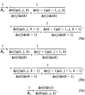
network analog. We define voltage nodes at the top center of each medium block. With this geometry, the impedance elements Rx, Ry, and RZ can be given by

1 1

Rx Ox(i)p(i, j, k) x(i — 1)p(i — 1, j, k) oy(J)&(k) + oy(J)zz(k)

xx(i)p(i, j, k — 1) Ax(i — 1)p(i — 1, j, k — 1)' dy(J)Az(k — 1) tly(j)dz(k — 1)

(3a)

1

Ry Ay(J)p(i, j, k) Dy(J — 1)p(i, j — 1, k)

Ax(i)Oz(k) &x(i)Az(k)

1

+ Dy(j)p(i, _J, k — 1) Dy(j — 1)p(i, j — 1, k — 1)' lix(i)t^z(k — 1) i.x(i)&z(k — 1)

(3b)

1 Ox(i)y(J) RZ &(k)p(i, j, k)

(3c)

where Ox(i), Ay(j), and Az(k) are the grid spacing in each dimension for block (i, j, k), and p(i, j, k) is the resistivity of block (i, j, k). On the right side in Figure 1, a lumped network of 2 x 3 x 2 grids is illustrated, which consists of network nodes, boundary nodes, and impedance branches

between network nodes. Current sources can be placed at

any network nodes, and the voltage is defined at all nodes. Kirchhoff's current law applied to the network results in a linear set of equations that can be written in matrix form as

FIG. 1. A portion of the discretized 3-D resistivity distribution and the resultant lumped network. RX, Ry, and RZ represent network impedances.

Kv=s, (4) where the coefficient matrix K is sparse, symmetric, and positive-definite; v is the voltage vector, and s is the current source vector. For a model with blocks of nx, ny, and nz in three dimensions, the matrix K has a size (nx x ny x nz) by (nx x ny x nz), and v and s have length nx x ny x nz.

Boundary conditions

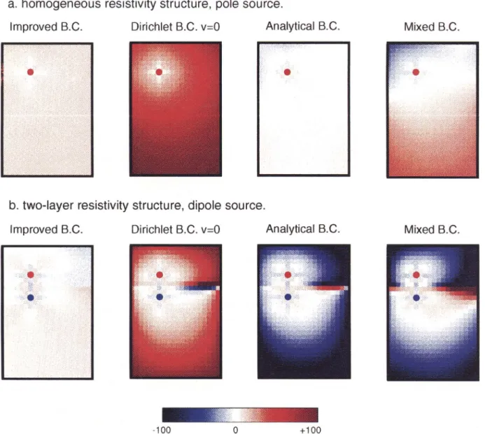
We apply a homogeneous Neumann condition (avlaz = 0) at the earth-air interface and a scaled impedance boundary condition on the sides and bottom that is a modification of Dey and Morrison's (1979) boundary condition. In Figure 2, we illustrate a plan view of the modeling accuracy on the ground surface for four different boundary conditions that we describe below. A single pole or a dipole source with

pole-pole interval 50 m on the surface is assumed. We plot the percentage difference using the formula: 100 X (vQ —

Vnum )Iva, where va is the analytical solution and Vnum is the

numerical solution. Two models are tested: (1) homogeneous half-space (p = 500 ft • m) and (2) two-layer media (pl = 500

fZ • m, P2 = 200 SZ - m, It = 30 m). The models (20 x 30 x 15) are gridded with equal spacing 10 m in all three dimen-sions.

Most of the early work in resistivity modeling used Dirichlet type of boundary conditions, where v = 0 is set at all boundaries except for the free surface (Mufti, 1976; Tripp et al., 1984). Using this boundary condition, one has to establish a large coarse grid system near the boundaries simply for maintaining accuracy in a small central area. Additional computer storage is then required, and the num-ber of grids that can be modeled is limited. The error for an equally gridded model, as shown in Figure 2, can be

tremen-FIG. _{2. Forward modeling accuracy in percentage for four different boundary conditions relative to the analytical solutions: (a)}

pole source, homogeneous resistivity structure, p = 50011 • m; (b) dipole source, two-layer resistivity structure, P1 = 500 0 • m,

h = 30 m, P2 = 200 St • m. Equal grid spacing of 10 m was used in these calculations.

1316 Zhang et al.

dously large because of this boundary condition, and is mostly over 50% on the surface. Another possible boundary condition is to use an analytical solution of the homogeneous medium for the boundary nodes. However, the error for this boundary condition can also be very large if the medium is inhomogeneous and a solution for a homogeneous medium is applied. Consequently, Dey and Morrison (1979) proposed a mixed boundary condition, assuming that the total potential at large distances from the geometrical surface center on the ground has an asymptotic behavior 1/r, giving,

av v

— + - cos 9 = 0, (5)

an r

where 0 is the angle between the radial distance from the geometrical surface center and the outward normal spatial coordinate n on the boundaries. This condition still requires coarse grids near the boundaries, though the accuracy is increased somewhat. However, in solving the inverse prob-lem using conjugate gradient relaxation, we need to be able to compute the forward problem with sources distributed at all the receivers simultaneously and with sources distributed throughout the volume simultaneously (Mackie and Madden, 1993). Therefore, we have modified Dey and Morrison's (1979) boundary condition to account for many sources and exact source locations by considering the local current flow at the boundary nodes as a result of each source. If there are ns sources with sizes I, (i = 1, 2, ... , ns) where the potential at a bottom or side boundary node N is VN (VN = ^k s 1 vp)) and the potential at the next inner boundary node N - 1 is VN_1 (vN-1 = Xks 1 v k^ 1), then we have the following voltage relationship based on Dey and Morrison (1979) because of the ith pole source,

(_) =

(_) (

-

dz c

os 91

vN vN-1 1 i = 1, 2, ... ns, (6)

r;

)

where r1 is the distance between the boundary node and the source i, O is the angle between the radial distance from the source i and the outward normal spatial coordinate n on the boundaries, Oz is the grid spacing at the bottom boundary and should be replaced by Ax or Dy if the side boundaries are considered. For a homogeneous medium, equation (6) gives an exact boundary relation for one current source if r; starts from the location of source i rather than the surface center. We make an assumption that the v/I ratio (voltage/ source current) normalized by the distance r is constant for

each source:

r1 vN- 1 r2 vN_ 1 • rns vN_)1

=p. (7)

11 I2 Ins

Relationship (7) is exact for a homogeneous medium, and gives an approximation for an inhomogeneous medium. If all the sources are included simultaneously, then by linearity the constant p can be written as

VN-1 P = (8) ns k=1 ( Ik rk)

We recognize that the component of the voltage at the node N - 1 caused by the ith source from equations (7) and (8) is therefore given by

i VN-1

vN 1 = (9)

\Ii/ k=1 \rk/

Substituting this into equation (6) and using VN = _ks 1 v ,k)

and VN_1 = Ek = 1 v 1 leads to the boundary condition that we will apply to a general receiver-source problem,

ns

cos 9

1 VN=VN-1 1-Oz 2 L (10) i = 1 r/ ns Ii k=1 ( Ik rk)

To implement the boundary condition [equation (10)] in the network system, we simply scale the near-boundary imped-ance to control the current across the boundary nodes by the following factor,

ns

cos O

(11)

i = 1 ri ns Ik

Il k l rk

As shown in Figure 2, for a pole or dipole source, the modified boundary condition [equation (10)] gives small errors everywhere on the surface for homogeneous or two-layer model while the mixed boundary condition in Dey and Morrison (1979) produces a small error only in the central area. For the dipole case, it also shows relatively large errors in the area at equal or nearly equal distances to both poles. This is because the voltage in this area is small, and the error in percentage is therefore quite sensitive and large when the boundary condition is not properly imposed.

Forward modeling solution

In this study, we apply two different techniques to solve the forward matrix problem, equation (4), i.e., the Greenfield algorithm (Swift, 1971) and the conjugate gradient technique (Hestenes and Stiefel, 1952). The Greenfield algorithm is essentially an efficient algorithm for block tridiagonal matri-ces (Golub and Van Loan, 1990). This algorithm redumatri-ces a large matrix problem into many small submatrix problems. In our implementation of the Greenfield algorithm, the submatrix has a dimension of nx x nz. Although the Greenfield algorithm is slower than the conjugate gradient approach, it gives the exact solution of the difference equa-tions whereas the conjugate gradient method gives only an approximate solution. Thus, the Greenfield algorithm is

useful for the purpose of checking the modeling accuracy

because of boundary conditions and the use of the conjugate gradient method. The numerical calculation shown in Figure 2 used the Greenfield algorithm.

When using the conjugate gradient approach, we need to store only the nonzero elements in the upper triangular part of the symmetric K matrix. In the 3-D forward problem, the number of nonzero elements is 7(nx x ny x nz) - 2 x nx

300 V 0 U 200 E I-100

x ny - 2 x ny x nz - 2 x nx x nz, but we need to store only 4(nx x ny x nz) - nx x ny - ny x nz - nx x nz (diagonal + upper triangular) because of symmetry. To represent the sparse matrix K, we use the row-indexed sparse storage mode (Press et al., 1992), which requires storage of only about two times the number of nonzero matrix elements. Other methods can require as much as three to five times. Efficient algorithms are used to compute K multiplying a vector, which is the essential calculation required in the conjugate gradient techniques.

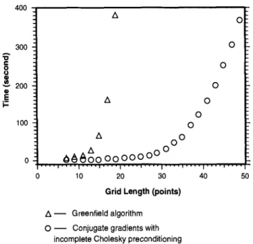
We have also developed efficient algorithms for doing incomplete Cholesky preconditioning that take into account the sparsity of the K matrix. Numerical and theoretical studies indicate that the conjugate gradient techniques work best on matrices that are either well conditioned or just have only a few distinct eigenvalues (Golub and Van Loan, 1990). For linear systems of equations, one can precondition the system using methods such as incomplete Cholesky decom-position (Kershaw, 1978; Papadrakakis and Dracopoulos, 1991), incomplete block decomposition, domain decomposi-tion, or polynomial preconditioners [for general review, see Axelsson (1985)]. For the 3-D resistivity problem, we use the incomplete Cholesky factorization based on rejection by position, forcing the preconditioning matrix to have the same sparsity as the forward modeling matrix. Figure 3 shows a comparison of the computation speed for doing one forward modeling problem using the conjugate gradient relaxation with the incomplete Cholesky preconditioning (open circle) versus the Greenfield algorithm (triangle). The grid length refers to the number of grids in each dimension for a cube

400 0 0 0 0 0 0 0 o

0

•

A®490

O°

°°°

10 20 30 40 50

Grid Length (points)

A — Greenfield algorithm 0 — Conjugate gradients with

incomplete Cholesky preconditioning

FIG. 3. Computation speed comparison for one forward modeling run using the conjugate *radient techniques with incomplete Cholesky preconditioning (open circle) versus the Greenfield algorithm (triangle). The grid length refers to the number of grids in each dimension for cube models. These calculations were conducted on a Sun SPARCstation 2.

model. These tests were conducted on a Sun SPARCstation 2. We used an accuracy criterion of IOv/v < le for these tests. The medium resistivities were completely inhomoge-neous and were defined by the function, p(i, j, k) = 100 x i + 10 x j + 1 x k, so that the speed estimates using the conjugate gradients should represent a lower bound.

MAXIMUM LIKELIHOOD INVERSE PROCEDURE

We apply the maximum likelihood inverse theory devel-oped by Tarantola and Valette (1982) to our 3-D resistivity inversions. In general, geophysical inverse problems are nonunique. The maximum likelihood inverse is one method to obtain a solution to a nonunique inverse problem. This method provides the best fit to the data relative to the a priori information. The mathematical form of the maximum likeli-hood inverse that we use is from Mackie et al. (1988) and Madden (1990), and it closely follows the work of Tarantola and Valette (1982) and Tarantola (1987):

(AkRdd4k + R, )Omk = A/Rdd(d - G(mk))

+ Rmm(m0 - mk) (12)

where,

A = sensitivity matrix d = observed data vector m = model vector

G = forward modeling operator Rdd = data covariance matrix 'mm = model covariance matrix

mo = a priori model

Lmk = model changes for inversion iteration k.

For one source, m receivers and n resistivity blocks, the sensitivity matrix A is defined by Al = aQi/app; i = 1, 2, ... , m; j = 1, 2, ... , n, where Q, is the measurement at the ith receiver and p is the intrinsic resistivity in the jth model block. For a 3-D problem with many sources, how-ever, the matrix A can be very large and have a size equal to (# of sources) x (# of receivers) x (# of medium blocks). Nevertheless, using conjugate gradient relaxation tech-niques to solve the maximum likelihood equations allows us to bypass the actual computation of the sensitivity matrix A, or the inversion of the ATA term. Indeed, we only need the

results of matrix A multiplying an arbitrary vector x and AT

multiplying an arbitrary vector y. As shown in the algorithm given in the Appendix, these vectors are related to the model residuals or the search directions in the conjugate gradient relaxation and are updated at each relaxation iteration.

For the 3-D magnetotelluric (MT) inversion problem, Mackie and Madden (1993) showed that A multiplying a vector could be computed with one forward modeling run with scaled sources distributed throughout the volume. Likewise, they showed that AT multiplying a vector could be

computed with another forward modeling run except with scaled sources at the surface. Thus, for each relaxation iteration, only two forward problems are required to com-pute an update of Omk. The total number of forward

problems per inversion iteration is determined by the num-ber of relaxation iterations carried out at each inversion iteration. Thus, each inversion iteration required only

1318 Zhang et al. 2 x nrel forward problems, which could be substantially

less than doing inversion by traditional methods.

We recognize that we can also compute A and AT multi-plying arbitrary vectors without forming A by using another approach based on rdciprocity (Rodi, 1976). There may be situations where this approach may require fewer forward problems than the method in Mackie and Madden (1993). This will be detailed shortly.

To thoroughly investigate each method (Mackie and Madden, 1993; Rodi, 1976), we present two equations for calculating Ax and ATy that explicitly contain the forward problems required by both Rodi (1976) and Mackie and Madden (1993). In our implementation of the maximum likelihood inverse, we use logarithmic parameterization of the data and model parameters. In all the following equa-tions, however, we keep the sensitivity terms in the original definition, so that the physical meaning can be easily under-stood. To better illustrate the methods, the following algo-rithm is developed for a 3-D problem with one source, m receivers and n resistivity blocks. Problems with more sources can be easily modified.

A potential measurement Q, can be defined as

Q; = at

v,

(13)

where, i = 1, 2, ... , m is the receiver index, v is the voltage vector containing voltage values at all network nodes and for a1T = (0, ... , 0, 1, 0, ... , 0), 1 is the ith

component in the vector a,T, which corresponds to the receiver site i.

The partial derivative with respect to p (medium resistiv-ity) of equation (4) is given by

aK av

— v+K —=0. (14)

ap ap

Substituting equation (13) into (14), we get the sensitivity term,

a

a

pt = –aTK 1

ilK

v. (15)

The matrix Alap contains only a few terms, which are those associated with the medium p in the forward matrix, and it can be analytically derived. The sensitivity matrix A multiplying a vector x has the form

aQ1 aQl aQl

X1 +—X2 + • • • + —xn

aPl iP2 aPn

aQ2 aQ2 aQ2

Ax = - x1 aPl + iP2 x2 + .. + aPn xn

iQm aQm iQm xl + x2+•••+ xn

aPi iP2 aPn

aT₁

az 1( aK aK aK

_ — K xl —v+x2 —v+ +xn —v

1

.

" ap1 ip2 apn

am_m

(16) Similarly, the transposed sensitivity matrix multiplying a vector y is given by,

aK apl v

aK — v

A

Ty = –(Ylai +Y2a2 + ... +Ymam)K 1 ape

aK

—v

aPn

(17) Note that the matrix iK/ap; in these equations contains only a few nonzero terms with algebraic expressions and can be calculated exactly. There are two possible ways to compute Ax and ATy in equations (16) and (17). First, one

can define a vector u for computing equation (16) such that,

1(

= aK aK aK

uK- xl —v+x2 —v+ ...+x v /),

api iP2 aPn

(18) and another vector s for computing equation (17) such that

sT = (_{Ylal +Y2a2 + ... +Ymam)K}-1. (19)

Equation (18) can then be rewritten as

( aK aK aK

Ku= xl —v +x2 —v+•• +xn —v

apt iP2 aPn

(20) To calculate u, we simply do one forward problem with a source vector (xi aK/ap1 V + X2 iK/ap2 V + ••• +

xn aK/ap„ v), in which xl (i = 1, 2, ... , n) is the ith element of the given vector x. The source vector represents the sources distributed throughout the model volume. Like-wise, because K is symmetric, equation (19) can be rewritten as

Ks = (Ylai +Y2a2 + ... +Yoram)• (21)

The term (ylal + y2a2 + • • • + ymam) represents sources distributed at all receiver sites with source size y at receiver i. By doing one forward problem according to equation (21), we can obtain the results of ATy• In these two forward problem equations (20) and (21), however, the source sizes are scaled by the vector components of x and y. As mentioned earlier, these vectors need to be updated after each relaxation iteration. Therefore, the total number of

.

_C 0 C) C) H C) E I-100 90 80 70 60 50 40 30 20 10 b) 200 __ 150_'o C 0 C) 100 C)

E_

I- 50 forward problems per inversion iteration by this method is

2 x nrel.

The second approach is to solve uT = a,TK-1, i = 1,

2, ... , m, which because of symmetry is equivalent to solving Ku = a,, i = 1, 2, ... ,

m

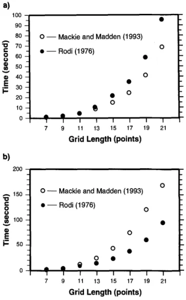
(Rodi, 1976). These are needed by both equations (16) and (17). This suggests that we need to do m (# of receivers) forward problems with a unit source at one receiver site each time. This idea is similar to Rodi's (1976) algorithm for setting up a sensitivity matrix for the MT problem. However, we bypass dealing with each sensitivity term and directly compute the results of the sensitivity matrix or its transpose multiplying a vector as needed in the conjugate gradient relaxation techniques. Once these calculations are done, then each relaxation iteration requires only updating the appropriate vectors, so no further forward problems are necessary. In essence, since the resistivity problem involves point current sources, we see that by doing forward problems with a current source at each receiver, we have effectively generated the numerical Green's functions.

For each inversion iteration, therefore, we see that when using Mackie and Madden's method (1993) 2 + 2 x nrel forward problems are required including two forward prob-lems needed to update the b vector before the start of the relaxation loop (nrel is the number of relaxation steps in one inversion iteration): Using the approach based on Rodi (1976), one would need to do 1 +

m

forward problems per inversion iteration

(m is

the number of receivers). The difference of total computation time between the two meth-ods mostly depends on the number of forward problems required in the inversion procedure. Figure 4 illustrates the difference between the two approaches. For example, with one source and 12 receivers in the field, and three relaxation steps per inversion iteration, this means, by Rodi (1976), 1 + 12 = 13 forward problems for one inversion iteration; by Mackie and Madden (1993), 2 + 2 x 3 = 8 forward problems for one inversion iteration.

However, if we want to take 10 relaxation steps in one inversion iteration for solving the same problem, by Rodi (1976), 1 + 12 = 13 forward problems for one inversion iteration; by Mackie and Madden (1993), 2 + 2 x 10 = 22 forward problems for one inversion iteration.

There is yet an additional way to compute the sensitivity terms. For a network formulation, we can use the Cohn's sensitivity theorem (Tripp et al., 1984), which is efficient when reciprocity is applied. Tripp et al. (1984) solved the 2-D resistivity inverse problem using this approach to explicitly construct the sensitivity matrix. However, Cohn's sensitiv-ity theorem deals with the local current across each network node, so there is a lot of overhead associated with keeping track of the current values across each node. Nevertheless, we have implemented Cohn's sensitivity theorem to provide a cross-check on the other computations.

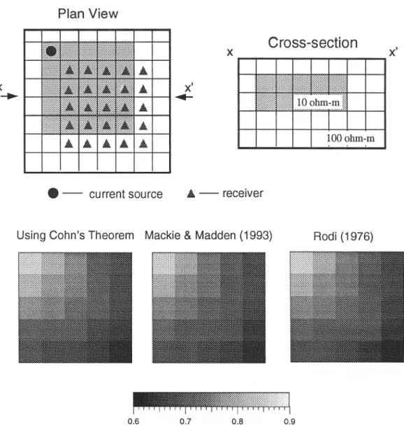
Figure 5 shows the results of the sensitivity matrix multi-plying a unit vector by using three different methods: Cohn's sensitivity theorem (Tripp et al., 1984), the method based on Rodi (1976), and Mackie and Madden's (1993) method. The sensitivity matrix multiplying an unit vector gives the sum-mation of the partial derivatives of each receiver with respect to all medium parameters. This can be understood from equation (16). Clearly, the results from all three

meth-ods are quite comparable to one another, and the differences are minor. The results from Mackie and Madden's (1993) approach and the approach based on Rodi (1976) are almost identical.

Results for synthetic data

Three-dimensional resistivity inversion is very nonunique because there are so many model parameters compared to data points. It is necessary, therefore, to provide constraints to the inversion. Constraints can be applied through the inverse of the model covariance matrix, Rm,;. This matrix is generated prior to the inversion and can be used to weight various model parameters. The model can be smoothed by using off-diagonal terms that couple adjacent parameters. Likewise, the model covariance can be used to correlate model parameters in some predetermined manner, to force certain parameters to have more/less freedom to change

a)

•

0— Mackie and Madden (1993)

• — Rodi (1976)

_•

0 0

•

•

• O 0

• e

11 13 15 17 19 21

Grid Length (points)

0 0— Mackie and Madden (1993) •• — Rodi (1976)

•

O

•

O • 0 • 11 13 15 17 19 21

Grid Length (points)

FIG. 4. Comparison of computation speed for one inversion

iteration with different relaxation steps by using Mackie and Madden's (1993) method and another approach based on Rodi (1976). The grid length refers to the number of grids in each dimension for cube models. These calculations were conducted on a Sun SPARCstation 2.

1320 Zhang at al. during the inversion, or to apply a filter other than

near-neighbor smoothing. In our inversion, we also add a variable damping term to the left-hand side of equation (12) to stabilize the inversion in the beginning, and we tie it to the error in the right-hand side so that as the error decreases, so does the added damping. The damping term a is a X _(1/.:r)

x (right-hand side error), where a is an empirical scaling parameter usually on the order 0.1 to 1.0, and the right-hand side is defined as,

nmod

b(i)b(i) 1 = 1

x 100, (22)

nmod

where b(i) is the right-hand side vector in equation (12). The damping term reduces the influence of the small eigenvalues in the early stages of the inversion, then allows them to

become more influential at the latter stages. In other words, the use of this damping term maintains a stable convergence rate in the maximum likelihood inverse procedure.

Our numerical simulations have shown an unfortunate result of the nonuniqueness of the resistivity problem and the large sensitivity of the near-electrode model blocks that can duplicate the effects of substantial changes deeper in the model. That is, without additional constraints the inversion tends to make large model resistivity changes in the near-surface layers, and especially in the near-electrode model blocks. This is understandable because a check of the sensitivity terms reveals that the near-electrode model blocks normally have the largest sensitivity. After testing many different inversion constraints, we have settled on the following steps as a reasonable approach: (1) we set the starting resistivity of the shallow layers to an average value determined by the nearest source-receiver combinations, (2)

FIG. 5. Results of sensitivity matrix multiplying a unit vector (in natural logarithm) by using three different approaches, Cohn's

sensitivity theorem, Mackie and Madden's (1993) approach, and another approach based on Rodi (1976). The model contains a low resistivity zone.

the model covariance is adjusted so that the upper several layers are weighted less than the bottom layers (this means that initially large resistivity changes are not allowed in the shallow structure), and (3) near-neighbor smoothing is also applied. With these constraints, about 10-15 inversion iter-ations are required to fit the data; however, we obtain much more realistic results than inversions without these con-straints.

To demonstrate our 3-D resistivity inversion, we show the results for a pole-pole array with a grid of 5 x 5 electrodes on the surface and five electrodes in a borehole at one corner (see Figure 6a). The model contains a conductive zone with a resistivity value of 10.0 (fl • m) at a depth of 50 m in the background of 100.0 (l • m). The model size is 50 x 50 x 20 with an equal spacing of 6.25 m in all three dimensions. In this numerical experiment, each electrode is used as a transmitter and also as a receiver. Each time one pole transmits current, voltage measurements are taken at all the

other poles. Therefore, there are 870 readings that are taken as the data input in the inversion. Figure 6b shows the anomaly sensitivity in percentage for two different sources (circled in Figure 6a): one in borehole, the other on surface. To understand numerical modeling accuracy, noise-free syn-thetic data are applied.

To calculate synthetic data for M poles, one needs to do M forward problems with a source at each pole. Therefore, we can modify equations (16) and (17) to include M equations in a column or a row for the Ax and ATy calculations, where x = (x1, x2, ... x,,) and _{Y = (y l),} YJ1) ...

yD),

YJ2), Y z) ...y

2)

,

...

Yu), ...yl

(M)

1)_{). The vector} x still has a dimension of n (the number of model parame-ters), but the vector y now has a dimension of M(M — 1). Therefore, the Ax and ATy calculations become Ax = (fl,

fM)T and ATy = (gl + g2 + • • • + gM), where f, and g1 (i = 1, 2, ... , M) are given by equations (16) and (17), respectively.

FIG. 6. (a) Cross-section (left) and plan view (right) of the test model. Pole-pole geometry is applied for the numerical test; (b) data sensitivity in percentage because of the conductive zone: one source in borehole (left), the other on surface (right) (circled in Figure 6a).

1322 Zhang et al. For a pole-pole problem, since each pole is used both as a

receiver and a transmitter and since reciprocity is automat-ically applied in the field, the results of a,TK-1 as required in equations (16) and (17) are actually obtained in the initial forward modeling step. Therefore, for this pole-pole prob-lem, we prefer the inversion approach based on Rodi (1976), since no additional forward problems are required for doing the inversion after the initial forward modeling step is completed. For a model size of 50 x 50 x 20 (nx, ny, nz) with 30 poles (870 data readings), one inversion iteration with 10 relaxation steps takes 65 minutes (CPU time) on a Sun SPARCstation 2, and 24 minutes (CPU time) on a DEC alpha workstation.

The conductive zone in Figure 6 comprises 16 x 16 x 5 blocks. For this conductive zone, the largest voltage changes on the surface are about 10%. The lateral changes on the surface are smooth, though some rapid changes occur near the anomaly in the subsurface. This simply suggests that we are not able to resolve the sharp features in the subsurface with any number of receivers on the surface. However, if the receiver spacing is too large, spatial aliasing may become a problem. For this test, we used a grid of 5 x 5 surface poles with a pole-pole spacing of 50 m, or 8 grids.

As mentioned earlier, a nonuniform weighting of the model covariance is important to the success of resistivity inversion. For this problem, we use a spatial weighting matrix that contains layer weights varying from le -3 to le -5 for the shallow structures of the a priori model, and le-3 for the deep layers, except near the poles in the borehole a larger weighting of 1e 3 is uniformly applied. The starting model was homogeneous, with a resistivity value of 89.5 fl • m, which is the average apparent resistivity from the closest pole-pole measurements. This gave an initial 93% rms data fit error. After 10 iterations, the data error was reduced to 2.0%. We stop here for this noise-free synthetic test, be-cause the error in the forward modeling is probably about 2.0 to 3.0%. The results are shown in Figure 7. Clearly, the

sharp features of the conductive anomaly, such as the corners, cannot be resolved, however, the location, the average size, and the low-resistivity of the zone can be determined from the inversion.

Analysis of field data

At the Mojave Generating Station in Laughlin, Nevada, a resistivity monitoring system was installed beneath and around one of the evaporation ponds operated by Southern California Edison (Van, 1990; Van et al., 1991). This system uses an 8 x 8 grid of electrodes, with an approximate spacing of 90 m between electrodes. The purpose of this monitoring system is to detect changes in resistivity that would be associated with a leak of saline water from the pond. A sketch map from Van (1990) is given in Figure 8 to show the field layout.

A field test using a scaled down version of the resistivity monitoring system to collect pole-pole data was performed to demonstrate the effectiveness of using this system to detect changes in resistivity associated with the influx of water into the subsurface. The test consisted of a grid of 5 x 5 electrodes that had exactly the same distance scale and surface pole-pole geometry as shown in Figure 6. A back-ground resistivity survey performed prior to the placement

FIG. 7. Inversion results using 25 surface pole-pole data and

5 borehole pole-pole data.

FIG. 8. Map of the field experiment at the Mojave Generating

Station in Laughlin, Nevada (from Van, 1990). A grid of 5 x 5 poles using the same surface geometry shown in Figure 6a was used to collect data, no borehole data available in this case.

of water was used as a comparison for the measurements taken afterwards and to determine the resistivity structure of the test area. Park and Van (1991) applied a 3-D inversion algorithm to image the background resistivity structure. However, as a result of the limitation in the algorithm, they could invert only a small number of model parameters (7 x 7 x 5). In this paper, we present the results of modeling the same data but with more efficient forward modeling and inversion techniques and a mesh of 50 x 50 x 20 grids. Another study using the same techniques to model the resistivity monitoring data collected during the experiment is currently being conducted and will be published separately.

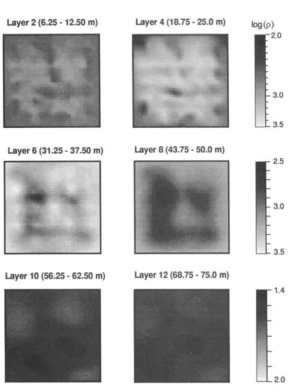
Based on pole-pole apparent resistivity analyses, we find that the resistivities in the shallow structures may vary between 40012. - m and 600 fl - m. Considering the fact that the apparent resistivities decrease with the increase of pole-pole distance and the water table is at the depth of about 45 m (Park and Van, 1991), we believe this estimate is just a lower bound for the average values from the surface down to 30 or 40 m. The rms data fit error for the inversion starts at 76.0% and drops down to 4.2% after 12 iterations, where we stop the inversion. This is because that analysis of the raw data suggests that 85% of the data satisfies reciproc-ity with error below 4%. As shown in Figure 9, from the

FIG. 9. Six layers of the tomographic imaging results for the baseline survey data collected in Laughlin, Nevada (in logarithm

of base 10).

1324 Zhang at al.

surface down to 25 m, no significant lateral changes are resolved, but changes do occur vertically. In layer 2 (6.25 to 12.50 m), the resistivities vary between 600 and 80011 • m. In layer 4 (18.75 to 25.00 m), however, resistivities vary be-tween 1000 and 2000 fl • m. The 3-D variations in the medium become apparent below the depth of 30 m. Between layer 6 and 8, one can see that there is a high resistivity zone (about 2300 SZ • m) near the center. Because the measure-ments have low sensitivity to the medium near the bound-aries at this depth and the a priori model had high resistivi-ties for these layers, the inversion results show a pattern of high resistivity near the boundaries. This is just an artifact rather than true image. The depth of the water table remains the same as what was given in the a priori model, but also shows slight variations with a 3-D pattern. We have run many inversions with different deep resistivity structures in the a priori model each time, and we are always able to resolve the same features.

The average resistivity in each layer shown in Figure 9 is comparable to that obtained by Park and Van (1991). How-ever, our results more clearly show the lateral and vertical variations that are important for studying leakage monitoring data collected afterwards.

SUMMARY

We have developed rapid 3-D dc resistivity modeling and inversion algorithms using conjugate gradient relaxation methods. We have also modified Dey and Morrison's (1979) mixed boundary condition so that it gives more accurate modeling results. Instead of using only one inversion ap-proach, we have tried to obtain a more thorough understand-ing of various techniques, and we have analyzed the advan-tages and disadvanadvan-tages of each technique for the 3-D problem. The inversion algorithms are presented in a general form, which allows us to use pole-pole data and/or dipole data on the surface and/or in boreholes. We have suggested constraints for minimizing the nonuniqueness of 3-D resis-tivity inversions based on an appropriate weighting of the model covariance. However, this procedure by no means guarantees a unique solution or a "true" solution. One must combine the results of other geophysical and geological studies to make the interpretation whenever possible.

We believe that the investigation of subsurface features using 3-D resistivity imaging techniques will become an increasingly important exploration tool in the future.

ACKNOWLEDGMENTS

We would like to thank Prof. Stephen K. Park for his many helpful suggestions and for supplying us with the field data used in this study. Prof. M. Nafi Toksoz, Prof. Dale Morgan and Prof. Stephen K. Park reviewed the manuscript and made many useful comments. Reviews from Prof. Roy J. Greenfield and Prof. Robert G. Ellis helped improve the manuscript. This work was supported by the EPA under grant #CR-821516 to the Massachusetts Institute of Tech-nology.

REFERENCES

Axelsson, 0., 1985, A survey of preconditioned iterative methods for linear systems of equations: BIT 25, 166-187.

Coggon, J. H., 1971, Electromagnetic and electrical modeling by the finite-element method: Geophysics, 36, 132-155.

Dey, A., and Morrison, H. F., 1979, Resistivity modeling for arbitrarily shaped three-dimensional structures: Geophysics, 44, 753-780.

Ellis, R. G., and Oldenburg, S. W., 1994, The pole-pole 3-D DC-resistivity inverse problem: a conjugate-gradient approach: Geophys. J. Int., 119, 187-194.

Golub, G. H., and Van Loan, C. F., 1990, Matrix computation: Johns Hopkins University Press.

Hestenes, M. R., and Stiefel, E., 1952, Methods of conjugate gradients for solving linear systems: J. Res. Natl. Bureau Stand., 49, 409-436.

Hohmann, G. W., 1975, Three-dimensional induced polarization and electromagnetic modeling: Geophysics, 40, 309-324. Kershaw, D. S., 1978, The incomplete Cholesky-conjugate gradient

method for the iterative solution of systems of linear equations: J. Comput. Phys., 26, 43-65.

Li, Y., and Oldenburg, D. W., 1994, Inversion of 3-D DC resistivity data using an approximate inverse mapping: Geophys. J. Int., 116, 527-537.

Mackie, R. L., Bennett, B. R., and Madden, T. R., 1988, Long-period magnetotelluric measurements near the central California coast: A land-locked view of the conductivity structure under the Pacific Ocean: Geophys. J., 95, 181-194.

Mackie, R. L., and Madden, T. R., 1993, Three-dimensional mag-netotelluric inversion using conjugate gradients: Geophys. J. Int., 115, 215-229.

Madden, T. R., and Swift, C. M., Jr., 1969, Magnetotelluric studies of the electrical conductivity structure of the crust and upper mantle, in the earth's crust and upper mantle (edited by Hart, P. J.): Geophys. Mono. 13, Am. Geophys. Union, 469-479. Madden, T. R., 1990, Inversion of low-frequency electromagnetic

data, in oceanographic and geophysical tomography: Elsevier Science Publ., 337-408.

Mufti, I., 1976, Finite-difference resistivity modeling for arbitrarily shaped two-dimensional structures: Geophysics, 41, 62-78. Park, S. K., and Van, G. P., 1991, Inversion of pole-pole data for

3-D resistivity structure beneath arrays of electrodes: Geophys-ics, 56, 951-960.

Papadrakakis, M., and Dracopoulos, M. C., 1991, Improving the efficiency of incomplete Choleski preconditionings: Comm. App. Numer. Methods, 7, 603-612.

Pelton, W. H., Rijo, L., Swift, C. M., Jr., 1978, Inversion of two-dimensional resistivity and induced-polarization data: Geo-physics, 43, 788-803.

Petrick, W. R., Sill, W. R., and Ward, S. H., 1981, Three-dimensional resistivity inversion using alpha centers: Geophysics, 46, 1148-1162.

Press, W. H., Teukolsky, S. A., Vetterling, W. T., and Flannery, B. P., 1992, Numerical recipes: Cambridge Univ. Press. Rodi, W. L., 1976, A technique for improving the accuracy of

finite-element solutions for magnetotelluric data: Geophys. J. Roy. Astr. Soc., 44, 483-506.

Shima, H., 1990, Two-dimensional automatic resistivity inversion technique using alpha centers: Geophysics, 55, 682-694. Swift, C. M., Jr., 1971, Theoretical magnetotelluric and Turam

response from two-dimensional inhomogeneities: Geophysics, 36, 38-52.

Tarantola, A., 1987, Inverse problem theory: Method for data fitting and model parameter estimation: Elsevier Science Publ. Tarantola, A., and Valette, B., 1982, Generalized nonlinear inverse

problems solved using the least squares criterion: Rev. Geophys. Space Phys., 20, 219-232.

Tripp, A. C., Hohmann, G. W., and Swift, C. M., Jr., 1984, Two-dimensional resistivity inversion: Geophysics, 49, 1708-1717.

Van, G. P., 1990, A field test of a resistivity monitoring system to detect leakage from storage ponds: M.S. Thesis, University of California.

Van, G. P., Park, S. K., and Hamilton, P., 1991, Monitoring leaks from storage ponds using resistivity methods: Geophysics, 56, 1267-1270.

APPENDIX A

MAXIMUM LIKELIHOOD INVERSE PROCEDURE USING CONJUGATE GRADIENTS

To solve a nonlinear problem, one must update the model in an iterative inversion by providing small local changes Amk each time. The model after the kth step is given by

For k = 1 to max # inversion iterations G(mk) d - G(mk) b = AT_Rddl(d - G(mk)) + R, (m0 - mk) = AT_{y + Rmm(mo — mk),} where y = Radl(d - G(mk)) Omk = 0; r0 = b; rl = b;

For i = 1 to max # relaxation steps (nrel) T T Rt — r, r^/rt-lrt-1 pi = r,-1 + I P1-i Bpi = [AT Rid A + R, JP1 = ATY + RmmPi, where y = Rddl Ax and x = p1. ai = r,T 2r1_1,pTBp,

Omk = Omk + alPi ri = ri-1 — aiBPi

end of loop on relaxation steps

mk+1 = mk + Omk

end loop on inversion iterations

We only need the results of A matrix multiplying an arbitrary vector x and AT multiplying an arbitrary vector y in this procedure rather than the sensitivity matrix A or its inversion.

mk = mk + Omk. Using conjugate gradient relaxation

tech-niques to solve maximum likelihood inverse problem given by equation (12) in the text, there are two loops involved.

NONLINEAR INVERSION response of current model data residuals

model residuals one ATy calculation

initialize conjugate gradients RELAXATION SOLUTION (Pi = ro) update search direction

one Ax and one ATy calculations step length along search direction update model perturbations update residuals

update model parameters