Discrete particle transport in porous media : discrete observations of physical mechanisms influencing particle behavior

Discrete Particle Transport in Porous Media:

Direct Observations of Physical Mechanisms

Influencing Particle Behavior

Joon Sik Yoon

Bachelor of Science in Urban Engineering Seoul National University, Seoul, Korea

(1996) MASSACHUSETTS INSTiTUTE

OF TECHNOLOG,'Y

Master of Science in Environmental Engineering

_{FEB 2 4'2005}

(2000)

_LIBRARIES

Submitted to the

Department of Civil and Environmental Engineering in partial fulfillment of the requirements for the degree of

Doctor of Philosophy in Civil and Environmental Engineering

at the

MASSACHUSETTS INSTITUTE OF TECHNOLOGY

February 2005

© 2005 Massachusetts Institute of Technology

All rights reserved

Signature of Author:

Ilpartment O/ Civil and Environmental Engineering January 14, 2005

Certified by:

Professor Patricia J. Culligan, Thesis Co-Supervisor

Certified by:

Dr. John V. Germaine, Thesis Co-Supervisor

Accepted by:

Discrete Particle Transport in Porous Media: Direct Observations

of Physical Mechanisms Influencing Particle Behavior

by Joon Sik Yoon

Submitted to the Department of Civil and Environmental Engineering on January 14, 2005 in Partial Fulfillment of the Requirements for the Degree of Doctor of Philosophy in the field of

Civil and Environmental Engineering

ABSTRACT

An understanding of how discrete particles in the micron to submicron range behave in porous media is important to a number of environmental problems. Discrete particle behavior in the interior of a porous medium is complex and influenced by various physical and chemical factors. This work aimed to provide new insight into the physical factors influencing discrete particle movement and attachment in a uniform, saturated porous medium. As part of this aim, a new technique for visualizing discrete particle transport in the interior of a porous medium has been developed. The technique, which includes the construction of a translucent medium and the use of laser induced fluorescence for particle tracking, was used to examine the behavior of a 50 mg/L suspension of negatively charged, micron-size, non-Brownian particles in the interior of a porous medium constructed from water saturated, mono-size 4mm diameter glass beads.

Particle behavior as a function of pore fluid velocity and solid surface roughness was imaged at both the macroscopic and microscopic level. Experimental results revealed two interactions between the discrete particles and the solid phase of the medium. One, particle entrapment, resulted in the firm collection of particles at solid-solid contact points and asperities on the solid surfaces. The other, particle hindrance, resulted in non-firm interactions between the particles and the solid's contact points and surfaces. Both entrapment and hindrance were driven by gravity. Hence, the discrete particles were entrapped and hindered at the top surface of the glass beads comprising the medium, and at the upper portion of the contact points. The entrapment mechanism was physical interlocking on surface roughness and physical straining at the contact points. Particle sedimentation and particle re-entrainment as a result of flow field perturbations were the main mechanisms contributing to the hindrance of particles. Changes in the concentrations of particles that were entrapped or hindered were observed with distance from the particle injection point. These changes, which became more significant as the fluid velocity decreased, were attributed to particle size distribution effects. Experiments conducted with an upward pore fluid velocity supported the hypothesis that particle entrapment and hindrance are driven by gravity. The comparison of the experimental results with particle transport models based on macroscopic mass balance equations demonstrated some of the short-comings of these models.

Drainage tests performed using the geotechnical centrifuge and the new visualization technique e also provided initial insight into discrete particle behavior in an unsaturated porous medium. The results of these tests show that particles were scavenged by the air-water interface, adsorbed on the air-water interface of the pendular rings, and were retained by film straining. Thus, it is believed that the visualization technique developed during this work can be used to further investigations of discrete particle transport behavior in partially saturated porous media. Thesis Co-Supervisor: Patricia J. Culligan

Title: Associate Professor of Civil Engineering and Engineering Mechanics at Columbia University, New York Thesis Co-Supervisor: John T. Germaine

Acknowledgements

The experimental work described in this dissertation was sponsored by Bechtel BWXT Idaho, Idaho National Engineering and Environmental Laboratory (INEEL) and National Science Foundation. Their support during this research is greatly appreciated.

I have had so many people who inspired and helped me for the past 4+ years during the

challenging life at MIT. I am so much indebted to these individuals and would like to express my deepest gratitude in this page. This work would have never been possible without them.

First of all, I would like to thank Prof Patricia Culligan for her encouragement, support, patience, and academic inputs as well as all the discussion we have shared. I will never forget the time I spent with you, from the moment when I first met you in your office before I was admitted to MIT (wearing a great suit as you said!). You have been my teacher, mentor, and friend. I will always be indebted to you for everything.

I also thank another co-supervisor of mine, Dr. John Germaine, for his understanding,

encouragement, and his brilliant ideas (always!). His presence itself has been a significant help and relief to me during the difficult times at various stages of this research work. I am also very deeply grateful for his kindness and advice whenever I came to him and talked about my problems with both my study and other personal issues. Thanks a lot!

I owe many thanks to my thesis committee members, Prof Phil Gschwend and Prof Charles Harvey for their discussion and inputs.

The manufacture of the experimental set up was provided by Steven Rudolph, the amazing builder. Thank you, Steve.

Also many thanks to Prof Heidi Nepf for letting me use her laser equipment and giving me instructions for use of optical instruments. Her student, Brian White, and another Parsons fellow, Aaron Chow, shared the laser equipment with me. I appreciate their patience and discussion.

My special thanks are given to Prof Charles Ladd who taught me the beauty of soil

mechanics and soil behavior. His classes are the best I have ever taken! I also thank him for allowing me to name my son after his name.

My gratitude should also go to Dr. Yun S. Kim for the valuable discussion about my

experimental results and mathematical modeling.

I remember the great time I spent with my former officemates, Catalina Marulanda,

I will never forget the joyful lunch times with Pong and Louis. Other geotechnical fellows,

Kartal, Maria, I could enjoy the life here at MIT owing to them. One final special thanks to Laurent Levy for his advice and help in the research work and others...

I appreciate the wonderful time I spent with Korean friends and seniors (Sun-bae) in civil

and environmental engineering. Espcially, Jung-wuk Hong, Sang-hyun Lee, Jae-hyuk Choi, Joonsang Park, and Moonseo Park for their encouragement and support. Also, a great mentor of my life, Myounggu Kang, was a great support during my life at MIT.

Thanks to other Korean friends, KGSA members and MIT Kendo club members, although

I cannot mention all of their names here. Without them, I would have never had such

happy times.

My deepest respect and love, my Father and Mother. How can I thank them enough for

their support? I always strive to become like my parents with their strength and love.

Finally, My lovely wife and son, Seri and Charles (Seungjo). Without them, I could never have made it through the challenging moments during this work. I am indebted to them, forever. In addition, I would like to thank other family members, parents-in-law, sisters and brothers for their endless support.

January 14, 2005 Joon Sik Yoon

To My Father and Mother

Table of Contents

Page

CHAPTER 1. INTRODUCTION ...

31

1.3. OBJECTIVES AND SCOPE OF RESEARCH ... 36

1.4. THESIS ORGANIZATION ... 37

1.5. R E FE R E N C E S ... 38

CHAPTER 2. BACKGROUND ...

43

2.1. INTRODUCTION AND OVERVIEW ... 43

2.2. DEFINITION AND TYPES OF DISCRETE PARTICLES ... 44

2.2.1. Discrete Particles in General ... 44

2.2.2. Discrete Particles in Soil and Groundwater ... 45

2.3. PARTICLE FILTRATION THEORY ... 46

2.3.1. DLVO Theory ... 46

2.3.2. The Filtration Theory ... 47

2.4. DISCRETE PARTICLE TRANSPORT IN POROUS MEDIA ... 52

2.4.1. Governing Mechanisms for Non-Steady State Transport ... 52

2 .4 .2 . A dvection ... 52

2.4.3. D ispersion ... 54

2.4.5. Hydrodynamic Capture ... 59

2.4.6. Factors Affecting Particle Transport Behavior ... 59

2.5. MATHEMATICAL APPROACHES OF DISCRETE PARTICLE TRANSPORT ...60

2.5.1. Continuum Models ... 60

2.5.2. Network Model ... 61

2.5.3. Trajectory Analysis ... 61

2.6. R E FE R E N C E S ... 62

CHAPTER 3. EXPERIMENTAL METHODS AND MATERIALS...

75

3.1. INTRODUCTION AND OVERVIEW ... 75

3.2. VISUALIZATION TECHNIQUE ... 76 3.3. M A TE R IA L S ... 77 3.3.1. D iscrete Particles ... 77 3.3.2. Porous M edium ... 79 3.3.3. P ore F luid ... 80 3 .3 .4 . D ye ... 8 1 3.4. EXPERIMENTAL SET UP ... 81

3.4.1. Particle Transport System ... 81

3.4.2. Particle Excitation and Capture System ... 83

3.4.3. System O verview ... 84

3.5. EXPERIMENTAL PROCEDURE ... 85

3.5.1. Cleaning and Preparation of the Porous Medium ... 86

3.5.2. Preparation of the Discrete Particles and the Pore Fluid ... 86

3.5.3. Deposition of the Porous Medium ... 86

3.5.4. Saturation of the Porous Medium ... 87

3.5.5. Installation of the Experimental Set Up ... 87

3.5.6. Pre-Conditioning of the Porous Medium ... 88

3.5.7. Particle Injection Stage ... 88

3.5.8. Particle Flushing Stage ... 90

3.5.10 . D ata A nalysis ... 90

3.6. D Y E T E ST S ... 91

3.7. THREE STEP FLUSHING TESTS ... 91

3.8. UPWARD FLOW TESTS ... 91

3.9. MICROSCOPIC TESTS ... 92

3.10. BATCH TESTS ... 93

3.11. DRAINAGE EXPERIMENTS ... 93

3.12. REFERENCES ... 93

CHAPTER 4. METHOD EVALUATION AND DATA

CALIBRATION ...

115

4.1. INTRODUCTION AND OVERVIEW ... 115

4.2. LASER STABILITY AND REPEATABILITY ... 116

4.2.1. Laser Light Uniformity with Location ... 116

4.2.2. Laser Light Stability with Time ... 117

4.2.3. Measurement Repeatability ... 117 4.3. LIGHT SCATTERING ... 118 4.4. LIGHT PENETRATION ... 119 4.5. CALIBRATION ... 120 4.6. MASS BALANCE ... 121 4 .7. D Y E T E ST S ... 122

CHAPTER

5.

RESULTS OF DOWNWARD PARTICLE

TRANSPORT EXPERIM ENTS ...

143

5.1. INTRODUCTION AND OVERVIEW ... 143

5.2. PARTICLE BREAKTHROUGH ... 144

5.2.1. Particle Breakthrough Behavior ... 144

5.2.2. Fitting with Two-Site Model ... 145

5.2.4. Effluent Particle Size Distribution ... 148

5.3. PARTICLE BEHAVIOR INSIDE MEDIUM AT THE MACROSCOPIC LEVEL. 148 5.3.1. Particle Hindrance and Entrapment ... 148

5.3.2. Effects of Surface Roughness of the Medium ... 150

5.3.3. Effects of Fluid Velocity ... 151

5.4. PARTICLE BEHAVIOR AT THE MICROSCOPIC LEVEL ... 152

5.4.1. Microscopic Observations of Particle Hindrance and Entrapment ... 152

5.4.2. Effects of Surface Roughness of the Medium ... 152

5.5. PARTICLE DETACHMENT BY FLOW RATE INCREASE ... 153

5.6. R E FE R E N C E S ... 153

CHAPTER 6. INTERPRETATION OF DOWNWARD PARTICLE

TRANSPORT RESULTS ...

179

6.1. INTRODUCTION AND OVERVIEW ... 179

6.2. PARTICLE ENTRAPMENT ... 180

6.2.1. C ontact E ntrapm ent ... 180

6.2.1.1. Mechanism of Contact Entrapment ... 180

6.2.1.2. Effects of Transport Distance ... 181

6.2.1.3. Effects of Fluid Velocity ... 181

6.2.2. Surface E ntrapm ent ... 182

6.2.2.1. Mechanism of Surface Entrapment ... 182

6.2.2.2. Torque Balance Calculations for Surface Entrapment ... 183

6.2.2.3. Effects of Transport Distance ... 188

6.2.2.4. Effects of Fluid Velocity ... 189

6.3. PARTICLE HINDRANCE ... 190

6.3.1. Mechanism of Hindrance ... 190

6.3.2. Effects of Transport Distance ... 191

6.3.3. Effects of Fluid Velocity ... 191

CHAPTER 7. KINETICS OF ENTRAPMENT AND HINDRANCE

DURING DOW NW ARD TRANSPORT ...

211

7.1. INTRODUCTION AND OVERVIEW ... 211

7.2. KINETIC RATES ASSOCIATED WITH PARTICLE ENTRAPMENT ... 212

7.2.1. Collection Rate of Entrapped Particles ... 212

7.2.1.1. As a Function of Transport Distance ... 212

7.2.1.2. As a Function of Fluid Velocity ... 213

7.2.1.3. As a Function of Particle Size for Slow Velocity Conditions in R ough B eads ... 214

7.2.2. Reentrainment Rate of Entrapped Particles ... 215

7.3. KINETIC RATES ASSOCIATED WITH HINDRANCE ... 216

7.3.1. Collection and Reentrainment Rates of Hindered Particles inside the M edium ... 216

7.3.2. Ratio between Collection and Reentrainment Rates of Hindrance ... 217

7.3.2.1. As a Function of Transport Distance ... 217

7.3.2.2. As a Function of Fluid Velocity ... 218

7.3.2.3. As a Function of Particle Size for Slow Velocity Conditions in R ough B eads ... 218

7.3.3. Ratio between Hindrance Collection Rate and Entrapment Collection Rate.. 219

7.4. BACK-CALCULATION OF BREAKTHROUGH ... 220

7.5. ENTRAPMENT-HINDRANCE MODELING WITH RATE DISTRIBUTION ... 221

7.5.1. G overning Equations ... 221

7.5.2. Param eter Selection ... 222

7.5.2.1. Particle Size Distribution Function ... 222

7.5.2.2. Entrapm ent R ates ... 222

7.5.2.3. H indrance R ates ... 223

7.5.3. M odeling R esults ... 225

CHAPTER 8. BEHAVIOR OF DISCRETE PARTICLES DURING

UPW ARD TRANSPORT ...

251

8.1. INTRODUCTION AND OVERVIEW ... 251

8.2. PARTICLE BREAKTHROUGH ... 252

8.3. PARTICLE BEHAVIOR AT THE MICROSCOPIC LEVEL ... 253

8.4. PARTICLE BEHAVIOR AT THE MACROSCOPIC LEVEL ... 255

8.4.1. Interior Particle Concentration Change ... 255

8.4 .2 . K inetics ... 255

8.5. MODEL FITTING ... 257

8.5.1. Governing Equations ... 257

8.5.2. Comparison between Model Prediction and Experimental Data ... 258

8.6. SU M M A R Y ... 259

8.7. REFERENCES ... 260

CHAPTER 9. INTRODUCTION TO UNSATURATED TRANSPORT

AND DRAINAGE TESTS WITH THE GEO-CENTRIFUGE ... 275

9.1. INTRODUCTION AND OVERVIEW ... 275

9.2. THEORETICAL BACKGROUND ... 276

9.2.1. Flow of Pore Fluid in Unsaturated Porous Media ... 276

9.2.2. Particle Transport Behavior in Unsaturated Porous Media ... 278

9.2.2.1. Air-Water Interface Adsorption ... 279

9.2.2.2. Film Straining ... 280

9.2.3. The Geotechnical Centrifuge ... 281

9.3. DRAINAGE EXPERIMENTS ... 282

9.3.1. Experimental Set Up ... 282

9.3.2. Experimental Procedure ... 282

9.3.3. Results and Discussion ... 283

9.3.3.2. Microscopic Observations ... 284

9.4. FUTURE EXPERIMENTS ... 285

9.5. R EFE R E N C E S ... 285

CHAPTER 10. CONCLUSIONS AND RECOMMENDATIONS ... 297

10.1. RESEARCH OVERVIEW ... 297

10.2. RESULTS AND CONCLUSIONS ... 298

10.2.1. Equipment Development ... 298

10.2.2. Downward Particle Transport ... 299

10.2.2.1. Main Mechanisms ... 299

10.2.2.2. D riving Force ... 30 1 10.2.2.3. Variance in Behavior across the Medium ... 302

10.2.2.4. Effects of Fluid Velocity ... 303

10.2.2.5. Effects of Surface Roughness ... 303

10 .2 .2 .6 . K inetics ... 304

10.2.3. Upward Particle Transport ... 305

10.2.3.1. Basic Characteristics and Comparison with Downward Transport . 305 10.2.3.2. M echanism s ... 306

10 .2 .3.3. K inetics ... 306

10.2.4. Drainage Experiments ... 307

10.3. RECOMMENDATIONS FOR FUTURE RESEARCH ... 308

10.3.1. Experimental Work ... 308

10.3.1.1. Particle Size Dependence ... 308

10.3.1.2. Sub-Micron Sized Particles ... 308

10.3.1.3. Effects of Various Chemical Conditions ... 309

10.3.1.4. Microbial Transport ... 309

10.3.1.5. Unsaturated Media ... 309

10.3.2. M odeling W ork ... 310

APPENDIX A. MASS BALANCE CALCULATIONS ...

313

APPENDIX B. PARTICLE BREAKTHROUGH DATA ...

327

APPENDIX C. INTERIOR CONCENTRATION DATA ...

337

APPENDIX D. FINITE DIFFERENCE EQUATIONS OF THE

List of Figures

Page

VT is the total interaction energy, VR is the repulsion energy by electric double layer, and VA is the attraction intergy by van der Waals force. (from Elimelech et al. [199 5])... . 6 8

Figure 2-3 Three collision mechanisms of the filtration theory: Gravity sedimentation, Interception by flow field, and Brownian diffusion. (from Elimelech et al.

[19 9 5 ])... . . 6 9

Figure 2-4 Schematic description of a porous medium based on the Happel's sphere-in-cell model [Happel, 1958]. (from Ryan and Elimelech [1996])...70 Figure 2-5 Coordinate system used in Happel's sphere-in-cell model (From Tien [1989]).

... 7 1

Figure 2-6 Two spherical discrete particles of unequal radii convect through a pore space at different mean velocities (after Brenner and Edwards [1993])... 72

Figure 2-7 Schematic diagram of advection of a spherical discrete particle between two thin p lates. ... . . 7 3

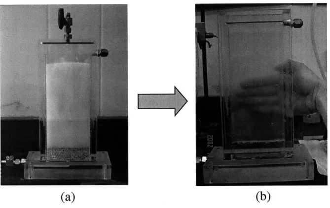
Figure 3-1 Illustration of the immersion method: (a) The medium filled with 1mm diameter borosilicate beads; (b) the beads are saturated with the optical laser liquid with

the sam e refractive index. ... 99

Figure 3-2. Illustration of the visualization technique. The emitted light from the fluorscent particles is visible as a bright area in the right picture...100 Figure 3-3 Particle size distribution curve of the discrete particles used for the experiments.

... 1 0 1

Figure 3-4 The single collector efficiency with different particle sizes at u=2.76x102 _cm/s

(m ed iu m )...10 2 Figure 3-5. Scanning electron microscope image of the particles. ... 103

Figure 3-6. Scanning electron microscope images of (a) the rough beads and (b) the sm o oth b ead s...104 Figure 3-7. Schematic diagram of the experimental box...105

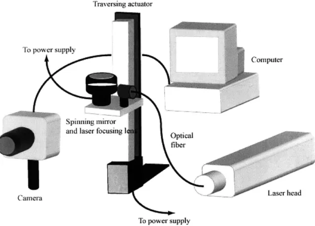
Figure 3-8. Particle injection system of the experimental setup...106 Figure 3-9. Particle excitation and capture system of the experimental set up...107 Figure 3-10. Laser light scanning using a polygonal spinning mirror. ... 108

Figure 3-11. Set up of the laser, the spinning mirror and the actuator for scanning the entire front face of the experimental box. Note that this figure is not to scale. ... 109 Figure 3-12. Picture of the whole experimental set up. ... 110

Figure 3-13. Captured images during experiment RM-1. Discrete particles were introduced into the medium at t=0. The presence of the discrete particles in indicated by "lighter" areas in the im ages. ... 111

Figure 3-14. Monitoring locations: (a) one in the source area; (b) through (h) seven inside the m edium ; (i) one in the breakthrough...112 Figure 3-15. A microscopic picture taken in the middle of the medium after the slow flow

rate test w ith the sm ooth beads, RS-2...113 Figure 4-1 Converting laser beam to a horizontal light sheet using (a) a Gaussian lens

attached to the laser outlet and (b) a spinning mirror...124 Figure 4-2 Non-uniformity of the light intensity in a horizontal light sheet when a Guassian

lens was used. (a), (b), and (c) show the movement of the high and low intensity locations at different times. Three images were captured at the same location, but at different tim es. ... 125

Figure 4-3 Light intensity fluctuation when the Gaussian lens was used...126 Figure 4-4 Uniformly distributed light using the spinning mirror. (a), (b), and (c) show

invariant light intensity at different tim es...127 Figure 4-5 Light uniformity at different locations when the spinning mirror was used.... 128 Figure 4-6 Light stability with time with or without laser unit warming-up process. ... 129 Figure 4-7 Concentration profile of the fluorescent particles deposited for the repeatability

te sts ... 1 3 0

Figure 4-8 Poor repeatability of data measurement when the Gaussian lens was used...131 Figure 4-9 Good repeatability of data measurements when the spinning mirror was used.

Figure 4-10 Light scattering effect: fluorescent light diffuses into its neighbor from a point so u rc e . ... 13 3

Figure 4-11 Experiment for the light scattering effect: (a) the medium was scanned without cover; (b) with a black cover at the top; (c) with a cover at the bottom; and (d) with covers both at the top and at the bottom. ... 134

Figure 4-12 Results of the light scattering effect experiment. When the black cover was used, the intensity of the area next to the cover is lower. ... 135

Figure 4-13 Monitoring areas to avoid the light scattering effect: (a) one in the source area;

(b) through (h) seven inside the medium; (i) one in the breakthrough. ... 136

Figure 4-14 Light penetration test. The light intensity was measured from a side of the experim ental box...137 Figure 4-15 Vertical light intensity calibration associated with the camera lens. ... 138 Figure 4-16 Two dimensional pixel by pixel calibration of each taken image caused by the

cam era len s...139

Figure 4-17 Calibration relationship to convert light intensity to colloid concentration... 140 Figure 4-18 Comparison of introduced particle mass with estimated particle mass for the

experim ent, R M -3. ... 14 1

Figure 4-19 Breakthrough results of the dye tests. D-1: u=4.26x10 2 _{cm/s; D-2:u=9.88x10-3}

cm/s. Dotted curve illustrates predicted breakthrough using an advection

dispersion equation with aL = 8.0 m m ... 142

Figure 5-1 Breakthrough curve of the particle transport tests at the three pore fluid velocities: (a) rough bead tests; (b) smooth bead tests. The solid lines are predictions from the Two-Site M odel...157 Figure 5-2 Breakthrough curve of the particle transport tests between pore volumes 0 and 5,

and comparison with solute breakthrough. The solute breakthrough is from dye tests and the estim ated dispersivity is 8m m . ... 158

Figure 5-3 Comparison of the plateau breakthrough concentrations for different flow velocities w ith both beads...159 Figure 5-4 Irreversible attachment rate of Two-Site Model estimated from the

breakthrough data...160 Figure 5-5 Reversible attachment and detachment rates of Two-Site Model estimated from

Figure 5-6 Particle size distribution of influent and effluent at different pore volumes for experim ent R S -3...162 Figure 5-7 Interior concentration change with time for experiment RS-2: (a) 1.8 cm from

the surface where particles are introduced; (b) 3.6 cm; (c) 5.8 cm; (d) 8.0 cm; (e) 12.4 cm; and (f) 15.0 cm. The solid lines represent predictions by Equations (4) and (6) using parameters obtained from the BTC. ... 163

Figure 5-8 Typical profile of measured interior concentration change with time. ... 164 Figure 5-9 Particle entrapment concentration for the fast flow velocity as a function of

surface roughness...165 Figure 5-10 Particle entrapment concentration for the medium flow velocity as a function

of surface roughness...166 Figure 5-11 Particle entrapment concentration for the slow flow velocity as a function of

surface roughness...167 Figure 5-12 Particle hindrance concentration for the fast flow velocity as a function of

surface roughness...168 Figure 5-13 Particle hindrance concentration for the medium flow velocity as a function of

surface roughness...169 Figure 5-14 Particle hindrance concentration for the slow flow velocity as a function of

surface roughness...170 Figure 5-15 Particle entrapment concentration for the smooth beads as a function of flow

v elo city ... 17 1

Figure 5-16 Particle entrapment concentration for the rough beads as a function of flow v elo city ... 17 2

Figure 5-17 Particle hindrance concentration for the smooth beads as a function of flow v elo city ... 17 3

Figure 5-18 Particle hindrance concentration for the rough beads as a function of flow v elo city ... 17 4

Figure 5-19 Microscopic observation of particle hindrance and entrapment while they were moving along with the pore water at V=1.27x10-2 cm/s (RS-micro). (a), (b), and (c) were taken during the particle introduction while (d), (e), and (f) during the flushing. (a) 0.9 pore volume passed; (b) 2.8 pore volumes passed; (c) 9.2 pore volumes passed (the end of the particle introduction); (d) 1.8 pore volumes

flushed after the end of the particle introduction; (e) 4.6 pore volumes flushed; and (f): 8.3 pore volumes flushed (the end of the flushing)...175 Figure 5-20 A microscopic picture taken in the middle of the medium after the slow flow rate test with the smooth beads, SS-3. Note that the black and white colors are reversed in the figure to make the entrapped particles visible more clearly.... 176 Figure 5-21 Breakthrough concentration of R3-2 when the pore water velocity was

increased to 2 and 4 times the initial velocity during the flushing. The eluted mass due to the hydrodynamic perturbation was less than 2% of the total

retained m ass... 177 Figure 6-1 Microscopic image of entrapped particles at the end of the microscopic test with

rough beads. CE refers to contact entrapment and SE refers to surface entrapment. Note that the black and white colors are reversed in the figure to make the entrapped particles visible more clearly. ... 194 Figure 6-2 Typical profile of measured interior concentration change with time.

Entrapment is calculated from the plateau concentration at Phase D, and

hindrance is calculated from the concentration decrease during Phase C. 195 Figure 6-3 Particle contact entrapment concentration as a function of velocity and depth

from the particle injection point...196 Figure 6-4 Hypothetical Distribution of Contact Entrapped Particles: (a) close to the

particle injection point; (b) lower in the medium ... 197 Figure 6-5 Particle contact entrapment concentration normalized by C - as a function

of depth from the particle injection point...198 Figure 6-6 Hypothetical view of surface entrapment: physical interlocking on surface

roughness. Fvdw is the van der Waals force between the discrete particle and the glass bead surface and 0 is the angular position of the surface roughness. ... 199 Figure 6-7 Microscopic images supporting the hypothesis of physical interlocking on

surface roughness for surface entrapment: (a) particles are entrapped on the surface of the glass beads with the rough beads; (b) particles are only entrapped at solid-solid contact points without surface entrapment for the smooth beads.

... 2 0 0

Figure 6-8 Schematic description of a porous medium based on the Happel's sphere in cell model [Happel, 1958]. The picture is taken from Ryan and Elimelech [1996].

Figure 6-9 Shcematic diagram of the overturning torque calculations for surface

en trapm ent...20 2 Figure 6-10 Torque balance calculation of surface entrapment for particles of a 10 ptm

diameter with a gap distance of 1 jim for the "slow" flow velocity tests. ... 203 Figure 6-11 0_crit

calculations as a function of particle diameter and flow velocity when (a)

h=0.5ptm , (b) h= Ipm , and (c) h=1.5gm . ... 204

Figure 6-12 Particle surface entrapment concentration as a function of flow velocity and depth from the particle injection point...205 Figure 6-13 hcrit calculations as a function of particle diameter and flow velocity when (a)

0=5', (b) 0=100, (c) 0=15', and (d) 0=20 . ... 206

Figure 6-14 Hindrance concentrations as a function of surface roughness and depth: (a) fast velocity; (b) medium velocity; (c) slow velocity. ... 207

Figure 6-15 Hindrance concentrations during the smooth bead tests: (a) the absolute

values; (b) the values normalized by C -NG 0.5 ... 208

Figure 6-16 Hindrance concentrations during the rough bead tests: (a) the absolute values;

(b) the values normalized by C -NG 0.5 ... 209

Figure 7-1 Comparison of entrapment and hindrance concentrations for the rough bead tests between the experimental measurements and the model fittings by Two-Site Model with the parameter values estimated from breakthrough: (a)

entrapment for fast tests, (b) hindrance for fast, (c) entrapment for medium, (d) hindrance for medium, (e) entrapment for slow, and (f) hindrance for slow tests.

... 2 3 4

Figure 7-2 Comparison of entrapment and hindrance concentrations for the smooth bead tests between the experimental measurements and the model fittings by Two-Site Model with the parameter values estimated from breakthrough: (a)

entrapment for fast tests, (b) hindrance for fast, (c) entrapment for medium, (d) hindrance for medium, (e) entrapment for slow, and (f) hindrance for slow tests.

... 2 3 5

Figure 7-3 Entrapment rate with depth across the medium for the rough bead tests: (a) Fast flow velocity, (b) m edium , and (c) slow...236 Figure 7-4 Entrapment rate with depth across the medium for the smooth bead tests: (a)

Figure 7-5 Contact entrapment rate and surface entrapment rate as a function of transport distance for each flow velocity: (a) Fast flow velocity, (b) Medium flow

velocity, and (c) Slow flow velocity. ... 238 Figure 7-6 Particle size distribution curves of the input solution and the output solution at

the end of the particle injection stage...239 Figure 7-7 Particle collection rate by entrapment for each particle size: (a) Entrapment

collection rate vs. particle diameter, and (b) Entrapment collection rate vs. settlin g velocity ... 240 Figure 7-8 Overall reentrainment rate of entrapment particles as a function of flow velocity and surface roughness...24 1 Figure 7-9 Example of the data fitting to obtain local collection and reentrainment rates

associated with particle hindrance. This is at 10.94 cm from particle injection point during a rough bead test at the medium flow velocity. The solid line is the model calculation using the parameter values estimated from the breakthrough data. The dashed line is the new local model fitting to obtain the hindrance and entrapm ent rates at the particular location. ... 242 Figure 7-10 Ratio between collection and reentrainment rates of particle hindrance

behavior inside the medium for the rough bead tests. The calculations were done with two different methods: 1. from the hindrance concentrations inside the medium and 2. from the calculated values by local model fittings as in T ab le 6 -3 . ... 24 3

Figure 7-11 Ratio between collection and reentrainment rates of particle hindrance behavior inside the medium for the smooth bead tests. The calculations were done with two different methods: 1. from the hindrance concentrations inside the medium and 2. from the calculated values by local model fittings as in T ab le 6 -3 . ... 24 4

Figure 7-12 Normalized particle breakthrough concentrations of different particle sizes at 2, 4, 6, 8, and 10 pore volum es. ... 245

Figure 7-13 Back-calculated breakthrough concentrations for the rough bead tests using the overall rates of entrapment and hindrance behavior averaged over the whole length of the medium. The values are compared with the experimental

breakthrough data and the fitting of the experimental data with Two-Site Model.

... 2 4 6

Figure 7-14 Back-calculated breakthrough concentrations for the smooth bead tests using the overall rates of entrapment and hindrance behavior averaged over the whole length of the medium. The values are compared with the experimental

breakthrough data and the fitting of the experimental data with Two-Site Model.

... 2 4 7

Figure 7-15 Modeling results from the Entrapment-Hindrance Model with rate distribution for the breakthrough concentration of slow test with the rough beads, and comparison with the Two-Site Model fitted directly with the breakthrough data.

... 2 4 8

Figure 7-16 Modeling results from the Entrapment-Hindrance Model with rate distribution for the peak concentration of Phase B and the plateau concentration of Phase D for the slow test with the rough beads and comparison with the Two-Site Model fitted w ith the breakthrough data. ... 249

Figure 7-17 Modeling results from the Entrapment-Hindrance Model with rate distribution for the hindrance concentration of the slow test with the rough beads and

comparison with the Two-Site Model fitted with the breakthrough data. ... 250 Figure 8-1 Comparison between the breakthrough of the upward tests and that of the

downward tests. The downward test data are from the rough bead tests with the medium velocity: (a) ALL TEST; (b) PV 0 TO 5...263 Figure 8-2 Breakthrough concentrations of the rough beads and the smooth beads for the upward tests. The solid line represents the model fitting...264 Figure 8-3 Microscopic image taken after the test, RU-1, in the middle of the medium. .265 Figure 8-4 Some examples of the interior concentration measurements with time for both

the rough beads and the smooth beads: (a) 1.75 cm distant from the source; (b)

5.85 cm; (c) 10.12 cm; and (d) 14.80 cm. The solid lines represent the model

predictions with the parameters estimated from the breakthrough data. ... 266 Figure 8-5 Typical profile of measured interior concentration with time for the upward

transport experim ents...267 Figure 8-6 Collection rate of particle entrapment as a function of distance, flow direction,

and surface roughness for the medium flow velocity. ... 268

Figure 8-7 Reentrainment rate of entrapped particles as a function of distance, flow

direction, and surface roughness for the medium flow velocity. ... 269 Figure 8-8 Concentration decrease during Phase C as a function of elevation and

comparison with the model calculations. Note, that the bottom of the box is the input area and the top of the box is the breakthrough area. ... 270

Figure 8-9 Peak concentration at the end of Phase B as a function of elevation and com parison with the m odel calculations...271

Figure 8-10 Ascending slope of Phase B as a function of elevation. The slope is a

representative of the collection rate of entrapment. The solid line is the model calculation. ... 272 Figure 8-11 Descending slope of Phase D as a function of elevation. The slope is a

representative of the reentrainment rate of entrapped particles. The solid line is the model calculation.273 Figure 9-8 Final particle distribution at the end of the drainage tests for each g-level... ... 294 Figure 9-1 Conceptual model of film straining (from Wan and Tokunaga [1997]). ... 288 Figure 9-2 Principle of centrifuge m odeling...289 Figure 9-3 Set up of the platform for the centrifuge experiments...290 Figure 9-4 Final particle distribution at the end of the drainage tests for each g-level...291 Figure 9-5 Retained mass fraction of the particles after the drainage tests for each g-level.

... . - ... ---.. .2 9 2

Figure 9-6 Residual saturation of the porous medium after the drainage tests for the g-levels ig an d 2 5 g ... 29 3 Figure 9-7 Sequential microscopic images while the pore water was being drained at ig: (a)

initially saturated with particle suspension; (b) when the air-water interface was passing; and (c) after the air-water interface passed. ... 294 Figure 9-8 Final particle distribution at the end of the drainage tests for each g-level...295

A-i Mass balance calculations

balance calculations balance calculations balance calculations balance calculations balance calculations balance calculations balance calculations balance calculations during RF-1...313 during RF-2...313 during RM -1. ... 314 during RM -2. ... 314 during RM -3. ... 315 during RM -4. ... 315 during RS-1...316 during RS-2...316 during RS-3...317 Figure Figure Figure Figure Figure Figure Figure Figure Figure A-2 A-3 A-4 A-5 A-6 A-7 A-8 A-9 Mass Mass Mass Mass Mass Mass Mass Mass

Figure Figure Figure Figure Figure Figure Figure Figure Figure Figure Figure Figure Figure Figure Figure Figure Figure Figure A-10 Mass A-Il Mass A-12 Mass A-13 Mass A-14 Mass A-15 Mass A-16 Mass A-17 Mass A-18 Mass A-19 Mass A-20 Mass A-21 Mass A-22 Mass A-23 Mass A-24 Mass A-25 Mass A-26 Mass A-27 Mass balance balance balance balance balance balance balance balance balance balance balance balance balance balance balance balance balance balance

Figure B-i Particle breakthrough concentrations with the rough beads at the fast flow velocity (RF): (a) raw data from each test and (b) averaged value. Note that the change from the particle injection stage to the particle flushing stage is adjusted to 10 P V s for (b )...327 Figure B-2 Particle breakthrough concentrations with the rough beads at the medium flow

velocity (RM): (a) raw data from each test and (b) averaged value. Note that the change from the particle injection stage to the particle flushing stage is adjusted to 10 P V s for (b )...32 8

calculations during R3-1...317 calculations during R3-2...318 calculations during SF-i...318 calculations during SF-2...319 calculations during SF-3...319 calculations during SM -1...320 calculations during SM -2...320 calculations during SM -3...321 calculations during SM -4...321 calculations during SM -5...322 calculations during SS-1...322 calculations during SS-2...323 calculations during SS-3...323 calculations during S3-1. ... 324

calculations during RU-1...324 calculations during RU-2...325 calculations during SU-1. ... 325

Figure B-3 Particle breakthrough concentrations with the rough beads at the slow flow velocity (RS): (a) raw data from each test and (b) averaged value. Note that the change from the particle injection stage to the particle flushing stage is adjusted to 10 P V s for (b )...329 Figure B-4 Particle breakthrough concentrations with the smooth beads at the fast flow

velocity (SF): (a) raw data from each test and (b) averaged value. Note that the change from the particle injection stage to the particle flushing stage is adjusted to 10 P V s for (b )...330 Figure B-5 Particle breakthrough concentrations with the smooth beads at the medium

flow velocity (SM): (a) raw data from each test and (b) averaged value. Note that the change from the particle injection stage to the particle flushing stage is adjusted to 10 PV s for (b). ... 331 Figure B-6 Particle breakthrough concentrations with the smooth beads at the slow flow

velocity (SS): (a) raw data from each test and (b) averaged value. Note that the change from the particle injection stage to the particle flushing stage is adjusted to 10 P V s for (b )...332 Figure B-7 Particle breakthrough concentrations of the three step flushing tests with the

rough b ead s (R 3)...333 Figure B-8 Particle breakthrough concentrations of the three step flushing test with the

sm ooth beads (S3-1)...333 Figure B-9 Particle breakthrough concentrations of the upward flow tests with the rough

beads (RU): (a) raw data from each test and (b) averaged value...334 Figure B-10 Particle breakthrough concentrations of the upward flow tests with the smooth

beads (SU): (a) raw data from each test and (b) averaged value. ... 335 Figure C-1 Temporal change of particle concentration inside the medium with the rough

beads at the fast flow velocity (RF): (a) 2.29cm, (b) 4.32cm, (c) 6.52cm, (d) 8.60cm, (e) 10.89cm, (f) 12.97cm, and (e) 15.42cm from the injection point.337 Figure C-2 Temporal change of particle concentration inside the medium with the rough

beads at the medium flow velocity (RM): (a) 1.94cm, (b) 4.28cm, (c) 6.52cm,

(d) 8.61cm, (e) 10.91cm, (f) 13.04cm, and (e) 15.49cm from the injection point. ... 3 3 9

Figure C-3 Temporal change of particle concentration inside the medium with the rough beads at the slow flow velocity (RS): (a) 1.84cm, (b) 3.83cm, (c) 5.99cm, (d) 8.22cm, (e) 10.43cm, (f) 12.50cm, and (e) 14.93cm from the injection point.341

Figure C-4 Temporal change of particle concentration inside the medium with the smooth beads at the fast flow velocity (SF): (a) 2.3 1cm, (b) 4.74cm, (c) 6.96cm, (d) 8.93cm, (e) 11.27cm, (f) 13.35cm, and (e) 15.62cm from the injection point.343 Figure C-5 Temporal change of particle concentration inside the medium with the smooth

beads at the medium flow velocity (SM): (a) 1.74cm, (b) 3.92cm, (c) 6.29cm,

(d) 8.49cm, (e) 10.76cm, (f) 12.81cm, and (e) 15.17cm from the injection point. ... 3 4 5

Figure C-6 Temporal change of particle concentration inside the medium with the smooth beads at the slow flow velocity (SS): (a) 1.93cm, (b) 4.04cm, (c) 6.42cm, (d)

8.61cm, (e) 10.81cm, (f) 12.96cm, and (e) 15.26cm from the injection point.347 Figure C-7 Temporal change of particle concentration inside the medium during the three

step flushing test with the rough beads, R3-1: (a) 1.64cm, (b) 3.46cm, (c) 5.59cm, (d) 7.88cm, (e) 10.14cm, (f) 12.24cm, and (e) 14.83cm from the

injection p oint. ... 34 9

Figure C-8 Temporal change of particle concentration inside the medium during the three step flushing test with the rough beads, R3-1: (a) 2.04cm, (b) 4.41cm, (c) 6.64cm, (d) 8.79cm, (e) 10.86cm, (f) 12.86cm, and (e) 14.95cm from the

injection p o in t. ... 3 5 1

Figure C-9 Temporal change of particle concentration inside the medium for the upward flow tests with the rough beads (RU): (a) 1.70cm, (b) 3.80cm, (c) 5.83cm, (d) 7.87cm, (e) 10. 10cm, (f) 12.32cm, and (e) 14.80cm from the injection point.353 Figure C-10 Temporal change of particle concentration inside the medium for the upward

flow tests with the smooth beads (SU): (a) 1.80cm, (b) 3.81cm, (c) 5.87cm, (d) 7.92cm, (e) 10.14cm, (f) 12.40cm, and (e) 14.79cm from the injection point.355

List of Tables

Page

Table 3-2 Fluorescence properties of the organic dyes embedded in the particles [Guilbault,

19 9 0 ]. ... 9 7

Table 3-3. Details of the experiments conducted... 98

Table 4-1 Mass balance calculations during each experiment...123 Table 5-1 Parameter values of Two-Site Model estimated by fitting the particle

breakthrough data to the m odel...155 Table 5-2 Fractions of the particles entrapped and hindered during the experiments...156 Table 7-1 The averaged entrapment rates over the medium for each test and comparison

with the irreversible rates from Two-Site Model...227 Table 7-2 The overall surface entrapment and contact entrapment rates for the rough beads

for each flow velocity...228 Table 7-3 Reentrainment rates of entrapped particles at each location inside the medium

for the different test conditions. The overall value is the one averaged over the entire length of the m edium . ... 229

Table 7-4 Collection and reentrainment rates of hindrance behavior at each location for different test conditions. The overall values are the averaged values over the whole length of the medium. The values estimated from the breakthrough data using Tw o-Site M odel are also listed...230 Table 7-5 Overall ratio between collection and reentrainment rates of particle hindrance for

each test con dition ... 23 1

Table 7-6 Rough estimation of in kre for different particle sizes by looking at the

hin

breakthrough curves...232

k k"'

Table 7-7 r k or hin k-01 calculations for each test condition. ... 233

irr ent

CHAPTER 1

INTRODUCTION

1.1. MOTIVATION

Discrete particles are particles whose sizes are in the range of submicron to micron. Different kinds of discrete particles, present in the environment - air, water, and soil, affect

living organisms including human beings. For example, particulate matters or aerosols small enough not to be seen by human eyes are serious air pollutants. In addition,

chemicals and microorganisms, present in water and soil in the form of colloidal particles cause contamination and can adversely impact human health. The focus of this research is the behavior of discrete particles in porous media.

An understanding of discrete particle behavior in porous media is important to a number of problems involving subsurface flow and transport, water and wastewater treatment, soil pedology, and medical treatment. For example, colloid particles, a group of discrete particles operationally defined as having effective diameters ranging from 1 nm to 10 ltm

[Chrysikopoulos and Sim, 1996], are thought to facilitate the subsurface migration of both organic and inorganic contaminants [McCarthy and Zachara, 1989; Penrose et al., 1990; Ryan and Elimelech, 1996]. Recently, "functionally intelligent" particles with sizes in the sub-micron to micron range are now being considered as possible aids to subsurface characterization and remediation [Mackay and Gschwend, 2001]. Furthermore, the

subsurface transport of viruses, bacteria and protozoa such as Cryptosporidium parvum, a spherical shape oocyst with an average diameter of 5 ptm, also appear to exhibit features of discrete particle transport [Harter et al., 2000]. In water and wastewater treatment, filtration through granular media is extensively used to remove micron-sized particles from liquid input streams [Aim et al., 1997], while work in the field of soil pedology attributes the

formation of argillic horizons to the translocation of dilute clay suspensions [Hopkins and Franzen, 2003]. In addition, filtration technologies are also used in the filtration of blood

to remove infected blood cells in a clinical or diagnostic way [Burnouf and Radosevich, 2000; Jones et al., 1994; Kapadia et al., 1992; Steneker et al., 1995]. Some of these problems are described in more detail in the following paragraphs.

The idea that colloid particles in groundwater enhance contaminant transport has

attracted wide spread attention recently. A review paper published in 1989 pointed out that mobile colloids in groundwater could be possible agents for carrying contaminants, owing to the strong tendency for contaminants to adsorb onto colloid particles [McCarthy and Zachara, 1989]. In addition, organic and inorganic contaminants believed to be associated with colloid particles have been observed at some field sites to move in the subsurface faster than predicted [Ryan and Elimelech, 1996; Roy and Dzombak, 1997, 1998]. This idea has since been investigated and proven experimentally in laboratory work [e.g., Ryan

and Elimelech, 1996] and field work [McCarthy et al., 1998a; McCarthy et al., 1998b; Penrose et al., 1990]. It has also been demonstrated numerically with computer simulations

[Corapcioglu and Jiang, 1993a, 1993b; Prechtel et al., 2002], and is now considered a "fact" rather than a "hypothesis" [Honeyman, 1999; Kersting et al., 1999].

In addition to facilitating contaminant transport, colloids might also be useful agents for groundwater remediation. Because of their ability to remain stable in groundwater flow under certain chemical and physical conditions, colloid particles could offer a potential means of delivering remedial agents (e.g. surfactants) to contaminated sites more effectively than injection of the remedial agent alone [Brenner and Edwards, 1993]. For example, a recent study demonstrated the feasibility of using colloid particles, which were manipulated by perturbing the geochemical conditions, as a contaminant sorbent [Johnson et al., 2001].

The migration of various microorganisms along with groundwater in the subsurface as well as pathogens can be a significant environmental problem [Ginn et al., 2002; Harter et al., 2000]. In addition, microorganisms can be used as a remedial tool for contaminated soil and groundwater, known as so-called bio-remediation [National Research Council,

microorganism transport as discrete particles in porous media is critical to the prevention of groundwater contamination and the design and implementation of bioremediation schemes [Ginn et al., 2002].

Filtration through porous media is widely used for water and wastewater treatment [American Water Works Association, 1999] and for medical treatment [Kapadia et al.,

1992]. Discrete particles flowing through a porous medium along with interstitial fluid are

filtered inside the medium by physical and chemical mechanisms. Knowledge of the mechanisms governing discrete particle behavior during filtration is required to enhance the implementation and control of these filtration techniques.

1.2.

PROBLEM STATEMENT

Because of the importance of discrete particle behavior in porous media in numerous environmental applications, a great deal of experimental and mathematical research has been done on this subject. Consequently, there has been much progress towards

understanding discrete particle behavior in porous media, especially over the last decade or so. Nonetheless, many challenges still remain, some of which are highlighted below.

The so-called "filtration theory" has been most widely used to predict the behavior of suspended and colloidal particles in porous media [Elimelech et al., 1995; Tien, 1989]. This theory uses a simplified mathematical approach to obtain a macroscopic filtration efficiency for particle attachment on the soild phase of the porous medium. Happel's sphere-in-cell model is used to represent the porous medium as a system of identical spherical "collectors" surrounded by individual fluid envelopes [Happel, 1958]. A single collector efficiency is then calculated for each cell and converted to a macroscopic parameter that is termed the filtration coefficient. Although this method has been

successfully used in numerous studies [Elimelech et al., 1995; Ryan and Elimelech, 1996; Ryan et al., 1999; Tien, 1989], the theory assumes an idealized porous medium, so it is limited with respect to its application to real situations.

Many studies that experimentally investigate discrete particle behavior in a porous medium involve using a laboratory column packed with a porous medium. Particles are

then introduced into the column inlet and particle concentrations are monitored at the column outlet [e.g., Bradford et al., 2002; Compere et al., 2001; Gamerdinger and Kaplan, 2001; Kretzschmar and Sticher, 1998; Litton and Olson, 1993; Saiers et al., 1994a; Saiers et al., 1994b]. The monitored breakthrough concentration is then fitted with a mathematical model, in which the particle attachment mechanisms are described using the filtration theory. Thus, these studies concede to the assumptions of the filtration theory without making any direct observations of particle behavior. To overcome this limitation of column experiments, a destructive way of looking inside the medium was used in some studies. In order to do this, a porous medium column was disassembled and the particle concentration

distribution was measured inside the medium after a particle transport experiment through the column was finished. This destructive sampling has, in fact, shown that model

predictions calculated from fitting the breakthrough curve didn't agree with the interior concentration distribution inside the medium, because the particle attachment was

observed to be higher than predicted in the medium close to the particle inlet [Bolster et al.,

1999; Bradford et al., 2002; Redman et al., 2001]. However, even in these studies, the

particle behavior inside the medium was not observed directly, instead the sampling revealed the concentration distribution only once - at the end of the tests. In addition, the

destructive sampling method caused specimen and data disturbance, and led to poor particle mass recovery. A real-time and non-destructive, direct observation method is required to advance current methods for studying particle behavior in porous media.

Attempts have been made to directly observe particle movement in porous media, either using so-called "micro-models", which utilize photochemically etched glass plates to simulate porous media [Lanning and Ford, 2002; Sirivithayapakorn and Keller, 2003; Wan et al., 1996; Wan and Wilson, 1994], or the immersion method [Ghidaglia et al., 1996a,

1996b], which creates an optically transparent medium. Micromodels have limitations

because they cannot represent the three dimensional features of pore space that are

believed to affect particle behavior. The immersion method involves the use of an organic pore fluid, so particle behavior in immersion experiments might not be representative of particle behavior in aqueous solution.

Work in the Physics literature [Ghidaglia et al., 1996a, 1996b; Lee and Koplik, 1999] has clearly illuminated the impact microscopic particle behavior has on macroscopically observed trends in discrete particle transport. Evidence for particle capture at both

geometric and hydrodynamic sites has been provided, in addition to evidence of the "re-launching" of captured particles by other by-passing particles, the "hesitation" of particles at bifurcating stream-lines, and the "waiting" of particles in pore bodies before they exit via a pore throat. This work has also shown that these phenomena are influenced by the direction of the pore fluid velocity. Directional flow dependence and the other

aforementioned phenomena are not accounted for in the work cited in the above paragraphs.

Even in mathematical simulation approaches, several different mechanisms are used to explain discrete particle behavior. The most popular approach is one that assumes

first-order attachment rate for particle filtration by the medium. Other approaches incorporate particle detachment, dynamic blocking effects, multi-rate attachment and detachment sites,

and so forth [Compere et al., 2001; Gamerdinger and Kaplan, 2001; Johnson and

Elimelech, 1995; Kretzschmar and Sticher, 1998; Saiers et al., 1994a; Saiers et al., 1994b; Schaaf and Talbot, 1989; Yan, 1996]. No experimental, field and/or theoretical study has provided a robust guideline for the different mechanisms of particle behavior applicable to each situation. Instead, these mechanisms are usually assumed and applied in models without direct observations.

This research was initiated based on the limitations identified above with the current predictive and experimental methods. The research was planned and motivated by the following arguments:

1. The complex three-dimensional features of pore space and hydrodynamic flow fields, such as grain-grain contact points and fluid stagnation points, affect particle behavior in a porous medium. These features are not accounted for in current predictive and experimental methods.

2. Particle behavior inside porous media is not uniform, but contains variance that can be brought about by physical variables such as hydrodynamic forces, gravity forces, particle sizes and shapes.

3. The behavior of discrete particles inside a porous medium is influenced by local physical and chemical factors while they are moving, so in order to understand particle behavior, the particle movement must be directly observed and the

dependence on the influential factors must be quantified to improve understanding in this area.

1.3. OBJECTIVES AND SCOPE OF RESEARCH

This thesis presents work that has been conducted to further understanding of the

mechanisms governing the behavior of discrete particles in the interior of a uniform porous medium. The motivation for the work is to provide insight that can be used to improve existing, commonly used approaches to modeling discrete particle fate and transport in porous media. The detailed objectives of this work were to:

1. Directly visualize discrete particles moving in the interior of a porous medium during particle transport.

2. Use the visualization technique to elucidate the macroscopic and microscopic behavior of negatively charged non-Brownian particles in a uniform, saturated medium.

3. Understand the influence of physical factors, including three dimensional pore features, flow velocity, gravity, particle size, and solid surface roughness, on the behavior of the particles in the medium.

4. Provide guidelines for improving mathematical models for predicting discrete particle behavior in porous media.

To meet these objectives, a new experimental technique was developed for visualizing particle transport in the interior of a porous medium. This technique was used to examine the behavior of negatively charged, non-Brownian particles in the interior of a medium constructed from mono-size 4mm diameter glass beads saturated with distilled/deionized water. Both macroscopic and microscopic particle behavior were observed as a function of

pore fluid velocity, bead surface roughness, and flow direction. The results of the work reveal particle behavior not accounted for by the filtration theory and any other studies published so far.

1.4. THESIS ORGANIZATION

This thesis is divided into ten separate chapters. The contents of each chapter are summarized as follows.

Chapter 1, the current chapter, introduces the motivation for the research, highlights some problems associated with current predictive and experimental methods, and states the objectives of the research.

Chapter 2 provides background material on discrete particle behavior in porous media. Current existing theories and various experimental approaches are described. Discrete particle transport mechanisms, DLVO theory and the filtration theory are explained in detail.

Chapter 3 and Chapter 4 present the newly developed experimental method, namely the new visualization technique. Chapter 3 describes the new technique and the equipment used. In addition, the detailed experimental set up and procedure are discussed. The materials that were used for the experiments are also described in this chapter. Chapter 4 discusses how well the experimental method performs. The calibration method, data stability and repeatability are all discussed. Mass balance calculations, as another means of checking the reliability of the method, are also presented. Dye tests to approximate the dispersivity of the medium are also provided.

Chapter 5 and Chapter 6 discuss the behavior of downward discrete particle transport in the porous medium. Chapter 5 provides the macroscopic observations, illustrating the main characteristics and mechanisms suggested by the observations, and the microscopic images of the mechanisms and how they work at a microscopic scale. Comparisons between the macroscopic and microscopic observations lead to important conclusions on discrete particle behavior in a porous medium that have not been reported in other studies. Chapter