Diamagnetic measurements on the Alcator C tokamak

PFC/RR-85-13 _{DOE/ET-51013-156} UC-20 a, b, d, f DIAMAGNETIC MEASUREMENTS ON THE ALCATOR C TOKAMAK

Thomas Donovan Shepard Plasma Fusion Center

Massachusetts Institute of Technology Cambridge, MA 02139

July 1985

This work was supported by the U.S. Department of Energy Contract No. DE-AC02-78ET51013. Reproduction, translation, publication, use and disposal, in whole or in part by or for the United States govern-ment is permitted.

DIAMAGNETIC MEASUREMENTS ON THE

ALCATOR C TOKAMAK by

Thomas Donovan Shepard B.S., Columbia University, 1982

Submitted to the Department of Electrical Engineering and Computer Science

in Partial Fulfillment of the Requirements of the Degrees of

MASTER OF SCIENCE and

ELECTRICAL ENGINEER at the

MASSACHUSETTS INSTITUTE OF TECHNOLOGY June 1985

@

Signature of Author

Department of Electrical Engineering and Computer Science June 3, 1985

Certified by

Professor Ronald R. Parker Thesis Supervisor

Accepted by

Professor Arthur C. Smith Chairman, Graduate Committee

DIAMAGNETIC MEASUREMENTS ON THE

ALCATOR C TOKAMAK by

Thomas Donovan Shepard B.S., Columbia University, 1982 Submitted to the Department of Electrical Engineering and Computer Science

in Partial Fulfillment of the Requirements of the Degrees of

MASTER OF SCIENCE and

ELECTRICAL ENGINEER at the

MASSACHUSETTS INSTITUTE OF TECHNOLOGY ABSTRACT

A procedure for determining the total thermal energy content of a magnetically confined plasma from a measurement of the plasma magnetization has been suc-cessfully implemented on the Alcator C tokamak. When a plasma is confined by a magnetic field, the kinetic pressure of the plasma is supported by an interaction between the confining magnetic field and drift currents which flow in the plasma. These drift currents induce an additional magnetic field which can be measured by means of appropriately positioned pickup coils. From a measurement of this magnetic field and of the confining magnetic field, one can calculate the spatially averaged plasma pressure, which is related to the thermal energy content of the plasma by the equation of state of the plasma.

The theory on which this measurement is based is described in detail. The fields and currents which flow in the plasma are related to the confining magnetic field and the plasma pressure by requiring that the plasma be in equilibrium, i.e., by balancing the forces due to pressure gradients against those due to magnetic interactions.

The apparatus used to make this measurement is described and some example data analyses are carried out. It turns out that the signal due to the induced plasma magnetization is very small compared to interference signals caused by other mag-netic systems in the tokamak. The work involved in the diamagmag-netic measurements was thus dominated by the necessity of accurately eliminating all the interference sources. These error signals were attributed to linkage of OH and EF fields, link-age of plasma toroidal current, magnetic diffusion effects, eddy currents induced in the vacuum chamber wall, fringing fields in the vicinity of the diamagnetic loops, compression of the magnet structure, and integrator drift. The methods used to eliminate these errors and some possible alternative methods are described.

Thesis Supervisor: Dr. Ronald R. Parker

UNITS

The system of units used in this paper is basically the MKS system. However, for convenience the Maxwell equations are written with the permeability of free space Ao set equal to unity. This is convenient because in the analyses of Chapters 1-4, IO is nothing more than a scale factor expressing the fact that different phys-ical dimensions are used to measure the magnetic field quantities B and H. So by setting po equal to one, the necessity of including it in complicated mathematical expressions is avoided. Of course, the quantity Ao is restored whenever present-ing equations that are actually used in makpresent-ing experimental measurements, since standard laboratory measurements are made in terms of real MKS units.

It is actually very easy to formally develop a system of units in which the per-meability of free space is equal to one. One way to do this is as follows: Express any velocity by the dimensionless number representing the velocity as a fraction of the speed of light in free space. Then define all electric field quantities by the force per unit charge exerted by the respective field on a test charge and define all mag-netic field quantities by the force per unit charge per unit (dimensionless) velocity exerted by the respective field on a moving test charge. Thus all electromagnetic field quantities have the dimensions of force per unit charge. The magnitude of the unit of charge then determines the proportionality constant appearing in the Gauss equation. If the unit of charge is selected in such a manner that the elec-tromagnetic equations are "rationalized", then the Maxwell equations take on the following simple form:

B V xE -= (U.1)

at

_at

The analysis of Chapters 2-4 makes extensive use of perturbation theory. The use of perturbation theory requires the identification of the "order" of every alge-braic term with i-espect to some "smallness"'parameter (E). This is greatly facili-tated by redefining all physical quantities so that they are represented by dimen-sionless numbers and choosing the scales of these numbers so that they are all zero order in e. This way the order of any term may immediately be determined simply by noting the algebraic power of E appearing in it.

TABLE OF CONTENTS ABSTRACT . . . ... .. . . . .. . . . . . UNITS . . . . TABLE OF CONTENTS ... CHAPTER 1: Introduction ... 1.1 Introduction . . . . 1.2 Simple Models of Plasma Diamagnetism . . . . 1.3 Description of a Tokamak . . . . 1.4 MHD Model of Plasma Equilibrium . . . .

CHAPTER 2: The Grad-Shafranov Equation for Plasma Equilibrium 2.1 Derivation of the Grad-Shafranov Equation . . . . .

2.2 Asymptotic Expansion of the Grad-Shafranov Equation 2.3 Zero. Order Solution of the Grad-Shafranov Equation 2.4 First Order Solution of the Grad-Shafranov Equation 2.5 Higher Order Corrections to the Poloidal Beta . . . .

. . . . . . . 20

. . . . . . . 24

. . . 28

. . . 30

. . . 32

CHAPTER 3: Tensor Representation of Plasma Equilibrium . . . 34

3.1 Derivation of the Total Pressure Tensor . . . 34

3.2 Solution for the Radial Pressure Balance . . . 36

3.3 Solution for the Toroidal Force Balance . . . 39

CHAPTER 4: Experimental Apparatus . . . 44

4.1 Overall Description of the System . . . . .. . . . 44

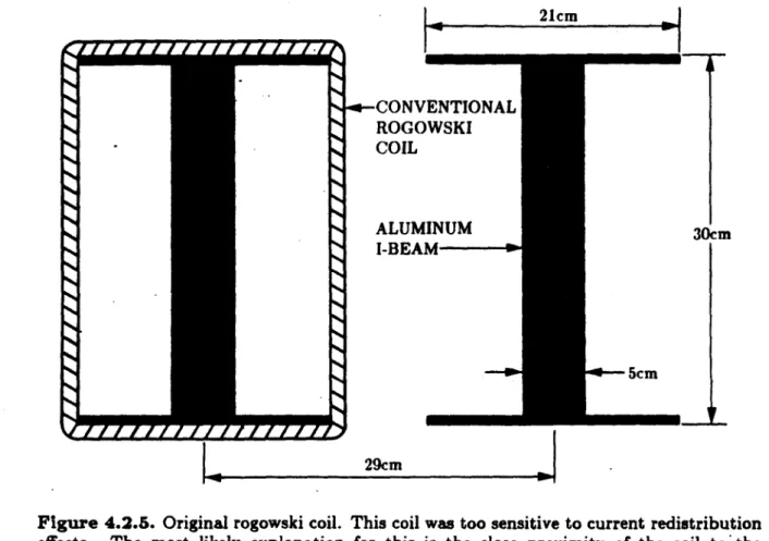
4.2 Precision Rogowski Coil . . . 46

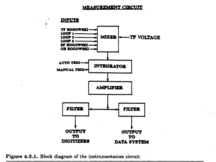
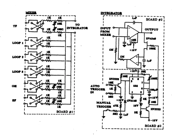
4.3 The Instrumentation Circuit . . . 53

CHAPTER 5: Some Experimental Results . . . 59

5.1 Calculation of the Energy Confinement Time . . . 59

5.2 Lower Hybrid Heating Results . . . 60

5.3 Pellet Injection Results . . . 64

CHAPTER 6: Systematic Errors . . . 69

6.1 Introduction . . . 69

6.2 Poloidal Eddy Currents . . . 74

6.3 Compression of the Magnet Structure . . . 88

CHAPTER 7: Summary . . . . . . . 9 1 . . . . 12

. . . . 18

. . . . 20

APPENDIX . . . .. . . . . . . . .. . . . . . 93

A.1 Characteristics of the Alcator C Tokamak . . . 93

A.2 Toroidal Coordinates . .. . .. _{. . . 95}

A.3

CHAPTER 1: Introduction

1.1 Introduction

A magnetically confined plasma by definition consists of a region of space oc-cupied by plasma under pressure, surrounded by a vacuum region containing a magnetic field. Since the plasma must not be allowed to come in contact with any other material, the forces which pressurize the plasma must come from an in-teraction between the confining magnetic field and induced currents which flow in the plasma. These induced currents will generate their own magnetic field - the plasma magnetization - which will oppose the confining field. Because the in-duced plasma magnetism always opposes the confining fields, the inin-duced currents are called the "diamagnetic drift current" and the resulting magnetic field is called "plasma diamagnetism".

Since plasma diamagnetism is a direct consequence of magnetic confinement, one might expect that a measurement of plasma diamagnetism would reveal information about the kinetic pressure of the plasma. This information might then be related to the thermal energy content of the plasma through the equation of state of the plasma.

Consider a cylindrically symmetric plasma column confined by an axial magnetic field, as illustrated in Fig. 1.1.1. In order to have a static equilibrium, the plasma pressure, current, and the total magnetic field (i.e., confining field plus plasma diamagnetism) must be related by

Vp = J x B, (1.1.1)

where p is the plasma kinetic pressure, J is the plasma current density, and B is the total magnetic field. Eq. (1.1.1) expresses a balance between the force due to pressure gradients and the Lorentz force at any point in the plasma. Since the plasma is assumed to be confined, Vp must point radially inward. Thus, according to Eq. (1.1.1), the diamagnetic drift current must be tangential, directed as shown in Fig. 1.1.1. By the right-hand rule, one can see that the resulting plasma magnetism is diamagnetic.

This paper describes the theoretical and experimental aspects of a plasma di-agnostic which uses the plasma magnetization as a measure of the thermal energy content of the plasma, and which has been successfully implemented on the Alcator C tokamak. The experimental apparatus for measuring plasma magnetization is

H

J

BD PLASMA

Vp

Figure 1.1.1. A cylindrically symmetric plasma column, confined by an axial magnetic field. H is the applied magnetic field, J is the diamagnetic drift current, B is the total magnetic field, and p is the plasma pressure. Given that Vp points inward, Eq. (1.1.1) requires that J be directed as shown. Note that the magnetization produced by J opposes the applied field H.

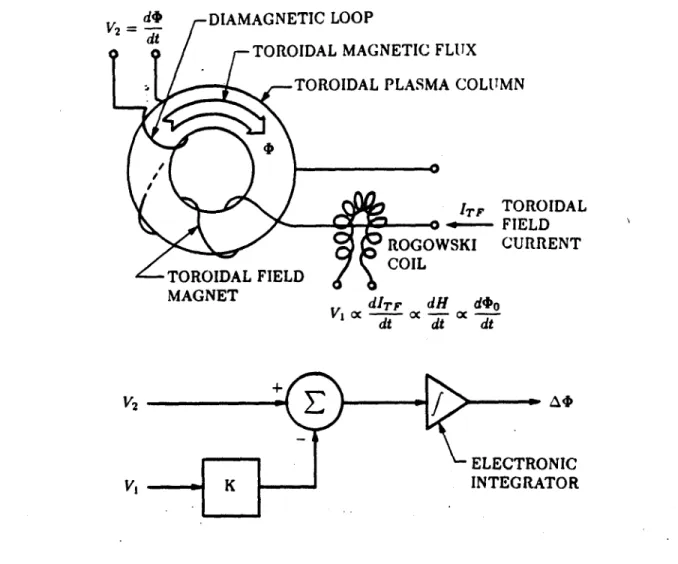
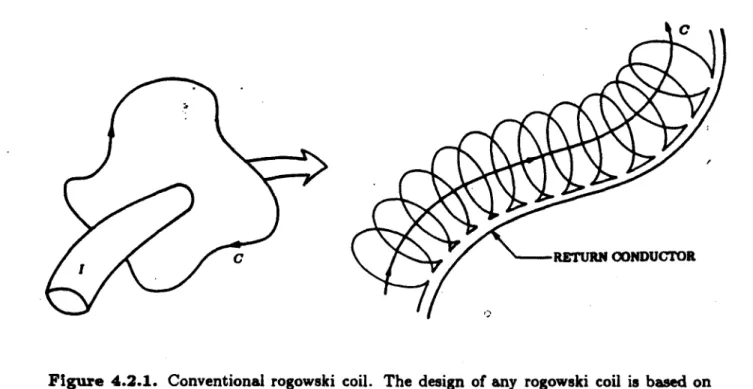
shown schematically in Fig. 1.1.2. The diamagnetic loop is a single-turn flux loop which links the total toroidal magnetic flux. The rogoweki coil links a magnetic flux which is proportional to the toroidal magnetic flux due to the vacuum (i.e.,

"ap-plied") magnetic field. The difference between these fluxes represents the magnetic

flux produced by the plasma. Since the terminal voltage of a flux loop is equal to the time derivative of the enclosed flux, these signals are integrated electronically to obtain a voltage signal proportional to the plasma magnetization.

In Fig. 1.1.2, the voltage produced by the diamagnetic loop is

V2 = (1.1.2)

dt

where t is the total toroidal magnetic flux. The voltage produced by the rogowski coil is

Vi oc -- (1.1.3)

dt

where to is the vacuum toroidal magnetic flux. Thus, by proper adjustment of the constant gain K, the output of the integrator will be

A = f (V2 - KV) dtizatio

V2 =d DIAMAGNETIC LOOP

di

TOROIDAL MAGNETIC FLUX TOROIDAL PLASMA COLUMN

ITF TOROIDAL ---- FIELD

ROGOWSKI CURRENT TOROIDAL FIELD

MAGNET _{dITF dH d$o}

di0 t- dC t

dt--V2

f

ELECTRONIC

V, K INTEGRATOR

Figure 1.1.2. Experimental apparatus for measuring plasma magnetization. 0 represents

the total toroidal magnetic flux during a plasma discharge, -to is the flux due to the vacuum field only, and A(P is the toroidal flux due to plasma magnetization.

1.2 Simple Models of Plasma Diamagnetism

This plasma diamagnetism can be shown to be directly related to the plasma pressure and, through the equation of state, to the plasma thermal energy. To illustrate this, I will describe two somewhat oversimplified models of the plasma that exhibit this behavior. In the first model, the plasma consists of a single charged particle in the presence of a magnetic field. In the second model, the plasma consists of a collection of noninteracting charged particles in the presence of a magnetic field. These models are too simple to be used to justify a theory that relates diamagnetism to pressure, because they ignore important plasma phenomena such as collective interactions between particles. However, they do serve to illustrate the phenomenon physically, without the burden of mathematical rigor. A more accurate model, which is based of an ideal magnetohydrodynamic description of

r

H q 4m

Figure 1.2.1. A single charged particle of mass m, charge q, gyrating in the presence of an applied vacuum field H. r is the radius of the orbit and vj. is the component of the velocity of the particle which is perpendicular to the magnetic field.

Consider a particle of charge q, mass m, and perpendicular kinetic energy

2112=g o (1.2.1)

in the presence of a constant, spatially uniform, applied magnetic field H (Fig. 1.2.1). The particle will undergo cyclotron motion, behaving like a magnetic dipole of moment

IA, (1.2.2)

where

I =q/T (1.2.3)

is the electric current due to the orbiting particle, and the orbital period is given by

T = 22r/n, (1.2.4)

where

f

is the erbital (cyclotron) frequency. The area of the orbit is

A = rr 2, (1.2.6)

and the orbital radius is

where v1 is the velocity component perpendicular to the applied magnetic field H.

These equations can be combined as follows

q v -= - = qv2 m _ 'mv± (1.2.8)

22 f 2 _{f2l 2 qH . H H}

showing that the magnetic moment of the particle is directly related to its perpen-dicular kinetic energy.

Now consider a spatially uniform plasma composed of several particle species, each with a distribution function that can be characterized by a temperature. If the particles do not interact magnetically with each other, the plasma magnetization will be given by

M = n

N

3

E

Z

J

mV2fj(v)d3v

H H H'

where j is the species index, nj is the particle density of species j, pij is the magnetic moment of a particle of species j and velocity v,

f,

PA

M

where h is a unit vector in the direction of the applied magnetic field, H. The total magnetic field in the plasma is

B=H+M = H 1 - = H(1+ Xm), (1.2.11)

where Xm = -P/H2 _{is the magnetic susceptibility.}

As was pointed out above, while these simple models may be physically re-vealing, they do not take into account interactions between particles. What they do show is that "plasma" diamagnetism is a property that is exhibited by both a

PLASMA SURFACE - - r=a, 0<9<27r, R 2 R TOROIDAL -MIDPLANE z=O

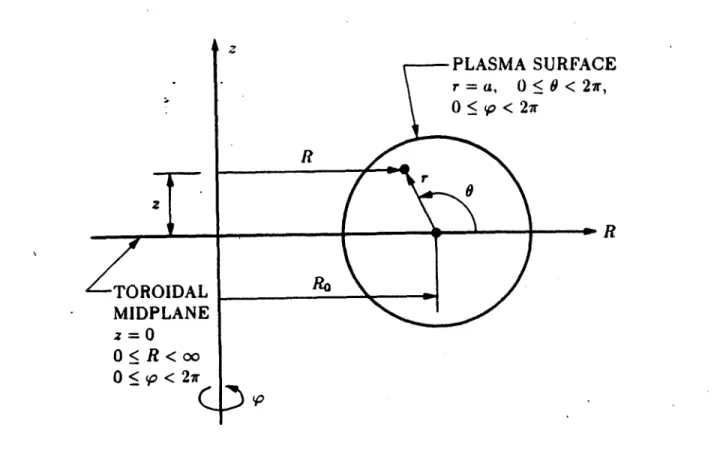
Figure 1.3.1. Toroidal geometry. This figure represents a poloidal section through the toroidal plasma column. The z-axis is the'vertical centerline of the tokamak and the plane z = 0 is the toroidal midplane of the tokamak. (R, (p, z) is a conventional cylindrical coordinate system while (r, V, 9).is the toroidal coordinate system to be used in this paper. RO is the major radius of the plasma and a is the minor radius of the plasma.

single, isolated particle, and a collection of noninteracting particles. A more sophis-ticated theory, based on a magnetohydrodynamic model of the plasma, is described in Chapters 2 and 3.

1.3 Description of a Tokamak

In a tokamak, the cylindrical plasma column is bent into the shape of a torus. The relevant geometry is illustrated in Fig. 1.3.1. The tokamak is symmetric about the z-axis. The distance from the z-axis to the center of the plasma is called the major radius of the plasma and is denoted by RO. The distance from the center of the plasma column to the surface of the plasma column is called the minor radius and is denoted by a.

The analysis in Chapters 2 and 3 will be carried out with reference to the two coordinate systems shown in Fig. 1.3.1. The cylindrical coordinate system (R, p, z) consists of the major radial coordinate, R, the vertical coordinate, z (distance above the toroidal midplane), and the toroidal angle, V. The toroidal coordinate sys-tem (r, p, 9) consists of the minor radial coordinate, r (distance from the center of

the plasma column), the poloidal angle, 6, and the toroidal angle, P. The plane p = constant is a two-.dimensional space called the poloidal plane. The poloidal

coordinates are (R, z)* in cylindrical coordinates, or (r, 6) in toroidal coordinates. The projection of any vector quantity, A, onto the poloidal plane is another vector called the poloidal component of A and is denoted by

Ap = A - A _(1.3.1)

where 0 is a unit vector in the toroidal direction and

A, = 0 -A. (1.3.2)

A, is called the toroidal component of A.

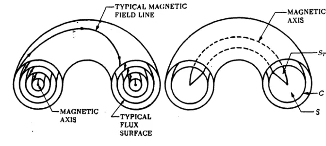
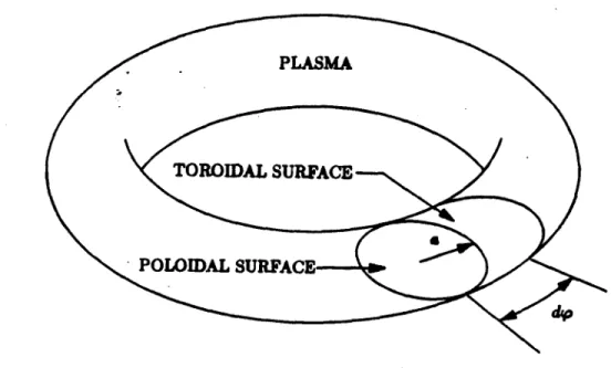
In a tokamak that can be described by ideal magnetohydrodynamic (MHD) theory, the magnetic field lines lie on nested toroidal surfaces as illustrated in Fig. 1.3.2. Thus, a characteristic of one of these surfaces is that no magnetic field lines cross it, and therefore that it encloses a certain well-defined magnetic flux. In particular, there will be a special innermost flux surface which encloses no flux at all. This surface will really be a single curve, called the magnetic axis of the tokamak. The intersection of a particular flux surface with the poloidal plane will be a curve C which spans a surface S. The magnetic flux through S is obviously the flux enclosed by the flux surface and is called the toroidal magnetic fluz associated with the flux surface. If one chooses the point in S which lies on the magnetic axis and any particular point on C and rotates these two points toroidally by one complete circuit, another surface ST is generated. Since no field lines cross the flux surface, the magnetic flux through ST is independent of the point chosen on C and is called the poloidal magnetic fluz associated with the flux surface.t Note that in ideal MHD, the electric current density is divergenceless, so that these same

definitions can be made in terms of the current flux and current flux surfaces. An important geometrical parameter that measures the degree of toroidicity of the plasma column is the aspect ratio, Ro/a. Since it is physically impossible to construct a torus with an aspect ratio less than unity, the inverse aspect ratio,

defined by

E = a/Ro (1.3.3)

* Note that (R, z) is a rectangular (Cartesian) coordinate system.

t In the analysis of Chapter 2 the quantity called the poloidal flux is actually this quantity divided by 27r, i.e., the poloidal flux per toroidal radian.

TYPICAL MAC FIELD LINE

MNETIC -TYPICAL FLUX SURFACE

Figure 1.3.2. Nested toroidal flux surfaces. The intersection of any particular flux surface with the poloidal plane defines a curve C which spans a surface S. The flux through S is called the toroidal flux associated with the flux surface. The poloidal flux associated with the flux surface is the flux through the surface ST which is generated when the line joining any particular point on C with the magnetic axis is rotated toroidally.

is a quantity that is always less than unity. This property is often exploited in

theoretical analyses by developing asymptotic expansions in series of powers of e.

In practical devices, the inverse aspect ratio is usually sufficiently small that only a few terms in a series are necessary to obtain a useful result.

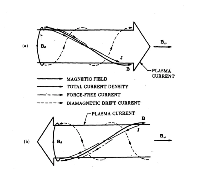
In a tokamak, in addition to the confining magnetic field and the diamagnetic drift current, there are other fields present, some of which are indicated in Fig. 1.3.3. The confining magnetic field consists of a poloidal field, produced by a toroidal cur-rent induced in the plasma by transformer action. The curcur-rent that produces the poloidal field is usually called the OH current (for ohmic heating) because in ad-dition to confining the plasma, the OH current also resistively heats the plasma*. The toroidal field, which is produced by a powerful magnet constructed of poloidally wound conductors, is necessary for stability but plays only a minor role in confine-ment. (See the profiles in Fig. 1.3.4.) The resultant of these two fields is a net helical field, the helicity of which is described by the rotational transform, L. For a tokamak, the rotational transform is given approximately by

R_oBa

(1.3.4) 2?r _rB,

* Actually, the expression "OH current" is often used to refer to the current in the OH

coil. The OH coil is the primary winding of the OH transformer, the secondary of which

is the plasma itself. Thus, the OH transformer is the device used to induce the plasma toroidal current. In this case, what I have called the OH current is often refered to as simply the plasma current.

MAGNETIC AXIS

Bo

(a) B, -

-/ J

B _PLASMA

MAGNETIC FIELD CURRENT

TOTAL CURRENT DENSITY -- - -- FORCE-FREE CURRENT

---- -- DIAMAGNETIC DRIFT CURRENT

PLASMA CURRENT

B

(b) Be

Figure 1.3.3. Fields and currents in a tokamak. This figure shows those fields in the plasma which are of interest for the diamagnetic measurement. For any particular flux surface, a diagram like (a) or (b) above could be drawn. In (a), the plasma current is driven in the same direction as the applied toroidal field, while in (b) the plasma current is driven in the opposite direction. The plasma current then generates the field Be, which combines with B, to produce the resulting helical field, B. Since the plasma pressure is second order in c, it follows from Eq. (1.1.1) that the angle between J and B is small. The current density is shown resolved into components parallel and perpendicular to B. The force-free current flows strictly along B, while the diamagnetic drift current flows strictly perpendicular to B. Each of these helical currents produces a toroidal flux, the direction of which can be determined by the right-hand rule. Note that the force-free toroidal flux adds to B while the diamagnetic drift flux opposes B in both cases (a) and (b).

and typically scales according to

- (1). (1.3.5)

27r

Physically, this means that a magnetic field line traverses a poloidal angle of order one radian in one toroidal circuit. From this it follows that the toroidal and poloidal fields scale according to

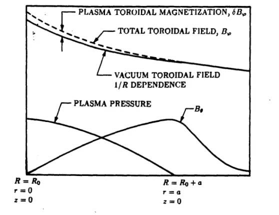
PLASMA TOROIDAL MAGNETIZATION, 6B,

TOTAL TOROIDAL FIELD, B,

VACUUM TOROIDAL FIELD 1/RDEPENDENCE

PLASMA PRESSURE

R=O _{R = Ro +a}

r=0 _{r a}

z=0 z=0

Figure 1.3.4. Magnetic field and pressure profiles in a tokamak. This figure shows the minor radial variation of the pressure and magnetic field in a typical tokamak equilibrium. The plasma pressure is assumed to be peaked in the center. The plasma current is also peaked at the center, so that Be is concave downward inside the plasma. Outside.the plasma, Bo has a predominantly 1/r dependence. Since the plasma is confined mainly by the poloidal field, Bw is only slightly different from the vacuum field, as evidenced by the smallness of 6B,. The fact that the net plasma toroidal magnetization is positive indicates that the flux due to the force-free current is usually slightly greater than the diamagnetic flux. Inspection of Eq. (2.3.11) indicates that bB, positive implies 6p less than 1, which is typical for a tokamak equilibrium.

Then, since the confining field is Be, it follows that the pressure scales according to

These relations, in addition to e < 1, are exploited in the analyses in Chapters 2 and 3.

To relate these fields and currents to the concept of plasma diamagnetism, it is helpful to imagine the current density resolved into components parallel and per-pendicular to the resultant helical magnetic field. Eq. (1.3.6) indicates that the resultant field points primarily in the toroidal direction. Eq. (1.3.7) indicates that the angle between J and B is very small. Eq. (1.1.1) indicates that only the compo-nent of J perpendicular to B contributes to plasma confinement, or, alternatively,

the diamagnetic drift current is a helical current flowing perpendicular to the mag-netic field lines, which, .according to Eq. (1.3.7), is smaller than the total current density by a factor of f2_{. On any given flux surface, this diamagnetic drift current}

can be thought of as forming a "solenoid" which, according to the right-hand rule, produces a magnetization that always opposes the toroidal field. The component of J parallel to B does not contribute to confinement and is therefore called the force-free current. On any given flux surface, this current forms a "solenoid" which produces a toroidal magnetization that always adds to the toroidal field. Even though the diamagnetic drift current is much smaller than the force-free current, the helicity of the force-free current is smaller than that of the diamagnetic drift current by e2 so that their toroidal magnetic fluxes are of comparable magnitudes. Thus the net plasma toroidal magnetization flux is a quantity of order E2 _{or perhaps}

even e3 _{which in practice can be very difficult to measure with precision.}

It is important to observe that the sense of the toroidal field in relation to that of the plasma current does not alter these relations. Fig. 1.3.3a shows the case where the plasma current is driven in the same direction as the toroidal field. The direction of the plasma current determines the sense of the helicity of the total magnetic field. Since the force-free current must flow along these lines, it then follows that the toroidal flux due to this current must add. to the applied toroidal field. Then, since the sense of the helicity of the diamagnetic drift current is opposite that of the force-free current, the toroidal flux due to the diamagnetic drift current must oppose the applied toroidal field. Fig. 1.3.3b shows the case where the plasma current is driven in the other direction. This causes the helicity of the force-free current to reverse. However, since the current is also driven in the opposite direction toroidally, the net effect is that the toroidal flux due to the force-free current still adds to the applied toroidal field. Also note that, while the sense of the helicity of the diamagnetic drift current is also reversed, it too must reverse direction in order that Eq. (1.1.1) be satisfied. This effect can be exploited to measure the extraneous linkage of the plasma current by the diamagnetic loops, as discussed in Chapter 4. At this point it is possible to predict the form of the expression for the toroidal flux due to plasma magnetism. Since the helicity of the "solenoid" foirmed by the force-free current is directly proportional to the magnitude of the plasma current, it follows that the toroidal flux should be proportional to the square of the plasma current. This is consistent with the observation that the sign of the force-free toroidal flux does not reverse when the plasma current is reversed. According to the simple models in Section 1.2, the toroidal flux due to plasma diamagnetism should

be in the opposite direction and should be directly proportional to the volume average of the plasma pressure. Based on these considerations, the expression for the toroidal flux'due to plasma magnetism should be of the form

A oc AJ 2 _{- C (p) (1.3.8)}

where A and C are constants and

()

Note that there are two subtractions called for in the diamagnetic measurement. The A in the expression for At indicates that the vacuum field must be subtracted from the total field to obtain the plasma magnetism. Physically, this is done by subtracting the rogowski coil signal from the diamagnetic loop signal at the input of the instrumentation circuit. The subtraction indicated on the right hand side of Eq. (1.3.8) indicates that the field due to the force-free current must be subtracted from the plasma magnetism to obtain the plasma diamagnetism. Since this -term involves the square of the plasma current, it is more convenient to implement this subtraction digitally, during data processing. The alternative would be to attempt

to construct an analog squaring circuit. The signal for the plasma current is ob-tained from a conventional rogowski coil installed on the vacuum chamber of the tokamak.

1.4 MHD Model of Plasma Equilibrium

In the ideal MHD description, the plasma is modeled as a perfectly conducting fluid. The equations describing the behavior of such a fluid in the presence of electric and magnetic fields are as follows:

ap -- + V -pv = 0 (1.4.1) at dv p- = J x B - Vp (1.4.2) dt ~(p/p') = 0 (1.4.3) E + v x B = 0 (1.4.4) B t x(1.4.5) V x B =J (1.4.6)

p is the mass density of the fluid, v is the fluid velocity, p is the kinetic pressure of the fluid, -y is the ratio of specific heats, and J, B, and E are the usual electromagnetic field quantities. A derivation of these equations starting from the equations of kinetic theory can be found in the review article by Freidberg [2].

The validity of these equations is not easy to establish. Freidberg shows that the validity of these equations requires three conditions: (1) the ion gyroradius must be small compared to the macroscopic scale length; (2) the plasma must be sufficiently large and collision-free that resistive diffusion is negligible; and (3) the plasma must be sufficiently collisional that the pressure is isotropic, heat conduction along the field is small, and electron and ion temperatures are equilibrated. In plasmas of fusion interest, such as in Alcator C, the third condition is usually not satisfied. However, it can be shown that the predictions of ideal MHD are approximately correct if variations along the magnetic field lines are sufficiently small. In particular, the analysis of Chapter 3 concerning anisotropic pressure will not be valid if the anisotropy is too large. In practice, the validity of these equations is usually justified on the grounds that their predictions agree well with experiment. In this paper, I will be concerned with plasma equilibrium involving no fluid flow. In this case, I set d/dt, 8/Ot, and v equal to zero in the MHD equations. Then Eqs. (1.4.1) and (1.4.3) reduce to 0 = 0. Eq. (1.4.4) then reduces to E = 0 and then Eq. (1.4.5) becomes 0 = 0. The description for flowless equilibrium then reduces to the following:

J X B = Vp (1.4.8)

V x B = J (1.4.9)

V -B = 0 (1.4.10)

The equation of state (Eq. (1.4.3)) will then be replaced by the ideal gas law

p = nT (1.4.11)

where n is the sum of the densities of all charged particle species present and p is the total kinetic pressure. Strictly speaking, condition (3) above requires that T be the same for all species, but since the model is to be used even when this is not exactly correct, the equation of state may also be generalized to

P= njT .(1.4.12)

where j is the species index.

19

(1.4.7) V -B = 0

CHAPTER 2: The Grad-Shafranov Equation for Plasma Equilibriumn

2.1 Derivationiof the Grad-Shafranov Equation

In the ideal magnetohydrodynamic (MHD) description of plasma equilibrium, the plasma is modeled as a perfectly conducting fluid. The pressure balance equa-tion,

Vp = J x B, (2.1.1)

describes the balance between kinetic pressure (assumed isotropic) and the Lorentz force. J and B must satisfy Ampere's law,

V x B = J, (2.1.2)

Gauss' law,

V B =0, (2.1.3)

and conservation of charge,

V -J =0. (2.1.4)

In these equations, all time derivatives, fluid velocities, and electric fields have been set to 0 to describe an equilibrium with no fluid flow.

In order to relate plasma diamagnetism to plasma pressure, one must imagine solving this system for p as a function of the magnetic field. This would involve substituting Eq. (2.1.2) into Eq. (2.1.1) and perhaps using Eqs. (2.1.3) and (2.1.4) for simplification. Then, since the measurement involves the total toroidal flux, there would be a surface integral over the plasma poloidal cross section. Such an analysis is carried out in Chapter 3 for the case of anisotropic plasma pressure. However, if the pressure is assumed to be isotropic and there are no variations in the toroidal' direction, then the entire system of vector equations can be reduced to a single partial differential equation in a single unknown - the Grad-Shafranov equation. In either case, the solution involves two unspecified functions that are related to plasma pressure and current profiles. These profiles cannot be predicted from ideal MHD theory. If an analysis of them was to be carried out, one would have to use a kinetic model of the plasma.

One of the unspecified functions will be denoted by p and is the plasma pres-sure profile, and thus is related to the distribution of thermal energy in the plasma. The other function will be denoted by F and describes the distribution of cur-rent within the plasma. Thus F is related to the plasma diamagnetism while p

is related to the plasma thermal energy. The Grad-Shafranov equation is there-fore the desired relation between diamagnetism and thermal energy. Of course the Grad-Shafranov equation will also contain other information, since it relates all the magnetic fields and currents in the plasma - not just those having. to do with the diamagnetic measurements. The single scalar function that satisfies the Grad-Shafranov equation will be the poloidal magnetic flux associated with a particular point in the poloidal plane, that point being located in the two-dimensional domain of the Grad-Shafranov equation.

The derivation of the Grad-Shafranov equation exploits the assumed isotropy of the pressure and the axisymmetry of the tokamak. Since the tokamak is symmetric about the major axis, the toroidal angular coordinate p is an ignorable coordinate. From the theory of vector calculus, it is known that a divergenceless vector field can be expressed as the curl of some other vector. Also, if there is an ignorable co-ordinate and the divergenceless vector has no component in the ignorable direction, then the divergenceless vector can be expressed in terms of a single scalar quantity called a stream function [6]. In the present analysis, the magnetic field is diver-genceless, but it does have a component in the ignorable (p) direction. Therefore, while the toroidal field will be retained as one scalar variable, the poloidal field will be reduced to one scalar stream function, which will turn out to be the poloidal flux. The remaining toroidal field will contain a known (applied) vacuum contribution (zero order in E), and contributions which are related to p and F. In addition, the stream function will also be related to p and F.

To obtain the desired relation between plasma diamagnetism and thermal en-ergy, only the zero order solution of the Grad-Shafranov equation is required. The resulting solution is usually expressed in terms of a dimensionless quantity called the poloidal beta and denoted by 6p. The poloidal beta can be defined as the ra-tio between the volume averaged plasma pressure and the magnetic stress at the plasma surface due to the poloidal field. This quantity (0p) also appears in equa-tions describing the major radial equilibrium of the plasma from which one can obtain a measure of the magnetic energy stored in the force-free plasma current [13],[14]. Since these equaticns come from the first order solution of the Grad-Shafranov equation, some analysis related to them is also included. In particular the effect of pressure anisotropy appears differently in the first order solution and it is important to note this difference. A few higher order expressions are included only for completeness, in that they comprise the first occurances of contributions from all terms in the full Grad-Shafranov equation.

The following derivation of the Grad-Shafranov equation closely follows that given by Freidberg [3]. The coordinate systems for the following analysis are illus-trated in Fig. 1.3.1. Since V -B = 0, the magnetic field can be written in terms of the vector potential: B = V x A. Since there is no variation in the toroidal direction, the poloidal magnetic field can be written in terms of a scalar stream function. In cylindrical (R, p, z) coordinates, the curl of a vector is given by

V - 3aA 1 aAo .OAR A 1 a 1OARJ

V x A = + O +i (RAw) - -_

R dz + &c z dR RaR R p

(2.1.5) Since there is no variation in the p-direction, this reduces to

aAR aA, BP =9 (2.1.6) and Bp = -- AW+ R- (RA.) (2.1.7) or 1 89 13 B, = - R (RA,)+ - (RAw). (2.1.8) R az R aR

Therefore, the magnetic field can be expressed in terms of two scalar quantities: the toroidal magnetic field B,,, and the stream function 0, where

R Ap. (2.1.9)

B =A ( z )+ OB + R 1R (2.1.10)

Next, using

VxB=J, _(2.1.11)

the current density can be written in terms of the same two quantities as

= 1 1

J = 1 l * O + 1-V(RBV) x 0, (2.1.12)

R R

where the differential operator A* is defined by

a

The next step is to substitute these quantities into Eq. (2.1.1). The easiest way to do this is to resolye Eq. (2.1.1) into components along B, along J, and along Vik. The component along B yields

B - Vp = B -J x B = 0. (2.1.14)

This means that the pressure does not vary on a magnetic flux surface. Therefore, the pressure can be expressed as a function of the single variable i.

p = p(#) (2.1.15)

The pressure gradient is therefore given by

Vp = dVP. (2.1.16)

dik The component along J yields

J - Vp 0 (2.1.17)

which can be combined with Eq. (2.1.12) to yield

0 = [ V(RB,) x - V . (2.1.18)

.R I dO$

This means that the scalar function RB, F is also a function of the single variable so that

RB, = F(P) (2.1.19)

and

VF = dFV. (2.1.20)

dO

Physically, this means that electric current flows along magnetic flux surfaces, or equivalently that magnetic flux surfaces are also electric current flux surfaces. Note also that the quantity -F represents the poloidal current flux and is a stream function for the poloidal current.

Finally, by using these results and taking the component of Eq. (2.1.1) along VO one obtains

2d p d F

-- M*k = R + F--. (2.1.21)

which is the Grad-Shafranov equation. This equation gives the flux function,

k,

2.2 Asymptotic Expansion of the Grad-Shafranov Equation

The operator A* can be written in toroidal (r, p, 0) coordinates as

.1

a ao

1 a20

1

sin 0

*.-r- +-

(

+r r88 R ar r 8 so that the Grad-Shafranov equation becomes

1

a ao

ai

--- r- + cos

6

F d.

78 87 r --

Ro

The problem now is how to solve this equation. This is an inhomogeneous, partial differential equation. In addition, since the forcing functions p and F are functions of the dependent variable 0, it is also nonlinear. However, it will turn out to be possible to obtain a useful solution to this equation by making an assumption about the shape of the plasma and exploiting the smallness of the inverse aspect ratio by means of an asymptotic expansion (which turns out to be a regular perturbation series). Since the vacuum vessel and limiters in the Alcator C tokamak are circular, the plasma will be assumed to form circular flux surfaces at initial breakdown. Since the plasma position in Alcator C is maintained by a vertical field with no significant quadrupole component, it can be shown that the flux surfaces will tend to remain circular as the discharge evolves [101. Thus, the plasma will be assumed to be circular to zero order in c. Also as E tends to zero and a remains finite, RO must become infinite, so that the toroidal shape of the plasma becomes an infinite circular cylinder. It then follows from symmetry that the flux surfaces must

be concentric cylinders, and that the stream function depends only on r. Thus

the zero order solution to the Grad-Shafranov equation will be only a function of the minor radial coordinate. This reduces the zero order equation to an ordinary

differential equation.

The inverse aspect ratio, f, of the torus is given by

f =_ -

<

Ro

For a tokamak, the magnetic field and pressure scale according to

(2.2.5) and

6B, ~ c2_{BW (2.2.6)}

where 6B is the plasma toroidal magnetization. These relations can be made explicit by defining all quantities in terms of new, dimensionless quantities, scaled so that all dimensionless quantities are of order 1. This is done in the following definitions.

r ax, therefore 0 < r < a -+ 0< x < 1 (2.2.7)

R Roy(X, 0), y = 1 + EXcosO (2.2.8)

= RAO = (Roy)(EaBoa) (2.2.9)

f ya = dimensionless stream function (2.2.10)

p 2 .BoP (2.2.11)

F =RBW = RBp0 + RbB, = ROBo + RbBp M RoBo + RoyBo 2g (2.2.12) = RoBo(l + E2 _yg)

i = yg = dimensionless poloidal magnetization current (2.2.13) This results in the following dimensionless Grad-Shafranov equation:

1

a

Of

a

2dP 2 di

-- + - cos# - y

(1+E

X X aX x2 902 y Ox

X

Note that the problem is regular in E so that a solution in terms of a series with nonzero radius of convergence is expected. The new dimensionless quantities are summarized below:

x = minor radial coordinate = r/a (2.2.15)

f = ya = poloidal flux = 0/(aERoBo) (2.2.16)

E = inverse aspect ratio = a/Ro (2.2.17)

y = major radial coordinate = R/RO = 1 + Ex cosB (2.2.18) p~, Bi ~ E2 B 2

e

P = kinetic pressure = p/ B) (2.2.20)

i = yg = poloidal magnetization current = RBQ,/(E2 RoBo) (2.2.21) a = toroidal component of vector potential = A,/(EaBo) (2.2.22)

g = plasma diamagnetism = 6B/(E2_{Bo) (2.2.23)}

It is also helpful to define a dimensionless magnetic field:

b _{rb, + 6b, + Ob,}

E2BO eB0 Bo (2.2.24)

(

1

af

1)

_{+b l f}

-X'

The solution will be expressed in terms of a regular perturbation series in E:

f(X, e) ~ fo(X) + efi(X, 0) + E2f2

(z,O

y = 1 + Ezcoso (2.2.26)

y2 = 1 + E2x cos 0 + E 2x 2 cos2_o

(2.2.27)

1/y~_1-ExcosB+E 2_X2_cos2 _{o+... (2.2.28)}

and the flux functions are Taylor expanded about the zero order solutions:

P(f) ~ P(fo) + EfiP'(fo) + E2

(f

i(f) i(fo) + Efi'(fo) +

ffo)

i'(f) ~ i'(fo) + Efii"(fo) + 6E 2 fi + )

Substitutingtall these expansions into the Grad-Shafranov equation and retain-ing terms to second order in E yields

1a

a

1

a2

yo + EfI E+ 2f2) + 2 2(e!1+ 2f2)

- E(1-

xcos)cos

_{(fo +}

₊

= -(1+ E2xcosO + 622 2 9) P, + EfIP" + E2 f +

- (1+ 62_i)

[i'

Sf + f2 ) ' ].

(2.2.33) Collecting powers of e yields

1(

+ f

X

I

+E2 a af2

1 _a2_f,

2 a192 - cos 8 _OxJI

+ 2 -cas +XCOS2 a + 1sin8 I

x OxJ

= -(P + i') - 6(fiP" + 2xcosOP' + fi")

+ f2 P"'+ 2xcos Of1P" + x2 Cos+2 P + f2)' + ii']

(2.2.34)

from which the perturbation equations can be read off. The zero-order equation is

1 d dfo d

=

x dx (P + i), (2.2.35)

the first order equation is

dfo - cos-dx dP - 2xcos- -dfo d 2 f- f---(P +), d0o and the second order equation is

1- 0 0fM Xx OIx

9

(cos

_-

x

ax

f

The tangential magnetic field

a f

ybe = -- (2.2.38)

ax

can be expanded to yield

dfo

-- = boo, (2.2.39)

= _{beI + x cos 0 bo, (2.2.40)}

ax

and

- = b 2 + x cos 0 be. (2.2.41)

ax

And the radial magnetic field

Exyb,. = (2.2.42)

ae

can be expanded to yield

8fi

= -xb,.o, (2.2.43)

and,

af

2

2.3 Zero Order Solution of the Grad-Shafranov Equation

To obtain the desired relation between toroidal magnetization flux and plasma pressure, it has already been anticipated that an integration over the poloidal cross-section will be called for. In preparation for this, it is helpful to first eliminate the dependent poloidal flux variable in favor of the -component of the magnetic field. The zero-order equation can be written as

1 d dfo dx d

- -- + (P + i) = 0. (2.3.1)

Xdx dx dfodX

Use of Eq. (2.2.39) enables this to be written as

b 2 _--

_0-

-20 + p + i) = 0. (2.3.2)

x dx2

This equation is the radial pressure balance equation for the tokamak. It is a relation between the three quantities P, i, and be. P is the plasma pressure and i is a measure of the plasma diamagnetism, while be is a third quantity which to

zero order is a measure of the plasma current. The radial pressure balance equation can be solved for .the plasma toroidal magnetization flux in terms of the spatially averaged kinetic pressure and the plasma toroidal current by multiplying by x (an integrating factor), and integrating over the poloidal cross-section of the plasma column. Since there is no p-variation, the spatial average of a quantity q becomes

(q(x, 0)) = q(x,O)dA = 3 -j, O)f dx d . (2.3.3)

For a quantity that has only radial variation, this reduces to

(q(x)) = 21 q(x)x dx. (2.3.4)

After multiplying Eq. (2.3.2) by x and integrating each term over the poloidal cross-section, one obtains

[boo(x = 1)] 2 _{- (P) -2 ixdx= 0.}

(2.3.5)

The first term is a boundary term, where bgo(x = 1) represents the poloidal magnetic field at the plasma surface. (The radial component is zero because the plasma surface is a flux surface.) The remaining integral can be rewritten as

2/f1 2ixd=- ygxdx d

0 -0 0

1f27r f1 _{2v 12(-36}

Sj _{g(x, ) x dx dO + g(x,)2 cosOdxdO (2.3.6)}

1

where the second integral on the second line is identically zero if the plasma magne-tization is assumed to be symmetric about the line y = 1. (More will be said about this assumption in Section 2.5.) 64 represents the plasma toroidal magnetization and is given by

64

g

where

AP= 2f aBwr dr d (2.3.8)

is the plasma magnetization in MKS units. Using the result of Eq. (2.3.6) in Eq. (2.3.5) yields.

1 1

(P) = - Ibeo(1)]2 - -bo (2.3.9)

2 7

Note that, since beo(1) is directly proportional to the plasma current, this expression agrees with the prediction made in Eq. (1.3.8).

The poloidal beta, #p is now defined as the ratio of the spatially averaged kinetic pressure (or perpendicular kinetic energy) to the poloidal field energy at the plasma surface:

(F) (p)

)= .[BP)(P) (2.3.10)

[ boo(1)] 2 Bo(a) ]2

The last expression is the definition in MKS, units. The final result is that the radial pressure balance is described by the equation

= _ 264 82rBo M

OP = 1

[bo

7r [boo(l)| y 52

where the MKS expression comes from the zero-order approximation

Beo(a) = A (2.3.12)

27ra

and I is the plasma current.

2.4 First Order Solution of the Grad-Shafranov Equation

The first-order equation is

1a '9fi 1 a2f, dfo dP d2

--X + = cos-- - 2x cos6- - fi -- (P + i). (2.4.1)

X (x C : X2 502 dx dfo dfo

Assuming that the zero-order solution fo is known, the first-order equation is now linear (but inhomogeneous). It is also separable. The substitution

fi(,9) = u(X)t(o) (2.4.2)

yields

t(0)

z-X + -2---u()- (P + ). (2.4.3)

Since the first two terms on the right-hand side are independent of 0, every other term must also be independent of 0, which requires

t oc cos 6 and t" oc cos 0.

Choosing t = cos 0 yields the following ordinary differential equation:

dfo dP dx dfo d2 - (P + ) df Using dfo

dx

beo,

f-

this can be written as

boo d du b2 dP

x

[b90

U [bo- d 1 d

dx boo d9 (2.4.7)

After substituting the zero-order result

2

(P + i) - - (2.4.8)

(from Eq. (2.3.2)) and performing some manipulation, this can be written as d 2 d

24 dP

Tx[bo* dz \ue x b -2x2 (2.4.9)

One integration then yields

boo 2x2 (P) + U ) =] or d dx (u 'b8O) (P) - P Ib2 2 0

After defining a dimensionless local internal inductance,

-(bj ₀)=

1i

-(

1 (09).

and a local poloidal beta,

(P) - P(X) (

OP = b 0 O3P(x), (2-4.13)

and performing a second integration, the first-order solution is obtained:

f, = beo(x) cos 0 1'(p (t) + t dt (2.4.14)

This first order solution is concerned with the major radial equilibrium of the plasma, as discussed by Pribyl [14] and Pickrell 113]. The plasma has a tendency to expand in the major radial direction which can be counteracted by the application of a vertical field which interacts with the plasma toroidal current. The intensity of the required vertical field depends on the quantity fi and hence is a measure of the quantity 3_{p + li/2. In principle the measurement of the required vertical} field can be combined with the diamagnetic measurement to obtain a measure of li/2. In the case of isotropic plasma pressure the poloidal beta used in the vertical field measurement is related to the poloidal beta in the diamagnetic measurement

by #p(1) = #p from the diamagnetic measurement. However, as pointed out in

Chapter 3, the relationship is more complicated in the case of anisotropic pressure. In that case, the poloidal beta from the diamagnetic measurement is influenced only by the perpendicular pressure while the poloidal beta in the vertical field measurement is influenced by both the perpendicular and parallel pressure.

2.5 Higher Order Corrections to the Poloidal Beta

In Alcator C the value of E is 1/4, which is a typical value for the inverse aspect ratio of a tokamak. While this value is sufficiently small that one can be reasonably confident that the perturbation series is convergent, it is also sufficiently large that one should be worried about the accuracy of a measurement that contains no higher order corrections. Actually, it is easy to show that the higher order corrections to

the poloidal beta are small enough to be neglected.

There are two places in the analysis where approximations have been made and where corrections have to be investigated. First, consider Eqs. (2.2.29) and (2.2.30) which are the asymptotic expansions of the plasma pressure and magnetization, respectively. Mathematically, what was done to obtain Eq: (2.3.11) for the poloidal beta was to truncate these expansions after the first term and then integrate over the poloidal cross-section. Now consider the effect of including a first order term,

such as EfiP'(fo) in the calculation. Since P'(fo) depends only on x and f,(x,O) =

u(x) cos 9 then it i§ clear.that these terms do not contribute when integrated over the poloidal cross-section. Therefore, the next order correction from these expansions is of order e2, which is a reasonably small number.

The other approximation that was made occurred in Eq. (2.3.6), where the second integral on the second line was zero because the plasma magnetization was assumed to be symmetric about the line y = 1. The asymmetry about this line will be due to the Shafranov shift [2j,[3j,[10],[12],[13],[14]. Since the Shafranov shift is first order in e, and since g is proportional to )3_{p, this correction is of order}

E2 ,Ip and therefore is also reasonably small.

These corrections were calculated numerically for a typical plasma by Shafranov [18].

CHAPTER 3: Tensor Representation of Plasma Equilibrium

3.1 Derivation of the Total Pressure Tensor

In this chapter, I will consider the case of a plasma with anisotropic kinetic pressure. In this case, the formalism of the Grad-Shafranov equation is not very helpful and a more direct approach by means of a total pressure tensor is more appropriate. In this case, the pressure balance equation becomes

V -=JxB (3.1.1)

where B and J still satisfy Ampere's law

VxB=J (3.1.2)

and Gauss' law

V B .= 0. (3.1.3)

At any point in the plasma, the pressure in the direction of the magnetic field will be different than the pressure perpendicular to the magnetic field. Therefore, in a coordinate system in which the magnetic field lines lie along the third coordinate curves (e.g. flux coordinates), the kinetic pressure tensor will be given by

pj- 0 0

S= 0 P-L 0 .(3.1.4)

0 0 P11 By transforming to a coordinate system in which

B = 83B = i1 B1 + 2B2 + k3B3, (3.1.5) _B 83 = B (3.1.6) B and 61 X 82 = 63, (3.1.7)

this can be written more generally as

or

BB

. . = pJ+(p 1 - p)- , (3.1.9)

where I is the identity matrix.

By combining the pressure balance equation with Ampere's law and Gauss' law, the equilibrium condition can be written in terms of a total pressure tensor, which is the sum of the kinetic pressure tensor and the magnetic stress tensor. To do this, Eq. (3.1.1) is combined with Eq. (3.1.2) to obtain

V.+Bx(VxB)=0. (3.1.10)

The cross product can then be written as the divergence of a tensor by applying some vector identities and using Gauss' law as follows:

B x (V x B) =

jV(B

= V - (-jB21) - V (BB) + B(V - B) (3.1.11)

= V -(B2I - BB).

Thus, the equilibrium condition can be written as

V -t = 0, (3.1.12)

where t is the total pressure tensor, and is given by

2

= B2_{1 - BB. (3.1.13)}

The elements of I are

tij = tj bi - B2 _{+ tiB (3.1.14)}

where

t = p + B2(3.1.15)

and