HAL Id: hal-02123389
https://hal.archives-ouvertes.fr/hal-02123389
Submitted on 21 Aug 2020
HAL is a multi-disciplinary open access
archive for the deposit and dissemination of
sci-entific research documents, whether they are
pub-lished or not. The documents may come from
teaching and research institutions in France or
abroad, or from public or private research centers.
L’archive ouverte pluridisciplinaire HAL, est
destinée au dépôt et à la diffusion de documents
scientifiques de niveau recherche, publiés ou non,
émanant des établissements d’enseignement et de
recherche français ou étrangers, des laboratoires
publics ou privés.
Peak star formation efficiency and no missing baryons in
massive spirals
Lorenzo Posti, Filippo Fraternali, Antonino Marasco
To cite this version:
Lorenzo Posti, Filippo Fraternali, Antonino Marasco. Peak star formation efficiency and no missing
baryons in massive spirals. Astron.Astrophys., 2019, 626, pp.A56. �10.1051/0004-6361/201935553�.
�hal-02123389�
https://doi.org/10.1051/0004-6361/201935553 c L. Posti et al. 2019
Astronomy
&
Astrophysics
Peak star formation efficiency and no missing baryons
in massive spirals
Lorenzo Posti
1,2, Filippo Fraternali
1, and Antonino Marasco
1,31 Kapteyn Astronomical Institute, University of Groningen, PO Box 800, 9700 AV Groningen, The Netherlands 2 Université de Strasbourg, CNRS UMR 7550, Observatoire astronomique de Strasbourg, 11 rue de l’Université,
67000 Strasbourg, France
e-mail: [email protected]
3 ASTRON, Netherlands Institute for Radio Astronomy, Oude Hoogeveensedijk 4, 7991 PD Dwingeloo, The Netherlands Received 26 March 2019/ Accepted 30 April 2019
ABSTRACT
It is commonly believed that galaxies use, throughout Hubble time, a very small fraction of the baryons associated with their dark matter halos to form stars. This so-called low star formation efficiency f? ≡ M?/ fbMhalo, where fb ≡ Ωb/Ωcis the cosmological baryon fraction, is expected to reach its peak at nearly L∗
(at efficiency ≈20%) and decline steeply at lower and higher masses. We have tested this using a sample of nearby star-forming galaxies, from dwarfs (M? ' 107M ) to high-mass spirals (M? ' 1011M ) with Hi rotation curves and 3.6 µm photometry. We fit the observed rotation curves with a Bayesian approach by varying three parameters, stellar mass-to-light ratioΥ?, halo concentration c, and mass Mhalo. We found two surprising results: (1) the star formation efficiency is a monotonically increasing function of M?with no sign of a decline at high masses, and (2) the most massive spirals (M? ' 1−3 × 10¹¹M ) have f? ≈ 0.3−1, i.e. they have turned nearly all the baryons associated with their halos into stars. These results imply that the most efficient galaxies at forming stars are massive spirals (not L∗galaxies); they reach nearly 100% efficiency, and thus once both their cold and hot gas is considered in the baryon budget, they have virtually no missing baryons. Moreover, there is no evidence of mass quenching of the star formation occurring in galaxies up to halo masses of a few × 1012M
.
Key words. galaxies: kinematics and dynamics – galaxies: spiral – galaxies: structure – galaxies: formation
1. Introduction
In our Universe, only about one-sixth of the total matter is baryonic, while the rest is widely thought to be in form of non-baryonic, collisionless, non-relativistic dark matter (e.g.
Planck Collaboration VI 2018). In the so-called standardΛ cold dark matter (ΛCDM) paradigm, galaxies form within extended halos of dark matter that were able to grow enough to become gravitationally bound (e.g.White & Rees 1978). In this scenario it is then reasonable to expect that the amount of baryons present in galaxies today is roughly a fraction fb ≡ Ωb/Ωc = 0.188
(the cosmological baryon fraction; e.g.Planck Collaboration VI 2018) of the mass in dark matter. However, it was realised that the total amount of baryons that we can directly observe in galax-ies (stars, gas, dust, etc.) is instead at most only about 20% of the cosmological value (e.g.Persic & Salucci 1992;Fukugita et al. 1998). This became known as the missing baryons problem and has prompted the search for large resevoirs of baryons within the diffuse, multi-phase circumgalactic medium of galax-ies (Bregman 2007;Tumlinson et al. 2017).
Arguably the most important indicator of this issue is the stellar-to-halo mass relation, which connects the stellar mass M? of a galaxy to its dark matter halo of mass Mhalo (see Wechsler & Tinker 2018, for a recent review). This relation can be probed observationally through many different tech-niques, e.g. galaxy abundance as a function of stellar mass (e.g.
Vale & Ostriker 2004;Behroozi et al. 2010;Moster et al. 2013), galaxy clustering (e.g.Kravtsov et al. 2004;Zheng et al. 2007), group catalogues (e.g. Yang et al. 2008), weak galaxy-galaxy
lensing (e.g. Mandelbaum et al. 2006; Leauthaud et al. 2012), satellite kinematics (e.g.van den Bosch et al. 2004;More et al. 2011; Wojtak & Mamon 2013), and internal galaxy dynamics (e.g. Persic et al. 1996; McConnachie 2012; Cappellari et al. 2013;Desmond & Wechsler 2015;Read et al. 2017;Katz et al. 2017; hereafter K17). Amongst all these determinations there is wide consensus on the overall shape of the relation and, in particular, on the fact that the ratio of stellar-to-halo mass f? = M?/ fbMhalo(sometimes called star formation efficiency),
is a non-monotonic function of mass with a peak ( f? ≈ 0.2)
at Mhalo ≈ 1012M (roughly the mass of the Milky Way). One
interpretation is that galaxies of this characteristic mass have been, during the course of their lives, the most efficient at turning gas into stars. Even so, efficiencies of the order of 20% are still relatively low, implying that most baryons are still undetected even in these systems1.
Several works have suggested that the exact shape of the stellar-to-halo mass relation depends on galaxy morphology (e.g.
Mandelbaum et al. 2006;Conroy et al. 2007;Dutton et al. 2010;
More et al. 2011; Rodríguez-Puebla et al. 2015; Lange et al. 2018), especially on the high-mass side (log M?/M & 10)
where red, passive early-type systems appear to reside in more massive halos with respect to blue, star-forming, late-type galax-ies. This is intriguing since it suggests that galaxies with different morphologies likely followed different evolutionary pathways that led the late-type ones, at a given M?, to live in lighter halos
1 Since molecular, atomic, and ionised gas is typically dynamically sub-dominant in M?> 1010M galaxies.
Open Access article,published by EDP Sciences, under the terms of the Creative Commons Attribution License (http://creativecommons.org/licenses/by/4.0),
A&A 626, A56 (2019)
and to have a somewhat smaller fraction of missing baryons with respect to early-type systems2. However, one of the main
difficulties associated with these measurements is the scarcity of high-mass galaxies in the nearby Universe (e.g.Kelvin et al. 2014), given that most of the above-mentioned observational probes use statistical estimates based on large galaxy samples.
In this paper we use another, complementary approach to estimate the stellar-to-halo mass relation through accurate mod-elling of the gas dynamics within spiral galaxies. We use the observed Hi rotation curves of a sample of regularly rotating, nearby disc galaxies to fit mass models comprising a baryonic plus a dark matter component. We then extrapolate the dark mat-ter profile to the virial radius, with cosmologically motivated assumptions, to yield the halo mass. A considerable advantage of this method is that each system can be studied individually and halo masses, along with their associated uncertainties, can be determined in great detail for each object. We show that this approach leads to a coherent picture of the relation between stel-lar and halo mass in late-type galaxies, which in turn profoundly affects our perspective on the star formation efficiency in the high-mass regime.
The paper is organised as follows: we present our sample and methodology to derive stellar and halo masses in Sect.2; we describe our results in Sect.3; and we discuss the results in detail in Sect.4.
2. Method
Here we describe the data and methodology of our analysis. We adopt a standardΛCDM cosmology with parameters estimated by thePlanck Collaboration VI (2018). In particular, we use a Hubble constant of H0 = 67.66 km s−1Mpc−1and a
cosmologi-cal baryon fraction of fb ≡Ωb/Ωc= 0.188.
2.1. Data
We use the sample of 175 disc galaxies with near-infrared pho-tometry and Hi rotation curves (SPARC) collected byLelli et al.
(2016a; hereafter LMS16). This sample of spirals in the nearby Universe spans more than 4 orders of magnitude in luminos-ity at 3.6 µm and all morphological types, from irregulars to lenticulars. The galaxies were selected to have extended, regular, high-quality Hi rotation curves and measured near-infrared pho-tometry; thus, it is not volume limited. Nevertheless, it still provides a fair representation of the population of (regularly rotating) spirals at z = 0 and most importantly is best suited for our dynamical study.
The Hi rotation curves are used as tracers of the circular velocity of the galaxies, while the individual contributions of the atomic gas (Vgas) and stars (V?) to the circular velocity are
derived from the Hi and 3.6 µm total intensity maps, respec-tively (see LMS16, for further details). The velocity Vgastraces
the distribution of atomic hydrogen, corrected for the presence of helium, while the near-infrared surface brightness is decom-posed into an exponential disc (Vdisc) and a spherical bulge
(Vbulge). The contribution of the stars to the circular velocity is
then V2
? = ΥdiscVdisc2 + ΥbulgeVbulge2 , given stellar mass-to-light
ratios of the disc (Υdisc) and bulge populations (Υbulge).
2 Blue galaxies typically also have larger reservoirs of cold gas with respect to red ones. However, on average, the amount cold gas is sub-dominant with respect to stars for M?> 1010M . (e.g.Papastergis et al.
2012).
2.2. Model
We model the observed rotation curve as Vc=
q
VDM2 + Vgas2 + V?2. (1)
Here VDM is the dark matter contribution to the
circu-lar velocity; for simplicity, we have assumed that Υbulge=
1.4Υdisc, as suggested by stellar population synthesis
mod-els (e.g. Schombert & McGaugh 2014), thus V?2= Υdisc(Vdisc2 +
1.4Vbulge2 ). In AppendixA we explore the effect of fixing
dif-ferent mass-to-light ratiosΥdisc and Υbulge for disc and bulge,
respectively: our findings on the stellar-to-halo mass relation do not change significantly if we assumeΥdisc= 0.5 and Υbulge= 0.7,
for which the scatter of the baryonic Tully–Fisher relation is minimised (Lelli et al. 2016b).
The dark matter distribution is modelled as a Navarro et al.
(1996; hereafter NFW) spherical halo, which is characterised by a dimensionless concentration parameter (c) and the halo mass (Mhalo), which we take as that within a radius enclosing
200 times the critical density of the Universe. Thus, our rotation curve model has three free parameters: Mhalo, c, andΥ?.
We compute the posterior distributions of these parameters with a Bayesian approach. We define a standard χ2likelihood P,
given the data θ, as χ2= − ln P(θ|M halo, c, Υdisc) = N X i=0 1 2
" Vobs,i− Vc(Ri|Mhalo, c, Υdisc)
σVobs,i
#2
, (2)
where Vobs,i is the ith point of the observed rotation curve at
radius Ri and σVobs,i is its observed uncertainty. The posterior distribution of the three parameters is then given by the Bayes theorem
P(Mhalo, c, Υdisc|θ) ∝ P(θ|Mhalo, c, Υdisc) P(Mhalo, c, Υdisc), (3)
where P(Mhalo, c, Υdisc) is the prior. We sample the posterior
with an affine-invariant Markov chain Monte Carlo method (MCMC, in particular, we use the python implementation by
Foreman-Mackey et al. 2013).
We use a flat prior on the stellar mass-to-light ratio Υdisc
limited to a reasonable range, 0.01 . Υdisc . 1.2, which
encompasses estimates obtained with stellar population models (Meidt et al. 2014;McGaugh & Schombert 2014). In a ΛCDM Universe the halo mass and concentration are well known to be anti-correlated. Thus, in order to test whether standardΛCDM halos can be used to fit galaxy rotation curves and then yield a stellar-to-halo mass relation, for the halo concentration we assume a prior that follows the c−Mhalorelation as estimated in
N-body cosmological simulations (e.g.Dutton & Macciò 2014; hereafter DM14): for each Mhalo, the prior on c is lognormal with
mean and uncertainty given by the c= c(Mhalo) of DM14 (their
Eq. (8)). The prior on the dark matter halo mass Mhalois, instead,
flat over a wide range: 6 ≤ log Mhalo/M ≤ 15.
A non-uniform prior on the halo concentration is needed to infer reasonable constraints on the halo parameters (see e.g. K17). The reason for this is that the Hi rotation curves do not typically extend enough to probe the region where the NFW den-sity profile steepens, thus yielding only a weak inference on c. The ΛCDM-motivated prior on the c−Mhalo relation proves to
be enough to constrain all the model parameters. Furthermore, we note that the DM14 c−Mhalo relation does not distinguish
between halos hosting late-type or early-type galaxies, so we use
Table 1. Priors of our model. P(Mhalo, c, Υ?) in Eq. (3) is given by the product of the three terms.
Parameter Type
Υ? Uniform 0.01 ≤Υ?≤ 1.2 Mhalo Uniform 6 ≤ log Mhalo/M ≤ 15
c Lognormal c−Mhalofrom DM14
it under the assumption that it provides a reasonable description of the correlation for the halos where late-type galaxies form. We summarise our choice of priors in Table1.
3. Results
We modelled the rotation curves and we measured the poste-rior distributions of Υdisc, Mhalo, and c for all the 158 SPARC
galaxies with inclination on the sky higher than 30◦ (for nearly
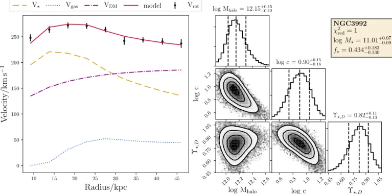
face-on systems the rotation curves are very uncertain). For each parameter, we define the best value to be the median of the poste-rior distribution and its uncertainty as the 16th–84th percentiles. In AppendixAwe provide all the measurements and uncertain-ties, together with the value of the likelihood associated with the best model (see TableA.1). We also present the full rotation curve decomposition for one case as an example (NGC 3992, Fig. A.1), while we make available the plots of all the other galaxies online3.
Unsurprisingly, we find that our model typically does not give very stringent constraints on the stellar mass-to-light ratio, with only 84 (68) galaxies having an uncertainty on Υ? lower than 50% (30%). In these cases, which are mostly for M? >
1010M
where the signal-to-noise ratio is high, the Vobsand V?
profiles are similar enough to yield good constraints onΥdisc. We
find that these galaxies are not all maximal discs, as theirΥdisc
is homogeneously distributed in the range allowed by our prior. We find the highest mass spirals (M?& 1011M ) to have much
better fits with a slightly higher mass-to-light ratio (Υdisc∼ 0.7)
than the mean of our prior (Υdisc = 0.6), consistently with
pre-vious works who found that high-mass discs are close to maxi-mum (e.g.Lapi et al. 2018;Starkman et al. 2018;Li et al. 2018). Smaller systems, instead, typically have a poorer inference on the mass-to-light ratio, with about ∼50 cases in which the pos-terior onΥdiscis quite flat. Even in these extreme cases it is still
useful to let the MCMC explore the full range of possible mass-to-light ratios (0.01 ≤ Υdisc ≤ 1.2) as opposed to just fixing a
value forΥdisc because it provides a more realistic estimate of
the uncertainty on the other parameters of the dark matter halo. In other words, when the inference on Υdisc is poor, it may be
thought of as a nuisance parameter over which the posterior dis-tributions of the other two more interesting halo parameters are marginalised.
For 137 galaxies (out of 158) we obtained a unimodal pos-terior distribution for the halo mass, thus we were able to asso-ciate a measurement and an uncertainty with Mhalo; instead, the
remaining 21 galaxies had either a multi-modal or a flat pos-terior on the halo mass and thus we discarded them. These 21 galaxies are mostly low-mass systems (M? . 2 × 10⁹M ) and
their removal does not alter in any way the high-mass end of the population, which is the main focus of our work. For some of the remaining 137 galaxies, we find that the NFW halo model
3 http://astro.u-strasbg.fr/~posti/PFM19_fiducial_ fits/ 109 1010 1011 1012 1013 Mhalo/M 107 108 109 1010 1011 1012 M? /M fbMhalo −1.00 −0.75 −0.50 −0.25 0.00 0.25 0.50 0.75 1.00 log MHI /M ?
Fig. 1.Stellar-to-halo mass relation for 110 galaxies in the SPARC sample. The points are colour-coded by the ratio of Hi-to-stellar mass. The stellar-to-halo mass relation estimated byMoster et al.(2013) using abundance matching is shown as a black dashed curve; the scatter of the relation is shown shaded in grey. Galaxies that have converted all the available baryons in the halo into stars would lie on the long-dashed line, whose thickness encompasses uncertainties on fb. For ref-erence, we also show the location of the Milky Way (cross) and of the Andromeda galaxy (plus) on the plot, as given by the modelling by
Posti & Helmi(2019) andCorbelli et al.(2010), respectively.
provides a poor fit to the observed rotation curve, as their best-fit χ2value is high. This is not surprising, since it is well known that
low-mass discs in particular tend to have slowly rising rotation curves, which makes them more compatible with having cen-trally cored halos (e.g.de Blok et al. 2001; K17). Indeed, by re-fitting all rotation curves with a cored halo model fromBurkert
(1995), we have found 27 mostly low-mass (M?. 1010M )
sys-tems for which a similar cored profile is preferred to the NFW at a 3-σ confidence level. For consistency we decided to remove these 27 systems from our sample, but in AppendixAwe demon-strate that their stellar and halo masses, derived by extrapolating the Burkert profile to the virial radius, are perfectly consistent with the picture that we present below.
In Fig.1we plot the M?−Mhalorelation for the 110 SPARC
galaxies in our final sample. Points are the median of the pos-terior distributions of Mhalo and M?; the 16th–84th percentiles
of the Mhalo distribution define the error bar, while the
uncer-tainty on the stellar mass is calculated as inLelli et al.(2016b, their Eq. (5)), where the uncertainty on Υdisc is given by the
16th–84th percentiles of its posterior. For comparison we also plot the M?−Mhalo relation estimated by Moster et al. (2013)
using abundance matching. In general we find that the abundance matching model is in good agreement with our measurements for M? . 5 × 10¹⁰M , even though our points have a large scatter
especially at the lowest masses. The agreement is instead much poorer at high stellar masses, where the Moster et al. (2013) model predicts significantly higher halo masses with respect to our estimates. Our measurements indicate that there is no sign of a break in the stellar-to-halo mass relation of spirals and that it is consistent with being an increasing function of mass with roughly the same slope at all masses.
The tension at the high-mass end between our measurements and the abundance matching model is much clearer if we plot the stellar fraction, i.e. f? ≡ M?/ fbMhalo, also sometimes called
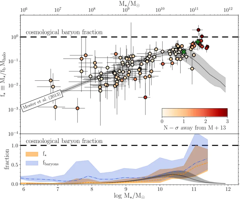
star formation efficiency, as a function of the stellar mass: we show this in Fig. 2. This plot highlights the two main find-ings of our work, the first being that f? appears to increase
A&A 626, A56 (2019)
10
610
710
810
910
1010
1110
1210
−410
−310
−210
−110
0f
?≡
M
?/f
bM
halo Moster et al. (2013)cosmological baryon fraction
0
1
2
3
N
− σ away from M + 13
10
610
710
810
910
1010
1110
12M
?/M
6
7
8
9
10
11
12
log M
?/M
0.0
0.5
1.0
fraction
cosmological baryon fraction
f
?f
baryonsFig. 2.Stellar fraction as a function of stellar mass for 110 galaxies in the SPARC sample. Top panel (in log-scale): individual measurements with their uncertainties. Bottom panel (in linear-scale): f?(orange dashed line) and fbaryons= f?+ 1.4 fHI+ fH2(blue dot-dashed line; see text for
details) in bins of log M?(shaded areas are the 1σ uncertainties). In both panels, the stellar-to-halo mass relation estimated byMoster et al.(2013) using abundance matching is shown as a black curve, with a shaded area representing its scatter. Points in the top panel are colour-coded by how many standard deviations away the galaxy is from theMoster et al.(2013) relation, i.e. | f?− f?,M+13|/(σ2f?+ σ
2
M+13)1/2, where σf?is the observed
uncertainty on f?, f?,M+13is the value predicted by the abundance matching model, and σM+13is the scatter of theMoster et al.(2013) relation. In both panels, galaxies that have converted all the available baryons in the halo into stars would lie on the long dashed line, whose thickness encompasses uncertainties on fb. As in Fig.1, also shown is the location of the Milky Way (cross) and the Andromeda galaxy (plus), as given by the modelling byPosti & Helmi(2019) andCorbelli et al.(2010), respectively.
monotonically with galaxy stellar mass with no indication of a peak in the range 10 ≤ log M?/M ≤ 11, where most abundance
matching models find a maximum star formation efficiency. For instance, a galaxy with M? = 2 × 10¹¹M has f? ' 0.04 in the Moster et al.(2013) model, while we find f?' 0.5. By comput-ing the difference between the measured f?and that expected in theMoster et al.(2013) model, normalised by the sum in quadra-ture of the measured uncertainty on f?and of the intrinsic scatter
of the model, we find the measurement for the high-mass sys-tems to be inconsistent at 2−3σ with the model (see the coloured points in Fig.2). This discrepancy is very robust and holds for all the tests we have run (see the f?−M?diagram in all these cases,
Fig.A.2):
– we fit the rotation curves assuming a cored (Burkert 1995) instead of a cuspy (NFW) profile. In general, this yields bet-ter fits for many low-mass systems, slightly higher stellar masses, and lower halo virial masses for all galaxies; – we used the fits recently obtained byGhari et al.(2019), who
usedEinasto(1965) halo profiles (and distances and mass-to-light ratios fromLi et al. 2018). In general, we typically find slightly lower halo virial masses, but broadly consistent with our estimates with NFW profiles;
– we fixed the mass-to-light ratio of the bulge and disc com-ponents to reasonable values suggested by stellar popula-tion synthesis models (Υdisc = 0.5, Υbulge = 0.7, see e.g. Meidt et al. 2014;Schombert & McGaugh 2014);
– we tried allowing bothΥdiscandΥbulgeto vary in our fits, with
the additional constraint ofΥdisc≤Υbulge. This had an effect
only on the 28 galaxies (out of 110) in our final sample that have non-negligible bulges. We find the resulting uncertain-ties onΥdiscto be significantly larger in this case, but never
dramatically so.
In all these cases the final result is that the f?−M?diagram is not
significantly different from that presented in Fig.2. Additionally, as shown by Katz et al. (2014, see their Figs. 20 and 23), the effect of adiabatic contraction of the dark matter halos due to the formation of stellar discs has a negligible impact on f? for galaxies in the interested mass regime.
The other main finding highlighted by Fig.2is even more surprising: we find that all spirals with M? & 1011M have a
stellar fraction very close to unity, in the range f? ≈ 0.3−1; a handful of them are consistent with f? = 1 within the
uncer-tainties. This implies that these galaxies were extremely efficient at turning gas into stars and that the amount of mass col-lapsed in stars is a considerable portion of the total amount of baryons expected to be associated with their halos. In fact, if we also include the contribution of atomic and molecular hydro-gen (the latter estimated through the MHI−MH2relation given by
Catinella et al. 2018), spirals with M?≥ 1011M are found to be
consistent with a cold baryon budget of fbaryons = f?+ 1.4 fHI+
fH2 ≈ 1 within the uncertainties (where the factor 1.4 accounts for helium, e.g.Lelli et al. 2016a), with a mean value of ∼0.6 and uncertainties of [−0.3,+0.5]. Moreover, considering that galax-ies are known to be surrounded by massive, hot coronae, which are detected in X-rays and with the Sunyaev–Zeldovich effect, and account for about 0.1−0.3 fbMhalo(typically estimated
statis-tically by stacking over many galaxies with a given stellar mass, e.g.Planck Collaboration Int. XI 2013;Bregman et al. 2018, and references therein), the total (cold+hot) baryon budget is easily compatible with unity at the high-mass end, with very little room for other baryonic components. In other words, we have found that the most massive, regularly rotating spirals in the nearby Universe have virtually no missing baryons.
4. Discussion
Our analysis provided us with a robust and unbiased estimate of the halo virial mass for a sample of 108 spiral galaxies in the nearby Universe using their high-quality Hi rotation curves. While we find good agreement with previous determinations of the stellar-to-halo mass relation for galaxies roughly up to the mass of the Milky Way (M? = 5 × 10¹⁰M ), we also find
sys-tematically lower halo masses (factor ∼10), corresponding to higher stellar-to-halo mass ratios, for the most massive spirals with respect to expectations from most up-to-date abundance matching models (e.g.Wechsler & Tinker 2018).
A possible explanation for this discrepancy is that while the high-mass end (M? & 1011M
) of the galaxy stellar mass
function is vastly dominated by passive early-type galaxies that occupy massive (Mhalo & 5 × 10¹²M ) dark matter halos, there
still exists a population of star-forming spirals that inhabit halos of lower masses. The presence of this second population – which is not well represented by current abundance matching mod-els – implies the existence of different evolutionary pathways for building galaxies of a given stellar mass. This suggests, for example, that a massive system that has evolved in isolation may have had the chance to sustain star formation unimpeded for its entire life, potentially converting most of its available baryons into stars. While this is certainly not the case for high-mass early-types galaxies, which tend to live in high-density
environments, it may well be the pathway taken by the high-mass population of spirals studied in this work.McGaugh et al.
(2010), by simply analysing the Tully–Fisher relation of a sim-ilar sample of spirals, also concluded that f?does not turn over at the highest masses.
A discrepancy between the expected halo mass for a typ-ical passive (red) 1011M
galaxy and an active (blue) galaxy
of the same stellar mass, was also noted by other authors using various probes, such as satellite kinematics (e.g. Conroy et al. 2007;More et al. 2011;Wojtak & Mamon 2013), galaxy–galaxy weak lensing (e.g. Mandelbaum et al. 2006,2016; Reyes et al. 2012), abundance matching (e.g.Rodríguez-Puebla et al. 2015), or combinations (e.g.Dutton et al. 2010). The works most sim-ilar to ours are those of K17 andLapi et al.(2018). We use the same galaxy sample as in K17 (SPARC) and we perform an anal-ysis that is similar to theirs, but with the crucial difference that we do not impose a prior on halo mass that follows an M?−Mhalo
relation from abundance matching, which slightly biases some of the high-mass galaxies towards higher halo masses4.Lapi et al.
(2018), on the other hand, have a much larger sample of spirals than ours, but they rely on stacked rotation curves for their mass decompositions, i.e. they stack individual curves of galaxies in bins of absolute magnitude, whereas we focus on individual, well-studied systems. Finally, we note that, amongst the detailed studies of individual systems, Corbelli et al. (2010) measured the dynamical mass of M31 by decomposing its Hi rotation curve, to find a surprisingly high f?' 0.6, andMartinsson et al.
(2013) decomposed the Hi rotation curves of a small sample of 30 spirals from the DiskMass Survey to find the highest star formation efficiencies f? & 0.3 for their three most
mas-sive galaxies (log M?/M & 10.9). While our results align with
these previous works, to our knowledge we are the first to focus specifically on the f?−M?relation and to highlight the fact that (i) the highest mass spirals are the most efficient galaxies at turn-ing gas into stars, (ii) f? increases monotonically with stellar mass for regularly rotating nearby discs, and (iii) virtually all high-mass discs have &30% of the total baryons within their halos in stars.
Our analysis establishes that the most efficient galaxies at forming stars are not L∗ galaxies, as previously thought (e.g.
Wechsler & Tinker 2018), but much more massive systems, some of the most massive spiral galaxies in the nearby Universe (M? & 1011M
). Not only does the galactic star-formation e
ffi-ciency peak at much higher masses than we knew before, but we also showed that several massive discs have efficiencies f?
of the order unity. This result alone is of key importance since it demonstrates that there is no universal physical mechanism that sets the maximum star formation efficiency to 20−30%.
Furthermore, the fact that some massive galaxies with high f?exist has fundamental implications for star formation
quench-ing. Since these galaxies live in halos with Mhalo ∼ 2−5 ×
1012M
, if mass is the main driver of quenching and if a
crit-ical mass for quenching exists (e.g. as expected in scenarios where virial shock heating of the circumgalactic medium is the key process, see Birnboim & Dekel 2003; Dekel & Birnboim 2008), then it follows that this critical mass cannot be lower than ∼5 × 10¹²M
, which is almost an order of magnitude higher than
previously thought (e.g.Dekel & Birnboim 2006). Interestingly, 4 Taking into account this difference in the priors used, our results are very well compatible with theirs: our conclusions sit in the middle between their case with uniform priors (their Fig. 3) and that in which they impose a prior following theMoster et al.(2013) M?−Mhalo rela-tion (their Fig. 5).
A&A 626, A56 (2019)
such a high threshold is instead expected in scenarios where the accretion of cool gas is hampered (“starvation”), for example by the high virial temperature of the circumgalactic gas in a galac-tic fountain cycle (e.g.Armillotta et al. 2016) or by the complex interplay of radiative cooling and feedback in the smooth gas accretion from cold filaments (e.g.van de Voort et al. 2011).
Even if we have measured high f? for some massive
spi-rals, the vast majority of galaxies living in Mhalo > 1012M
halos still have f? 1, which means that they managed to
efficiently quench their star formation. Our results imply that since mass cannot be the major player in quenching galax-ies, at least for Mhalo . 5 × 10¹²M , some other mechanism
must play a fundamental role in the transition from active to passive star formation. One of the main suspects is environ-ment, since gas removal happens more frequently and also gas accretion is more difficult in high-density environments (e.g.
Peng et al. 2010;van de Voort et al. 2017). Another is the pow-erful feedback from the active galactic nucleus (AGN), which can episodically suppress any gas condensation throughout the galaxy (e.g. Croton et al. 2006;Fabian 2012). Finally, another key process is the interaction with other galaxies, with passive galaxies being hosted in halos with an active merger history, which can result in bursty star formation histories and subse-quent suppressive stellar/AGN feedback (e.g.Cox et al. 2006a;
Gabor et al. 2010). This scenario also naturally accounts for the morphological transformation of disc galaxies, living in halos with quiet merger histories, to spheroids, which are the dominant galaxy population at the high-mass end, where mergers are also more frequent (e.g.Cox et al. 2006b). This scenario is, in prin-ciple, testable with current cosmological simulations and with a new abundance matching model that depends on secondary halo parameters, such as merger history or formation time, and it is able to predict not only stellar masses but also other galaxy prop-erties, such as morphology or colour.
Acknowledgements. We thank E. Corbelli, B. Famaey, A. Lapi, F. Lelli, A. Robertson, J. Sellwood, and F. van den Bosch for the useful discussions and A. Ghari for making the Einasto fits available to us. LP acknowledges finan-cial support from a VICI grant from the Netherlands Organisation for Scientific Research (NWO) and from the Centre National d’Etudes Spatiales (CNES).
References
Armillotta, L., Fraternali, F., & Marinacci, F. 2016,MNRAS, 462, 4157
Behroozi, P. S., Conroy, C., & Wechsler, R. H. 2010,ApJ, 717, 379
Birnboim, Y., & Dekel, A. 2003,MNRAS, 345, 349
Bregman, J. N. 2007,ARA&A, 45, 221
Bregman, J. N., Anderson, M. E., Miller, M. J., et al. 2018,ApJ, 862, 3
Burkert, A. 1995,ApJ, 447, L25
Cappellari, M., Scott, N., Alatalo, K., et al. 2013,MNRAS, 432, 1709
Catinella, B., Saintonge, A., Janowiecki, S., et al. 2018,MNRAS, 476, 875
Conroy, C., Prada, F., Newman, J. A., et al. 2007,ApJ, 654, 153
Corbelli, E., Lorenzoni, S., Walterbos, R., Braun, R., & Thilker, D. 2010,A&A, 511, A89
Cox, T. J., Jonsson, P., Primack, J. R., & Somerville, R. S. 2006a,MNRAS, 373, 1013
Cox, T. J., Dutta, S. N., Di Matteo, T., et al. 2006b,ApJ, 650, 791
Croton, D. J., Springel, V., White, S. D. M., et al. 2006,MNRAS, 365, 11
de Blok, W. J. G., McGaugh, S. S., Bosma, A., & Rubin, V. C. 2001,ApJ, 552, L23
Dekel, A., & Birnboim, Y. 2006,MNRAS, 368, 2
Dekel, A., & Birnboim, Y. 2008,MNRAS, 383, 119
Desmond, H., & Wechsler, R. H. 2015,MNRAS, 454, 322
Dutton, A. A., & Macciò, A. V. 2014,MNRAS, 441, 3359
Dutton, A. A., Conroy, C., van den Bosch, F. C., Prada, F., & More, S. 2010,
MNRAS, 407, 2
Einasto, J. 1965,Trudy Astrofizicheskogo Instituta Alma-Ata, 5, 87
Fabian, A. C. 2012,ARA&A, 50, 455
Foreman-Mackey, D., Hogg, D. W., Lang, D., & Goodman, J. 2013,PASP, 125, 306
Fukugita, M., Hogan, C. J., & Peebles, P. J. E. 1998,ApJ, 503, 518
Gabor, J. M., Davé, R., Finlator, K., & Oppenheimer, B. D. 2010,MNRAS, 407, 749
Ghari, A., Famaey, B., Laporte, C., & Haghi, H. 2019,A&A, 623, A123
Katz, H., McGaugh, S. S., Sellwood, J. A., & de Blok, W. J. G. 2014,MNRAS, 439, 1897
Katz, H., Lelli, F., McGaugh, S. S., et al. 2017,MNRAS, 466, 1648
Kelvin, L. S., Driver, S. P., Robotham, A. S. G., et al. 2014,MNRAS, 444, 1647
Kravtsov, A. V., Berlind, A. A., Wechsler, R. H., et al. 2004,ApJ, 609, 35
Lange, J. U., van den Bosch, F. C., Zentner, A. R., Wang, K., & Villarreal, A. S. 2018, MNRAS, submitted [arXiv:1811.03596]
Lapi, A., Salucci, P., & Danese, L. 2018,ApJ, 859, 2
Leauthaud, A., Tinker, J., Bundy, K., et al. 2012,ApJ, 744, 159
Lelli, F., McGaugh, S. S., & Schombert, J. M. 2016a,AJ, 152, 157
Lelli, F., McGaugh, S. S., & Schombert, J. M. 2016b,ApJ, 816, L14
Li, P., Lelli, F., McGaugh, S., & Schombert, J. 2018,A&A, 615, A3
Mandelbaum, R., Seljak, U., Kauffmann, G., Hirata, C. M., & Brinkmann, J. 2006,MNRAS, 368, 715
Mandelbaum, R., Wang, W., Zu, Y., et al. 2016,MNRAS, 457, 3200
Martinsson, T. P. K., Verheijen, M. A. W., Westfall, K. B., et al. 2013,A&A, 557, A131
McConnachie, A. W. 2012,AJ, 144, 4
McGaugh, S. S., & Schombert, J. M. 2014,AJ, 148, 77
McGaugh, S. S., Schombert, J. M., de Blok, W. J. G., & Zagursky, M. J. 2010,
ApJ, 708, L14
Meidt, S. E., Schinnerer, E., van de Ven, G., et al. 2014,ApJ, 788, 144
More, S., van den Bosch, F. C., Cacciato, M., et al. 2011,MNRAS, 410, 210
Moster, B. P., Naab, T., & White, S. D. M. 2013,MNRAS, 428, 3121
Navarro, J. F., Frenk, C. S., & White, S. D. M. 1996,ApJ, 462, 563
Papastergis, E., Cattaneo, A., Huang, S., Giovanelli, R., & Haynes, M. P. 2012,
ApJ, 759, 138
Peng, Y.-J., Lilly, S. J., Kovaˇc, K., et al. 2010,ApJ, 721, 193
Persic, M., & Salucci, P. 1992,MNRAS, 258, 14
Persic, M., Salucci, P., & Stel, F. 1996,MNRAS, 281, 27
Planck Collaboration VI. 2018, A&A, submitted [arXiv:1807.06209] Planck Collaboration Int. XI. 2013,A&A, 557, A52
Posti, L., & Helmi, A. 2019,A&A, 621, A56
Read, J. I., Iorio, G., Agertz, O., & Fraternali, F. 2017,MNRAS, 467, 2019
Reyes, R., Mandelbaum, R., Gunn, J. E., et al. 2012,MNRAS, 425, 2610
Rodríguez-Puebla, A., Avila-Reese, V., Yang, X., et al. 2015,ApJ, 799, 130
Salucci, P., & Burkert, A. 2000,ApJ, 537, L9
Schombert, J., & McGaugh, S. 2014,PASA, 31, e036
Starkman, N., Lelli, F., McGaugh, S., & Schombert, J. 2018,MNRAS, 480, 2292
Tumlinson, J., Peeples, M. S., & Werk, J. K. 2017,ARA&A, 55, 389
Vale, A., & Ostriker, J. P. 2004,MNRAS, 353, 189
van den Bosch, F. C., Norberg, P., Mo, H. J., & Yang, X. 2004,MNRAS, 352, 1302
van de Voort, F., Schaye, J., Booth, C. M., Haas, M. R., & Dalla Vecchia, C. 2011,MNRAS, 414, 2458
van de Voort, F., Bahé, Y. M., Bower, R. G., et al. 2017,MNRAS, 466, 3460
Wechsler, R. H., & Tinker, J. L. 2018,ARA&A, 56, 435
White, S. D. M., & Rees, M. J. 1978,MNRAS, 183, 341
Wojtak, R., & Mamon, G. A. 2013,MNRAS, 428, 2407
Yang, X., Mo, H. J., & van den Bosch, F. C. 2008,ApJ, 676, 248
Zheng, Z., Coil, A. L., & Zehavi, I. 2007,ApJ, 667, 760
Appendix A: Supplementary material
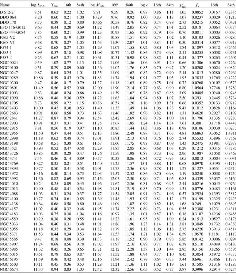
Table A.1. Results of the fits for individual galaxies.
Name log L[3.6] Υdisc 16th 84th log Mhalo 16th 84th log c 16th 84th χ2red f? 16th 84th
D 512-2 8.51 0.62 0.22 1.02 9.91 9.59 10.26 0.98 0.86 1.11 1.05 0.0852 0.0157 0.2845 DDO 064 8.20 0.60 0.21 1.00 10.29 9.76 10.92 1.00 0.83 1.17 1.07 0.0237 0.0029 0.1213 DDO 170 8.73 0.38 0.12 0.80 10.66 10.58 10.76 0.82 0.74 0.88 2.73 0.0215 0.0052 0.0431 ESO 116-G012 9.63 0.44 0.20 0.69 11.72 11.49 12.05 0.89 0.74 1.01 2.52 0.0181 0.0064 0.0374 ESO 444-G084 7.85 0.60 0.21 0.99 11.23 10.93 11.65 0.92 0.79 1.03 0.76 0.0011 0.0003 0.0030 F565-V2 8.75 0.58 0.19 1.00 11.14 10.88 11.51 0.89 0.73 1.02 1.10 0.0103 0.0026 0.0280 F568-V1 9.58 0.70 0.27 1.05 11.63 11.30 12.07 1.01 0.84 1.15 0.30 0.0314 0.0077 0.0919 F574-1 9.82 0.68 0.27 1.03 11.29 11.07 11.55 0.92 0.80 1.03 1.84 0.1097 0.0312 0.2466 F583-1 8.99 0.57 0.18 0.98 11.08 10.77 11.42 0.86 0.73 0.98 2.11 0.0255 0.0058 0.0731 F583-4 9.23 0.62 0.21 1.02 10.61 10.31 10.98 0.98 0.82 1.11 0.44 0.1377 0.0263 0.4602 NGC 0024 9.59 1.02 0.77 1.15 11.27 11.06 11.56 1.06 0.91 1.20 0.66 0.1306 0.0670 0.2269 NGC 0100 9.51 0.29 0.09 0.60 11.36 11.02 11.76 0.85 0.70 0.97 1.20 0.0208 0.0024 0.0820 NGC 0247 9.87 0.64 0.25 1.01 11.35 11.09 11.62 0.82 0.72 0.90 2.14 0.1013 0.0280 0.2969 NGC 0289 10.86 0.59 0.43 0.76 11.83 11.74 11.94 0.91 0.77 1.05 1.95 0.2833 0.1765 0.4227 NGC 0300 9.47 0.46 0.17 0.79 11.37 11.18 11.63 0.89 0.75 1.01 0.72 0.0268 0.0102 0.0573 NGC 0801 11.49 0.56 0.52 0.60 12.00 11.90 12.14 0.77 0.63 0.90 6.80 1.0564 0.7746 1.3789 NGC 1003 9.83 0.46 0.24 0.66 11.49 11.39 11.62 0.78 0.67 0.88 3.09 0.0485 0.0240 0.0746 NGC 1090 10.86 0.48 0.36 0.59 11.72 11.63 11.84 0.94 0.80 1.07 2.50 0.3931 0.2445 0.5734 NGC 1705 8.73 0.99 0.72 1.15 10.86 10.57 11.26 1.16 0.99 1.31 0.66 0.0352 0.0133 0.0712 NGC 2403 10.00 0.42 0.30 0.53 11.40 11.33 11.49 1.14 1.06 1.23 9.47 0.1012 0.0828 0.1164 NGC 2683 10.91 0.66 0.58 0.73 11.63 11.46 11.82 0.96 0.82 1.11 1.31 0.4620 0.2927 0.7192 NGC 2841 11.27 0.87 0.79 0.94 12.54 12.42 12.69 0.88 0.76 1.00 1.81 0.1796 0.1335 0.2283 NGC 2903 10.91 0.37 0.31 0.41 11.75 11.67 11.85 1.24 1.14 1.34 7.61 0.3001 0.1718 0.4448 NGC 2915 8.81 0.56 0.19 0.97 11.10 10.85 11.44 1.03 0.86 1.18 0.98 0.0106 0.0030 0.0270 NGC 2955 11.50 0.47 0.44 0.51 12.13 11.80 12.48 0.88 0.71 1.03 4.81 0.6863 0.3052 1.4911 NGC 2998 11.18 0.62 0.48 0.74 12.01 11.91 12.13 0.91 0.76 1.06 2.74 0.5532 0.3896 0.7568 NGC 3198 10.58 0.51 0.38 0.61 11.67 11.60 11.75 0.98 0.87 1.09 1.43 0.2475 0.1981 0.2979 NGC 3521 10.93 0.52 0.47 0.58 12.29 11.83 12.85 0.86 0.68 1.03 0.29 0.1212 0.0315 0.3787 NGC 3726 10.85 0.39 0.28 0.47 11.76 11.59 11.98 0.87 0.73 1.02 2.96 0.1987 0.1058 0.3469 NGC 3741 7.45 0.46 0.14 0.89 10.57 10.33 10.86 0.84 0.72 0.95 1.05 0.0013 0.0004 0.0031 NGC 3769 10.27 0.35 0.21 0.51 11.40 11.25 11.57 1.01 0.88 1.14 0.68 0.0970 0.0495 0.1719 NGC 3893 10.77 0.50 0.41 0.58 12.01 11.75 12.36 0.95 0.78 1.11 1.27 0.1227 0.0551 0.2310 NGC 3972 10.16 0.40 0.14 0.73 12.03 11.57 12.52 0.86 0.70 0.98 1.19 0.0240 0.0038 0.1250 NGC 3992 11.36 0.82 0.69 0.93 12.15 12.03 12.30 0.90 0.74 1.05 0.85 0.4339 0.3037 0.6160 NGC 4010 10.24 0.25 0.09 0.45 11.96 11.62 12.36 0.81 0.68 0.95 2.44 0.0216 0.0045 0.0764 NGC 4013 10.90 0.48 0.41 0.54 11.98 11.81 12.19 0.85 0.70 0.99 1.31 0.0776 0.0483 0.1161 NGC 4088 11.03 0.31 0.24 0.37 11.77 11.54 12.05 0.91 0.74 1.06 0.57 0.2924 0.1393 0.5817 NGC 4100 10.77 0.74 0.61 0.85 11.69 11.48 11.93 0.97 0.81 1.12 1.27 0.4199 0.2325 0.7423 NGC 4138 10.64 0.68 0.58 0.80 11.46 11.09 11.82 0.99 0.82 1.16 1.68 0.2491 0.1029 0.6693 NGC 4157 11.02 0.40 0.32 0.48 11.95 11.74 12.22 0.89 0.73 1.04 0.55 0.2388 0.1231 0.4311 NGC 4183 10.03 0.75 0.38 1.04 11.16 10.97 11.35 1.01 0.87 1.13 0.18 0.3102 0.1236 0.6488 NGC 4559 10.29 0.38 0.20 0.55 11.41 11.23 11.61 0.95 0.81 1.09 0.24 0.1513 0.0527 0.3176 NGC 5033 11.04 0.40 0.31 0.48 11.91 11.86 11.96 1.23 1.14 1.31 3.81 0.3049 0.1732 0.4383 NGC 5055 11.18 0.32 0.29 0.34 11.82 11.79 11.85 1.12 1.06 1.18 2.75 0.4220 0.3913 0.4514 NGC 5371 11.53 0.44 0.34 0.53 11.64 11.53 11.74 1.21 1.02 1.34 6.59 1.9570 1.1181 3.1110 NGC 5585 9.47 0.18 0.08 0.30 11.33 11.18 11.52 0.90 0.79 0.98 5.85 0.0142 0.0006 0.0294 NGC 5907 11.24 0.68 0.56 0.78 12.02 11.93 12.16 0.89 0.71 1.07 6.38 0.5110 0.4049 0.6183 NGC 5985 11.32 0.45 0.26 0.65 12.21 12.12 12.28 1.37 1.30 1.44 2.85 0.3156 0.1265 0.5595 NGC 6015 10.51 0.78 0.65 0.87 11.67 11.52 11.88 0.94 0.77 1.10 8.45 0.3054 0.1972 0.4377 NGC 6195 11.59 0.46 0.42 0.48 12.16 11.94 12.42 0.79 0.64 0.93 3.44 0.6961 0.3866 1.1779 NGC 6503 10.11 0.45 0.36 0.53 11.28 11.21 11.36 1.11 1.02 1.19 1.61 0.1585 0.1316 0.1883 NGC 6674 11.33 0.94 0.83 1.03 12.42 12.32 12.56 0.65 0.52 0.77 3.87 0.3996 0.2914 0.5274 Notes. The near-infrared luminosity L[3.6]is given in solar luminosities; the posteriors of the three model parameters, disc mass-to-light ratioΥdisc, halo mass Mhalo, and concentration c are represented with their 50th-16th-84th percentiles; χ2redis the reduced χ
2(Eq. (2)) for the best-fit model; the posterior on the derived parameter f?= M?/ fbMhalois represented with its 50th-16th-84th percentiles.
A&A 626, A56 (2019) Table A.1. continued.
Name log L[3.6] Υdisc 16th 84th log Mhalo 16th 84th log c 16th 84th χ2red f? 16th 84th NGC 6946 10.82 0.44 0.38 0.48 11.83 11.62 12.12 0.95 0.79 1.09 1.88 0.2336 0.1103 0.4250 NGC 7331 11.40 0.36 0.33 0.40 12.38 12.21 12.60 0.85 0.71 0.98 0.80 0.1527 0.0945 0.2232 NGC 7814 10.87 0.50 0.43 0.56 12.21 12.01 12.50 1.01 0.86 1.15 1.30 0.1245 0.0688 0.1869 UGC 00128 10.08 0.53 0.18 0.92 11.56 11.53 11.59 0.93 0.86 0.99 3.19 0.1058 0.0370 0.1797 UGC 00191 9.30 0.83 0.51 1.08 10.96 10.87 11.10 0.93 0.82 1.02 3.68 0.0947 0.0586 0.1368 UGC 00731 8.51 0.59 0.19 1.01 10.77 10.64 10.91 0.99 0.91 1.08 0.36 0.0176 0.0051 0.0338 UGC 02259 9.24 0.86 0.46 1.11 10.78 10.69 10.89 1.23 1.15 1.31 1.37 0.1220 0.0610 0.1851 UGC 02487 11.69 0.98 0.85 1.08 12.58 12.52 12.67 0.94 0.81 1.06 5.28 0.3968 0.3302 0.4704 UGC 02885 11.61 0.63 0.55 0.72 12.62 12.48 12.79 0.75 0.62 0.88 1.47 0.3448 0.2284 0.5073 UGC 02916 11.09 0.34 0.31 0.36 12.10 11.93 12.31 1.05 0.95 1.15 10.88 0.2354 0.1404 0.3645 UGC 02953 11.41 0.56 0.51 0.60 12.29 12.22 12.36 1.11 1.02 1.20 6.78 0.4796 0.3421 0.6312 UGC 03205 11.06 0.72 0.64 0.79 12.12 11.95 12.33 0.85 0.70 1.01 3.51 0.4040 0.2531 0.5862 UGC 03546 11.01 0.41 0.34 0.46 11.92 11.80 12.06 1.07 0.96 1.18 1.52 0.2236 0.1352 0.3344 UGC 03580 10.12 0.18 0.13 0.22 11.52 11.42 11.64 0.95 0.87 1.04 3.52 0.0459 0.0121 0.0823 UGC 04278 9.12 0.36 0.10 0.76 11.41 11.00 11.89 0.80 0.65 0.94 2.19 0.0095 0.0011 0.0430 UGC 04483 7.11 0.52 0.17 0.93 9.30 8.97 9.74 1.11 0.95 1.26 0.74 0.0160 0.0038 0.0485 UGC 04499 9.19 0.34 0.11 0.69 10.89 10.70 11.12 0.93 0.81 1.04 0.95 0.0322 0.0070 0.0839 UGC 05005 9.61 0.36 0.10 0.78 11.10 10.84 11.36 0.85 0.71 0.97 1.11 0.0718 0.0151 0.2207 UGC 05253 11.23 0.46 0.43 0.48 12.16 12.08 12.27 1.05 0.98 1.12 3.22 0.3759 0.2567 0.5165 UGC 05414 9.05 0.20 0.06 0.46 11.17 10.82 11.57 0.77 0.64 0.89 1.68 0.0061 0.0002 0.0256 UGC 05716 8.77 0.44 0.15 0.83 10.81 10.75 10.89 0.98 0.91 1.03 1.76 0.0186 0.0062 0.0312 UGC 05721 8.73 0.93 0.60 1.12 10.91 10.68 11.23 1.17 1.01 1.30 1.90 0.0317 0.0142 0.0596 UGC 05829 8.75 0.59 0.18 1.01 10.47 10.16 10.83 0.95 0.80 1.09 0.84 0.0539 0.0106 0.1593 UGC 05918 8.37 0.63 0.21 1.02 10.07 9.81 10.43 1.04 0.89 1.17 0.35 0.0580 0.0124 0.1611 UGC 06399 9.36 0.61 0.22 0.99 11.27 10.95 11.67 0.89 0.75 1.02 0.97 0.0362 0.0077 0.1135 UGC 06446 8.99 0.75 0.32 1.08 10.96 10.75 11.23 1.06 0.92 1.18 0.22 0.0385 0.0133 0.0808 UGC 06614 11.09 0.27 0.17 0.36 12.20 12.03 12.41 0.83 0.68 0.96 0.44 0.0828 0.0428 0.1474 UGC 06667 9.15 0.63 0.21 1.03 11.41 11.18 11.72 0.88 0.76 0.98 1.57 0.0113 0.0029 0.0275 UGC 06786 10.87 0.57 0.49 0.65 12.22 12.10 12.37 1.05 0.94 1.16 1.47 0.1669 0.1166 0.2240 UGC 06787 10.99 0.43 0.38 0.47 12.17 12.10 12.24 1.19 1.12 1.26 27.20 0.2041 0.1410 0.2737 UGC 06917 9.83 0.46 0.18 0.78 11.46 11.23 11.77 0.93 0.79 1.05 0.75 0.0438 0.0137 0.1163 UGC 06923 9.46 0.30 0.11 0.59 11.20 10.83 11.68 0.94 0.78 1.08 0.85 0.0194 0.0035 0.0809 UGC 06930 9.95 0.68 0.28 1.02 11.15 10.93 11.38 0.99 0.86 1.12 0.33 0.2057 0.0617 0.4919 UGC 06973 10.73 0.18 0.16 0.20 12.83 12.24 13.53 0.86 0.65 1.06 1.11 0.0032 0.0006 0.0126 UGC 06983 9.72 0.76 0.38 1.06 11.31 11.11 11.57 1.00 0.85 1.13 0.70 0.0767 0.0301 0.1557 UGC 07089 9.55 0.44 0.13 1.05 10.68 9.71 11.15 0.91 0.75 1.13 1.01 0.1587 0.0203 3.9876 UGC 07125 9.43 0.28 0.09 0.57 10.46 10.33 10.60 0.91 0.81 1.01 1.08 0.1392 0.0239 0.3678 UGC 07151 9.36 0.84 0.58 1.06 10.77 10.45 11.14 0.95 0.80 1.07 2.64 0.1613 0.0586 0.4149 UGC 07399 9.06 0.84 0.45 1.10 11.39 11.17 11.70 1.13 1.01 1.23 1.74 0.0163 0.0066 0.0315 UGC 07524 9.39 0.50 0.17 0.94 11.00 10.77 11.27 0.87 0.75 0.97 0.94 0.0657 0.0155 0.1930 UGC 07559 8.04 0.53 0.15 1.02 9.31 8.70 9.76 1.08 0.92 1.27 1.29 0.1263 0.0185 1.0510 UGC 07603 8.58 0.53 0.20 0.88 11.01 10.70 11.44 0.97 0.82 1.11 1.62 0.0084 0.0021 0.0224 UGC 07690 8.93 0.89 0.66 1.08 10.18 9.87 10.53 1.09 0.94 1.25 0.48 0.1986 0.0754 0.4751 UGC 07866 8.09 0.66 0.22 1.06 9.31 8.78 9.80 1.14 0.97 1.30 0.23 0.1754 0.0266 0.9472 UGC 08286 9.10 0.94 0.61 1.13 10.90 10.78 11.05 1.11 1.02 1.20 2.13 0.0801 0.0490 0.1160 UGC 08490 9.01 0.92 0.58 1.12 10.79 10.64 10.99 1.15 1.01 1.27 0.29 0.0746 0.0425 0.1147 UGC 08550 8.46 0.79 0.42 1.07 10.51 10.33 10.74 1.05 0.93 1.16 0.66 0.0314 0.0154 0.0546 UGC 08699 10.70 0.56 0.51 0.60 11.95 11.75 12.21 0.99 0.85 1.11 1.13 0.1982 0.1076 0.3284 UGC 09037 10.84 0.11 0.04 0.20 11.91 11.74 12.13 0.87 0.74 0.98 1.03 0.0381 0.0101 0.0852 UGC 09133 11.45 0.47 0.44 0.50 12.22 12.18 12.25 0.99 0.92 1.05 8.84 0.5423 0.4231 0.6673 UGC 10310 9.24 0.73 0.30 1.06 10.67 10.42 10.96 1.02 0.88 1.14 0.49 0.1258 0.0341 0.3281 UGC 11820 8.99 0.52 0.17 0.90 11.15 11.04 11.28 0.74 0.65 0.81 2.20 0.0221 0.0079 0.0377 UGC 11914 11.18 0.64 0.61 0.67 13.04 12.44 13.67 0.75 0.58 0.94 2.55 0.0492 0.0110 0.2009 UGC 12506 11.14 0.97 0.66 1.14 12.14 11.96 12.33 0.99 0.84 1.13 0.67 0.5698 0.2753 0.9742 UGC 12632 9.11 0.66 0.23 1.04 10.73 10.56 10.92 0.98 0.87 1.09 0.41 0.0878 0.0252 0.1817 UGC 12732 9.22 0.54 0.18 0.95 11.11 10.96 11.30 0.92 0.80 1.02 0.29 0.0361 0.0109 0.0741 UGCA 281 8.29 0.66 0.28 1.01 9.86 9.36 10.46 1.04 0.88 1.18 0.89 0.0382 0.0054 0.1712 UGCA 444 7.08 0.61 0.21 1.02 9.62 9.19 10.14 1.08 0.91 1.25 0.55 0.0088 0.0018 0.0316 A56, page 8 of9
log Mhalo= 12.15+0.15−0.12 NGC3992 χ2 red= 1 log M?= 11.01+0.07−0.09 f?= 0.434+0.182−0.130 0.6 0.8 1.0 1.2 log c log c = 0.90+0.15−0.16 12.0 12.2 12.4 12.6 log Mhalo 0.45 0.60 0.75 0.90 1.05 Υ?,D 0.6 0.8 1.0 1.2 log c 0.45 0.60 0.75 0.90 1.05Υ?,D Υ?,D= 0.82+0.11−0.13 10 15 20 25 30 35 40 45
Radius/kpc
0 50 100 150 200 250V
elo
cit
y
/km
s
− 1V? Vgas VDM model Vrot
Fig. A.1.Example of rotation curve decomposition for NGC 3992. Left panel: observed rotation curve (black points) with our best model (red solid curve), decomposed into the contributions from stars (gold dashed curve), gas (blue dotted curve), and dark matter (purple dot-dashed curve). Right panel: posterior distributions of the three parameters of the model: halo mass, halo concentration, and mass-to-light ratio of the stellar disc. Similar plots for all the other galaxies in our sample can be found online athttp://astro.u-strasbg.fr/~posti/PFM19_fiducial_fits/.
107 109 1011 M?/M 10−5 10−4 10−3 10−2 10−1 100 101 f? ≡ M? /fb Mhalo NFW halo 0 1 2 3 N − σ aw ay from M + 13 107 109 1011 M?/M 10−5 10−4 10−3 10−2 10−1 100 101 f? ≡ M? /fb MBurk ert Burkert halo 0 1 2 3 N − σ aw ay from M + 13 107 109 1011 M?/M 10−5 10−4 10−3 10−2 10−1 100 101 f? ≡ M? /fb MEinasto Einasto halo 0 1 2 3 N − σ aw ay from M + 13 107 109 1011 M?/M 10−5 10−4 10−3 10−2 10−1 100 101 f? ≡ M? /fb Mhalo
Fixed (Υdisc, Υbulge) = (0.5, 0.7)
0 1 2 3 N − σ aw ay from M + 13 107 109 1011 M?/M 10−5 10−4 10−3 10−2 10−1 100 101 f? ≡ M? /fb Mhalo
Fitted (Υdisc, Υbulge)with Υdisc≤ Υbulge
0 1 2 3 N − σ aw ay from M + 13
Fig. A.2.Resulting f?−M?relation when varying the assumptions on the fit of the galaxy rotation curves. In the top row the dark matter halo model was varied: NFW (left), Burkert (centre), or Einasto (right). In the first two cases, the rotation curves were fit with a uniform prior onΥdisc, assumingΥbulge = 1.4Υdisc and with a prior on the concentration-mass relation for the NFW profile (fromDutton & Macciò 2014) and one on the core radius-core mass relation for the Burkert profile (fromSalucci & Burkert 2000). Instead, the fits in the Einasto case were obtained by
Ghari et al.(2019), who used the mass-to-light ratios derived byLi et al.(2018). In the bottom row, an NFW halo was used, but the assumptions on the mass-to-light ratios were varied: either fixed (left) or both left free to vary with the conditionΥdisc≤Υbulge(right). In all panels the colouring of the points, the dashed horizontal line, and the abundance matching predictions (dashed curve with grey band) are as in Fig.2.