HAL Id: hal-00329377
https://hal.archives-ouvertes.fr/hal-00329377
Submitted on 30 Mar 2005
HAL is a multi-disciplinary open access
archive for the deposit and dissemination of
sci-entific research documents, whether they are
pub-lished or not. The documents may come from
teaching and research institutions in France or
abroad, or from public or private research centers.
L’archive ouverte pluridisciplinaire HAL, est
destinée au dépôt et à la diffusion de documents
scientifiques de niveau recherche, publiés ou non,
émanant des établissements d’enseignement et de
recherche français ou étrangers, des laboratoires
publics ou privés.
boundaries and DMSP particle precipitation boundaries
in the morning sector ionosphere
G. Chisham, M. P. Freeman, T. Sotirelis, R. A. Greenwald, M. Lester, J.-P.
Villain
To cite this version:
G. Chisham, M. P. Freeman, T. Sotirelis, R. A. Greenwald, M. Lester, et al.. A statistical comparison
of SuperDARN spectral width boundaries and DMSP particle precipitation boundaries in the morning
sector ionosphere. Annales Geophysicae, European Geosciences Union, 2005, 23 (3), pp.733-743.
�hal-00329377�
SRef-ID: 1432-0576/ag/2005-23-733 © European Geosciences Union 2005
Annales
Geophysicae
A statistical comparison of SuperDARN spectral width boundaries
and DMSP particle precipitation boundaries in the morning sector
ionosphere
G. Chisham1, M. P. Freeman1, T. Sotirelis2, R. A. Greenwald2, M. Lester3, and J.-P. Villain4
1British Antarctic Survey, Natural Environment Research Council, High Cross, Madingley Road, Cambridge, CB3 0ET, UK 2Applied Physics Laboratory, Johns Hopkins University, 11100 Johns Hopkins Road, Laurel, MD 20723, USA
3Radio and Space Plasma Physics Group, University of Leicester, Leicester, LE1 7RH, UK 4LPCE/CNRS, 3A Avenue de la Recherche Scientifique, 45071 Orleans Cedex 2, France
Received: 2 November 2004 – Revised: 6 January 2005 – Accepted: 10 January 2005 – Published: 30 March 2005
Abstract. Determining reliable proxies for the ionospheric
signature of the open-closed field line boundary (OCB) is crucial for making accurate ionospheric measurements of many magnetospheric processes (e.g. magnetic reconnec-tion). This study compares the latitudes of Spectral Width Boundaries (SWBs), identified in the morning sector iono-sphere using the Super Dual Auroral Radar Network (Su-perDARN), with Particle Precipitation Boundaries (PPBs) determined using the low-altitude Defense Meteorological Satellite Program (DMSP) spacecraft, in order to determine whether the SWB represents a good proxy for the iono-spheric projection of the OCB. The latitudes of SWBs and PPBs were identified using automated algorithms applied to 5 years (1997–2001) of data measured in the 00:00– 12:00 Magnetic Local Time (MLT) range. A latitudinal difference was measured between each PPB and the near-est SWB within a ±10 min Universal Time (UT) window and within a ±1 h MLT window. The results show that the SWB represents a good proxy for the OCB close to midnight (∼00:00–02:00 MLT) and noon (∼08:00–12:00 MLT), but is located some distance (∼2◦–4◦) equatorward of the OCB across much of the morning sector ionosphere (∼02:00– 08:00 MLT). On the basis of this and other studies we de-duce that the SWB is correlated with the poleward boundary of auroral emissions in the Lyman-Birge-Hopfield “Long” (LBHL) UV emission range and hence, that spectral width is inversely correlated with the energy flux of precipitating electrons. We further conclude that the combination of two factors may explain the spatial distribution of spectral width values in the polar ionospheres. The small-scale structure of the convection electric field leads to an enhancement in spec-tral width in regions close to the OCB, whereas increases in ionospheric conductivity (relating to the level of incident electron energy flux) lead to a reduction in spectral width in regions just equatorward of the OCB.
Correspondence to: G. Chisham
(g.chisham@bas.ac.uk)
Keywords. Ionosphere (Particle precipitation; Instruments
and techniques) – Magnetospheric physics (Magnetopause, cusp and boundary layers)
1 Introduction
The boundary, or separatrix, between closed geomagnetic field lines with both foot points on the earth and open ge-omagnetic field lines with one end connected to the Inter-planetary Magnetic Field (IMF) is a key diagnostic for the magnetospheric system. This boundary is typically termed the Open-Closed field line Boundary (OCB), although its ionospheric projection is also known as the polar cap bound-ary. By identifying and tracking the OCB (in the ionosphere), the addition and removal of open magnetic flux can be mea-sured, and hence, the net global reconnection rate can be de-termined (Siscoe and Huang, 1985; Cowley and Lockwood, 1992; Milan et al., 2003, 2004). In combination with E×B velocity measurements at the boundary, the temporal and spatial structure of the magnetic reconnection rate can be de-termined (Baker et al., 1997; Pinnock et al., 2003)
There are a wide range of proxies which are used to iden-tify the OCB, including particle precipitation signatures mea-sured by low-altitude spacecraft (Newell et al., 1991; Newell and Meng, 1992; Newell et al., 1996a), optical signatures of precipitation measured by all-sky cameras, spacecraft im-agers, and meridian-scanning photometers (Blanchard et al., 1995, 1997; Sandholt et al., 1998; Brittnacher et al., 1999), E-region electron density signatures measured by incoherent scatter radar (de la Beaujardi`ere et al., 1994; Blanchard et al., 1996, 2001), the equatorward edge of HF radar backscat-ter (Milan et al., 1999; Milan and Lesbackscat-ter, 2001), and the Doppler Spectral Width Boundary (SWB) measured by the Super Dual Auroral Radar Network (SuperDARN) (Baker et al., 1995, 1997; Chisham et al., 2001, 2002). Particle measurements made by low-altitude spacecraft (such as the
Defense Meteorological Satellite Program (DMSP) space-craft) provide the most direct and precise determination of boundaries between different magnetospheric plasma regions (including the OCB) and hence provide the benchmark for other observational techniques. However, their usage is re-stricted as they only make snapshot observations of the Par-ticle Precipitation Boundaries (PPBs) in each polar region every ∼100 min orbit. Consequently, it is desirable to com-pare the open-closed PPBs with estimates of the OCB made by other instruments that have greater spatial coverage and higher temporal resolution. Studies to date have included comparisons with boundaries measured by ground-based im-agers (Blanchard et al., 1995, 1997) and UltraViolet Imim-agers (UVI) on spacecraft (Kauristie et al., 1999; Baker et al., 2000). The most comprehensive investigation of this type is that of Carbary et al. (2003). They compared ∼23 000 DMSP observations of the OCB with the poleward boundary of UVI auroral emissions measured by the Polar spacecraft. They showed that, statistically, the boundaries matched well (the median of the boundary differences being within 1◦ of zero difference) except in the early morning sector (∼00:00– 09:00 MLT) where the DMSP OCB was located ∼2◦–4◦ poleward of the UVI poleward boundary. However, some of this conclusion was based on an extrapolation of results as there were no DMSP data available in the 22:00–05:00 MLT sector.
Comparisons have also been made between PPBs and SWBs measured by the SuperDARN radars. The character-istics of Doppler spectra measured by the SuperDARN HF radars (Greenwald et al., 1995) have been shown to vary be-tween the ionospheric footprints of different magnetospheric regions (Andr´e et al., 2002). The Doppler spectral width is a measure of the spatial and temporal structure in the ionospheric electric field on scales comparable to, or less than, the radar integration period (∼1–10 s), and the spatial area of the radar observation cell (∼100 km square). This structure is typically a complex convolution of a number of factors (Andr´e et al., 2000b). The SWB is a latitudinal transition between radar backscatter with high and variable Doppler spectral width values, typically observed at high latitudes, and that with low Doppler spectral width values, typically observed at low latitudes (Freeman and Chisham, 2004). A SWB is readily observed at all magnetic local times, during all geomagnetic conditions (Chisham and Free-man, 2004). This transition typically occurs over a few de-grees of latitude, although the transition can be much sharper at times (Chisham and Freeman, 2004). Statistical compar-isons between PPBs and SWBs have shown the SWB to be a good proxy for the OCB in the cusp region ionosphere (Baker et al., 1995) and in the pre-midnight sector ionosphere (Chisham et al., 2004).
Away from the cusp and the pmidnight sector the re-lationship between the SWB and the different PPBs is un-clear. Chisham and Freeman (2004) suggested that the SWB in the morning sector ionosphere was most likely co-located with the OCB as the probability distribution of the latitude of preferred SWB locations formed a continuous ring from the
cusp, through the morning sector, to the pre-midnight sector. However, Woodfield et al. (2002) presented an event from the post-midnight sector where the SWB was located some distance equatorward of the poleward boundary of a region of 630 nm auroral emission, which has itself been shown to be a good proxy for the OCB in this sector (Blanchard et al., 1995). Similarly, in another case study, Wild et al. (2004) concluded that the SWB was not a good proxy for the OCB in the dawn sector. They compared PPBs from both low-altitude and high-altitude spacecraft with UVI data from the Imager for Magnetopause-to-Aurora Global Exploration (IMAGE) spacecraft, and with SuperDARN spectral width measurements. Measurements from around ∼04:00 MLT showed that the SWB was located close to, or just poleward of, the region of brightest auroral luminosity, a few degrees equatorward of the OCB determined from the spacecraft par-ticle precipitation measurements.
The aim of the present paper is to analyse statistically how the SWB relates to the OCB across the whole of the morn-ing sector ionosphere. To this end, we compare the latitudes of SWBs measured in the morning sector ionosphere in 5 years of data from 4 Northern Hemisphere, and 2 Southern Hemisphere, SuperDARN radars with the latitudes of PPBs observed by DMSP low-altitude spacecraft at similar UT and MLT. The existence of thousands of boundary comparisons allows us to make confident statements about the relationship of the SWB to the OCB, across the whole of the morning sec-tor ionosphere.
2 Analysis techniques
To make an accurate statistical comparison between Super-DARN SWBs and DMSP PPBs it is crucial that we have re-liable, objective techniques which can automatically identify these boundaries on a routine basis. Below, we detail the most reliable boundary determination techniques presently available and also the method of data comparison.
2.1 The spectral width boundary
We employ the “C-F threshold technique” (Chisham and Freeman, 2003, 2004) to identify the SWB. Threshold tech-niques have been employed to objectively identify the SWB in cusp-region SuperDARN backscatter for some years now (Baker et al., 1997; Chisham et al., 2001). These tech-niques involve choosing a spectral width threshold value above which the spectral width values are more likely to orig-inate from the distribution of spectral width values typically found in the cusp, and developing an algorithm that searches poleward along a radar beam until this threshold is exceeded. Chisham and Freeman (2003) showed that this technique can be inaccurate in its basic form as the probability distributions of the spectral width values poleward and equatorward of the SWB are typically broad and have considerable overlap (see also Freeman and Chisham, 2004). Chisham and Freeman (2003) showed that the inclusion of additional rules in the
threshold algorithm, such as spatially and temporally median filtering the spectral width data, increased the accuracy of the estimation of the SWB location. This led to the devel-opment of the C−F threshold technique, described in detail in Chisham and Freeman (2004), who also showed that the technique objectively identified SWBs at all MLTs. How-ever, SWBs rarely approximate infinitely sharp latitudinal transitions in spectral width, and hence, an analysis which uses multiple spectral width thresholds is often needed to determine the full structure and sharpness of the boundary (Chisham and Freeman, 2004).
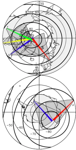
In this study we have applied the C−F threshold technique to 5 years of spectral width data (1997–2001 inclusive) from the meridional beams of SuperDARN radars from both hemi-spheres. We expect that meridional beams are most accu-rate for identifying the SWB because they are parallel to the spectral width gradient, assuming the alignment of the OCB (and hence the postulated spectral width proxy) is along an approximately constant geomagnetic latitude. In Fig. 1 we present the fields of view of the 6 SuperDARN radars em-ployed in this study – CUTLASS Finland (F), Goose Bay (G), Kapuskasing (K), Saskatoon (T), Halley (H), and Ker-guelen (P). The coloured beams highlight the meridional beams used.
The boundary databases for each radar were compiled in the following way:
1. We only used data from SuperDARN common mode operation intervals. This ensured that the radars were running exactly the same operational programs for all of the intervals in the database and that the processing of the raw data was consistent.
2. The spectral width values were extracted from the raw SuperDARN data using the same version of the Super-DARN data processing software (fitACF v.1.09) and us-ing a Lorentzian ACF fit.
3. Data flagged as ground backscatter during the raw data processing were removed; ground backscatter is typ-ically characterised by low Doppler velocity and low Doppler spectral width (Chisham and Pinnock, 2002). 4. Potential E-region backscatter at low ranges (< range
gate 10) was removed.
5. Backscatter with a signal power of less than 3 dB was removed.
6. The C-F threshold technique was applied blindly to the complete 5-year data sets for each radar using eight dif-ferent spectral width thresholds (ranging from 100 to 275 m/s). Most of the results presented in this paper are for a 200 m/s threshold, as in Chisham et al. (2004), al-though the differences which occur when using different thresholds will be discussed.
Fig. 1. Northern and Southern Hemisphere polar maps (geographic
coordinates) showing the fields of view of the SuperDARN radars employed in this study. The Northern Hemisphere radars used are CUTLASS Finland (F), Goose Bay (G), Kapuskasing (K), and Saskatoon (T). The Southern Hemisphere radars used are Halley (H) and Kerguelen (P). The bold black lines represent contours of constant altitude-adjusted corrected geomagnetic (AACGM) lati-tude (latilati-tudes as shown). The coloured beams represent the merid-ional beams for each radar as used in this study.
2.2 DMSP particle precipitation boundaries
In this study we make use of PPBs from 5 DMSP space-craft (F11–15) identified in particle measurements from the same 5-year interval (1997–2001). The nightside (00:00– 06:00 MLT) PPBs that we use are among those defined by Newell et al. (1996a,b) and are determined using the method outlined in Sotirelis and Newell (2000). This method per-forms post-processing checks which discard most failures of the boundary determination algorithm and remove ambigu-ous boundaries from the data set.
We use determinations of the following PPBs:
1. b1e, which is a proxy for the “zero-energy electron” convection boundary.
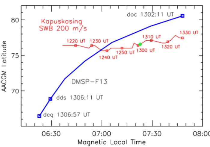
Fig. 2. An example boundary correlation from 1 April 2000. The
blue line represents the path of DMSP-F13 with PPBs marked as blue squares (boundary type and UT of observation shown). The red line represents the path of the 200 m/s threshold SWB for Ka-puskasing beam 11 (UTs of observations shown). The position of the SWB at the time of the OCB observation is indicated by the green diamond on the red line.
3. b4s, the unstructured/structured precipitation boundary, which is a proxy for the Central Plasma Sheet (CPS)-Boundary Plasma Sheet (BPS) boundary.
4. b6, which marks the poleward edge of the sub-visual drizzle region and which is a proxy for the OCB. This boundary occurs poleward of the main auroral oval and is characterized by either a drop in particle fluxes to be-low detectable levels or by the first encounter of a polar rain signature which signifies a transition to open field lines.
The dayside (06:00–12:00 MLT) PPBs that we use are based on the automated dayside region identification algo-rithms outlined by Newell et al. (1991) and are again deter-mined using the method of Sotirelis and Newell (2000).
We use determinations of the following PPBs:
1. deq, the equatorward boundary of diffuse precipitation, analogous to b1e on the nightside.
2. dds, the diffuse/structured precipitation boundary, anal-ogous to b4s on the nightside. This is located where there is an unambiguous transition from CPS precipita-tion to BPS precipitaprecipita-tion and/or low-latitude boundary layer (LLBL) precipitation.
3. doc, the open-closed field line boundary, analogous to b6 on the nightside. This is located where there is an un-ambiguous transition between open and closed field line precipitation regions. CPS, BPS, and LLBL are taken to be closed, and cusp, mantle, open LLBL, polar rain, and void are considered to be open.
If any of these transitions are not clear, because of ambi-guities in the region locations, then the transition is not added to the data set.
2.3 Data Comparison
The data comparison technique is the same as that used in Chisham et al. (2004). Taking the SWBs for each radar in turn, each PPB was matched with the closest SWB obtained within ±10 min UT of the PPB observation. The SWB obser-vation must also have been within ±1 h of MLT of the PPB observation to produce a matched boundary pair. Using this technique, a single PPB may be matched with more than one SWB, if the two SWBs originate from different radars. Fig-ure 2 presents an example of a boundary match. The blue line represents the path of DMSP-F13 between 13:02:11 UT and 13:06:57 UT on 1 April 2000, in AACGM latitude and MLT space. The labelled blue squares on the satellite path indicate the locations of the doc, dds, and deq boundaries measured during this overpass of the auroral oval. The red line repre-sents the path of the SWB (using a spectral width threshold of 200 m/s) measured at 2-min resolution by Kapuskasing beam 11. The red squares are UT markers, each separated by 10 min. The green diamond on the red line marks the SWB estimation closest in time to the doc boundary deter-mination (at 13:02 UT). These two boundary deterdeter-minations are less than 1 h of MLT apart (25 min) and so they comprise a matched pair. For this matched pair, the latitudinal differ-ence was determined to be 4.0◦. For each such matched pair, the difference between the two boundary latitudes was deter-mined.
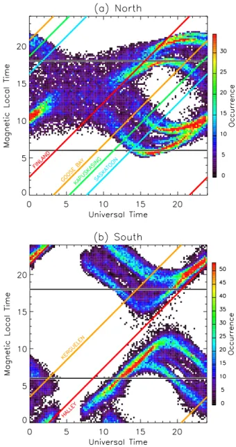
Ideally, it would have been preferable in the first instance to perform this study across the whole of the morning sec-tor ionosphere using SWBs from a single radar only, as was done in the pre-midnight sector by Chisham et al. (2004). This method would eliminate all other variables (such as dif-ferences resulting from geographic location and HF radio propagation conditions), that might have secondary effects on the spectral width. However, this is not possible because of the phasing of the DMSP spacecraft orbits. To illustrate this problem we present, in Fig. 3, a comparison of the UT-MLT coverage of the OCB proxies (b6 and doc) measured by the DMSP spacecraft with that of the meridional beams of the SuperDARN radars used in the study. Figure 3a presents the picture in the Northern Hemisphere and Fig. 3b presents the picture in the Southern Hemisphere. The coverage of the Su-perDARN meridional beams is shown by the bold diagonal coloured lines, one for each radar. Meridional beams have an almost constant UT-MLT offset along the beam (hence the narrow straight lines in UT-MLT space). The coverage of the DMSP PPBs is shown by the coloured shading which in-dicates the number of boundaries identified in each UT-MLT sector (UT-MLT sectors were chosen to be 0.2 by 0.2 h in size). The black horizontal lines (at 06:00 and 18:00 MLT) mark the transitions from nightside to dayside PPB identi-fication definitions. It is clear that the DMSP coverage of UT-MLT space is uneven, and very different in the two hemi-spheres. The overlap of DMSP PPB observations and radar coverage (even allowing for the 1-h MLT window when com-paring data sets) is very patchy, and no radar overlaps for more than ∼12 h of MLT. In the Northern Hemisphere, there
are almost no DMSP OCB observations between 00:00 and 06:00 MLT. Similarly, in the Southern Hemisphere, there are almost no DMSP OCB observations which overlap with the radar observations between 06:00 and 12:00 MLT. Hence, Fig. 3 illustrates the necessity of using comparisons with more than one SuperDARN radar to cover the whole morning sector ionosphere.
3 Results
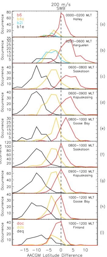
In Fig. 4 we show the occurrence distributions of the lati-tudinal differences between the different PPB types and the 200 m/s threshold SWB for a number of radars in different MLT ranges between 00:00 and 12:00 MLT. As we are using the results of comparisons with SWBs from more than one radar we choose initially to present results from each radar separately. The results are presented in the same format as Fig. 2 from Chisham et al. (2004), i.e. a stackplot of lati-tudinal difference distributions separated into different MLT ranges, and in this case, separated by radar. The distributions have a latitudinal resolution of 2◦except the Halley data in panel a, where the resolution is 1◦. The distributions are pre-sented relative to the SWB location (dashed vertical line at zero latitude difference). For the results from the nightside ionosphere (panels a and b in Fig. 4), the comparison is made for the b1e, b2i, b4s, and b6 boundaries. For the results from the dayside ionosphere (panels c to i in Fig. 4), the compar-ison is made for the deq, dds, and doc boundaries. Due to the method of presentation there are different panels which represent the same MLT range, but contain results from dif-ferent radars (e.g. panels e and f, which contain results from 08:00–10:00 MLT but from Goose Bay and Saskatoon, re-spectively).
A clear pattern is evident in the results presented in Fig. 4. The deq (black) boundary distributions are located well equa-torward of the SWB, peaking at ∼10◦ equatorward in the 06:00 to 12:00 MLT range (panels c to i). There is almost no overlap of these distributions with the location of the SWB. The b1e data before 06:00 are too small in number to make a solid conclusion from. The b4s/dds (yellow) boundary dis-tributions are also located equatorward of the SWB, peaking at ∼2–4◦ equatorward, although the tail of the distribution (∼5%) is located poleward of the SWB. The b6/doc (red) boundary distribution varies in its peak location with MLT. In the 00:00–02:00 MLT range (panel a), the distribution peaks very close (within 1◦) to the zero latitude difference (as was
shown in Chisham et al. (2004)). However, the next four panels (b to e), which present distributions from the 02:00 to 10:00 MLT range show that the distributions are shifted poleward of the SWB location, peaking at ∼2◦-4◦poleward. The widths of the distributions in these panels are also much wider than those seen at other MLTs. The final four panels (f to i), which present distributions from the 08:00–12:00 MLT range show that the distributions once again peak very close (within 1◦) to the zero latitude difference (although the dis-tributions do show some skew and are not always symmetric
Fig. 3. The UT-MLT coverage of boundaries (both SWB and OCB)
in (a) the Northern Hemisphere, and (b) the Southern Hemisphere. The coloured diagonal lines show the coverage of meridional beams from the SuperDARN radars used and hence the coverage of SWBs. The shaded region represents the coverage of OCB proxies from the five DMSP spacecraft (separated into 0.2 by 0.2 h sectors) colour-coded by occurrence. The horizontal black lines represent the loca-tion of the transiloca-tion from nightside (b6) to dayside (doc) boundary identifications.
about the zero latitude difference). There is an obvious am-biguity between the Goose Bay and Saskatoon results for the 08:00–10:00 MLT range, as shown in panels e and f. This is a result of the MLT distribution of results being biased to the early part of the interval in the case of Goose Bay, and to the latter part of the interval in the case of Saskatoon.
In order to study the effect of changing the spectral width threshold value, the same analysis has been performed using a range of threshold values from 100 to 275 m/s.
Fig. 4. Occurrence distributions of latitudinal differences between
the DMSP PPBs and the 200 m/s threshold SWB for a number of different SuperDARN radars in a range of MLT regions (as detailed in each panel). In panels a and b the four different distributions are for the nightside PPBs: b1e (black), b2i (blue), b4s (yellow), and b6 (red). In panels c–i the three different distributions are for the dayside PPBs: deq (black), dds (yellow), and doc (red).
Fig. 5. The full distribution of latitude differences in the morning
sector between the 200 m/s threshold SWB and (a) the b6 and doc PPBs, and (b) the b4s and dds PPBs. The difference values are colour-coded according to SuperDARN radar, Halley (blue), Ker-guelen (green), Saskatoon (purple), Kapuskasing (yellow), Goose Bay (red), and Finland (black). The dashed horizontal line at zero difference represents the location of the SWB. The bold line and shaded grey area represent the spatial variation of the median and quartile range, respectively, of the latitude difference distributions.
Chisham et al. (2004) illustrated that changing the spectral width threshold value from 100 m/s to 250 m/s in the 18:00– 02:00 MLT region changed the peak of the latitude difference distributions by ∼2◦of latitude. This appears to be the case from 00:00 MLT to ∼08:00 MLT (results not shown), with difference distributions determined using a 100 m/s threshold being shifted ∼1◦–2◦further poleward from the zero differ-ence value. However, the differdiffer-ence distributions that result from using thresholds >200 m/s are not shifted any closer to the zero difference value and match closely those presented in Fig. 4. In the 08:00–12:00 MLT region the difference distribution locations are almost identical, regardless of the threshold value chosen (from 100 to 275 m/s). This suggests that the SWBs observed in this MLT region are sharp and unambiguous (Chisham and Freeman, 2004)
In order to show more clearly the variation with MLT of the latitudinal difference between the SWB and PPB deter-minations, we plot all the difference results from the differ-ent radars combined onto the same plot. Figure 5 shows the difference values for the b6/doc boundaries (Fig. 5a) and for the b4s/dds boundaries (Fig. 5b). Each symbol represents the latitudinal difference measured for a single matched pair. The symbols are colour-coded by radar; Halley (blue), Ker-guelen (green), Saskatoon (purple), Kapuskasing (yellow), Goose Bay (red), and CUTLASS Finland (black). The hori-zontal dashed line at zero latitude difference marks the loca-tion of the 200 m/s spectral width boundary (as in Fig. 4).
The bold black line and grey shaded region represent the MLT variation of the median and quartile range, respectively, of the latitudinal difference distribution. There is a clear vari-ation in the latitudinal difference between the OCB proxies and the SWB across the morning sector (Fig. 5a). Statisti-cally, the two boundaries match closely (to within 1◦) in the 00:00–02:00 and 08:00–12:00 MLT sectors. However, from 02:00–08:00 MLT the SWB is located ∼3◦equatorward of the median location of the OCB. In contrast to the varia-tions observed in Fig. 5a, the latitudinal difference between the CPS/BPS boundary proxies (b4s and dds) and the SWB (shown in Fig. 5b) appears constant across the whole morn-ing sector, the median value bemorn-ing ∼3◦equatorward of the SWB. Therefore, in no MLT region is the SWB co-located with the CPS/BPS boundary.
Figure 5 shows that there is a large amount of scatter in the latitudinal difference results. Here, we discuss the factors contributing to the spread and skew of the latitude difference distributions. There are a number of aspects of the analysis process which need to be considered:
1. The use of a finite MLT window in the data comparison process. Although statistically the true OCB latitude is likely to vary only slowly with changing MLT (Sotirelis and Newell, 2000), there are times when there might exist considerable mesoscale structure in the boundary which might affect matched pairs which are up to 1 h of MLT apart. To investigate this effect we re-calculated some of the distributions with smaller and larger MLT windows (results not shown). This analysis showed that the half-width of the distributions decreased with decreasing MLT window size, typically decreasing by
∼2◦–4◦ from using a 2-h wide MLT window to us-ing a 20-min wide MLT window. This suggests that mesoscale boundary structure is responsible for some of the scatter.
2. Failure of the PPB determination algorithm. The PPB determinations are based on an automatic algorithm that will occasionally be prone to failure due to the complex nature of the DMSP data. However, the magnitude of this effect is difficult to estimate. The orientation of the different orbits of the DMSP spacecraft will also have an effect. PPBs will be more accurately identified in a spacecraft pass that travels perpendicular to the bound-ary rather than in one which travels near-parallel to the boundary.
3. Failure of the SWB determination algorithm. The un-certainty in the SWB location has been estimated to be typically less than ±1–2 range gates (∼0.5◦–1◦
lati-tude) (Chisham and Freeman, 2003). However, in re-gions where there are very little data equatorward of the SWB then the possibility of algorithm failure is in-creased (Chisham and Freeman, 2004).
4. The effect of SuperDARN bad range data in skewing the distributions. Elements of the radar operation
pro-duce noise, and hence enhanced spectral width, at cer-tain known radar range gates (particularly range gate 23 during the interval studied). Hence, there are an in-creased number of erroneous boundary identifications at these locations. These range gates can effectively “steal” SWBs from subsequent range gates (see Fig. 11 and its discussion in Chisham and Freeman (2004)), leading to a distribution skew towards lower latitudes. 5. The effect of range errors in multiple-hop backscatter.
The determination of the ground range in instances of 1.5 hop backscatter can lead to range errors ∼60 km (Yeoman et al., 2001). This can result in SWBs deter-mined in 1.5 hop backscatter being placed ∼0.5◦ fur-ther poleward than their actual location. This is particu-larly relevant to the Northern Hemisphere SuperDARN radars which observe a significant amount of 1.5 hop backscatter. This can result in skews in the difference distributions.
6. The effect of combining statistics for all IMF states. Ionospheric convection varies greatly with IMF magni-tude and direction and combining results from all states could affect the latitudinal difference distributions.
4 Discussion
The results presented above show that the SWB is a good proxy for the OCB in the 00:00–02:00 and 08:00–12:00 MLT regions. They also show that the median offset from the OCB in the 02:00–08:00 MLT region is ∼3◦of latitude, the SWB being located equatorward of the OCB. As the offset is ob-served by all four of the SuperDARN radars with coverage in this region (panels b-e in Fig. 4), there is no possibility that this offset is a radar dependent effect. Hence, our observa-tions represent a true picture of the relaobserva-tionship between the SWB and the OCB with varying MLT. Consequently, the ma-jor questions posed by the results are “what is the reason for the offset between the SWB and the OCB across much of the morning sector ionosphere” and “what does this tell us about the factors and mechanisms which determine the observed spectral width values?”
4.1 Possible causes of high spectral width
HF radar backscatter with high Doppler spectral width occurs when the Doppler velocity spectrum within a radar range cell can be described as:
1. A wide single-component spectrum. Spectra of this sort are typical of the morning sector and nightside iono-sphere (Andr´e et al., 2002).
2. A multi-component spectrum. Spectra of this sort are typical of the cusp region and much of the high-latitude dayside ionosphere (Baker et al., 1995; Schiffler et al., 1997; Huber and Sofko, 2000; Andr´e et al., 2002).
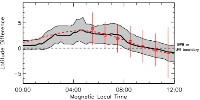
Fig. 6. The black bold line and shaded grey region represent the
spa-tial variation of the median and quartile range, respectively, of the OCB-SWB latitude difference distributions as presented in Fig. 5a. The red symbols and error bars represent the spatial variation of the OCB-UVI latitude differences measured by Carbary et al. (2003). The red dashed line represents the low-order harmonic expansion fit applied to their results by Carbary et al. (2003). The dashed hor-izontal line at zero difference represents the location of the SWB or the UVI poleward boundary.
The high spectral width occurs because the different compo-nents of these spectra are not resolved by the fitACF analysis process, which assumes that backscatter from a single range gate cell is dominated by a single spectral peak.
The spatial distribution of these two classes of spectra in the polar ionospheres shows that they are not randomly distributed in space (Huber and Sofko, 2000; Andr´e et al., 2002). Significant spatial differences are also seen in the variation of the mean and median spectral width values with latitude and MLT (Villain et al., 2002; Chisham and Free-man, 2004), the preferred location for multi-component spec-tra matching the largest specspec-tral width values. This spatial organisation suggests that the origin of high spectral width values is related primarily to physical processes rather than instrumental and/or propagation effects. Candidate processes include the variability within the large-scale ionospheric con-vection pattern (Andr´e et al., 2002; Villain et al., 2002), smaller-scale vortical convection structures generated by fil-amentary Field-Aligned Currents (FACs) (Schiffler et al., 1997; Huber and Sofko, 2000), intense particle precipitation (Baker et al., 1995; Ponomarenko and Waters, 2003) which can result in strong spatial and temporal non-uniformity in ionospheric irregularities, and low-frequency (∼0.01–10 Hz) waves (Andr´e et al., 1999, 2000a; Hosokawa et al., 2004; Wright et al., 2004). However, the extent of the contribution of these different processes in enhancing the Doppler spec-tral width is still unclear.
4.2 Convection variability and spectral width
The level of turbulence/variability in the convection electric field maximises in the cusp and is high in regions where the electric field is high, i.e. in the auroral regions and the polar cap, close to the OCB. If we assume that high spec-tral width is caused by this spatiotemporal variability of the ionospheric electric field then we would expect high
spec-tral width near the OCB, gradually decreasing towards higher and lower latitudes. This is similar to the spatial distribution of spectral width poleward of the OCB (Villain et al., 2002), but low spectral width values are typically observed immedi-ately equatorward of the OCB. Hence, we need to consider an additional factor which quashes the potentially high spectral width values which should occur immediately equatorward of the OCB. So we need to ask whether our observations sug-gest any other factors that are influencing the spectral width?
4.3 Auroral emissions and spectral width
Carbary et al. (2003) showed that the poleward boundary of auroral emissions in the Lyman-Birge-Hopfield “Long” (LBHL) range (∼170 nm) measured by the UVI on the Polar satellite, was a good proxy for the OCB at most MLTs, ex-cept in the early morning sector (∼00:00–09:00 MLT) where the OCB was located ∼2◦–3◦poleward of the UVI proxy.
In Fig. 6 we compare the MLT variation of the median of the OCB-SWB offset (black line), as previously presented in Fig. 5a , with the results of the OCB-UVI poleward bound-ary offsets measured by Carbbound-ary et al. (2003) (red symbols and error bars). The red dashed line is a low-order harmonic expansion fit applied to their data by Carbary et al. (2003). Fig. 6 shows that there is excellent agreement between the two sets of observations. Thus, the poleward edge of the LBHL auroral oval has the same statistical relationship to the OCB as does the SWB. This suggests that the SWB is co-located with the poleward boundary of the LBHL auroral oval.
This is supported by the case study of Wild et al. (2004) in which the SWB, the OCB, and the poleward boundary of the LBH aurora were identified simultaneously in the dawn sec-tor. Using the Wideband Imaging Camera (WIC) on board the IMAGE spacecraft, which measures emissions predom-inantly from the LBH-band (140–180 nm) that includes the LBHL range of the Polar UVI instrument (164–178 nm), the poleward boundary of the LBH aurora was located a few de-grees equatorward of the OCB identified from Cluster space-craft measurements, consistent with the results of Carbary et al. (2003). The SWB identified from SuperDARN radar data was located on the poleward side of the WIC peak (for most of the interval studied), also some degrees equatorward of the OCB, consistent with our results.
However, we must be careful not to generalise these rela-tionships to all poleward auroral emission boundaries. In the Wild et al. (2004) study, the poleward boundary of auroral emissions in the 130–140 nm range, measured by the Spec-trographic Imager at 135.6 nm (SI-13), was poleward of the SWB and co-located with the OCB, the SI-13 emissions be-ing observed across a much larger latitudinal range than the LBH emissions. They concluded that, in the dawn sector, neither the poleward edge of the wide band LBH emission (140–180 nm), nor the SWB, were trustworthy indicators of the OCB location, whereas the narrow band UV emissions in the 130–140 nm range provided a more reliable proxy.
4.4 Electron precipitation and spectral width
Our results, combined with those of Carbary et al. (2003) and Wild et al. (2004), present a consistent picture that the SWB matches closely with the poleward boundary of the au-roral oval measured in the LBHL range. This boundary is approximately co-located with the OCB in all MLT regions except the 02:00–08:00 MLT region. The intensity of LBHL emissions is approximately proportional to the energy flux of precipitating electrons (Germany et al., 1997; Carbary et al., 2004) and varies very little with the average energy of the electrons (Germany et al., 1994). Hence, the correlation be-tween spectral width and LBHL auroral emission boundaries would imply that, statistically, regions of high spectral width correspond to regions of low electron energy flux and that regions of low spectral width correspond to regions of high electron energy flux. This anti-correlation is opposite to the suggestion that intense particle precipitation increases spec-tral width by enhancing the spatial and temporal inhomo-geneity of F-region plasma irregularities (Baker et al., 1995; Ponomarenko and Waters, 2003), at least in the statistically-averaged sense.
Elphinstone et al. (1992) presented a summary of the ranges of values of electron energy flux expected in differ-ent ionospheric precipitation regions. Both the CPS and BPS regions, which are located on closed field lines, are typically characterised by large electron energy fluxes. Conversely, the cusp, mantle and polar rain regions, which are located on open field lines, are typically characterised by low electron energy fluxes. This would then explain the typical pattern of high spectral width in open field line regions and low spec-tral width in closed field line regions that is observed across much of the polar ionosphere, as shown in this paper and Chisham et al. (2004). The LLBL represents a difficult re-gion to define as the electron energy fluxes can be low or high in this region and hence, the LLBL could be characterised by either low or high spectral width. Baker et al. (1995) associ-ated the LLBL with low spectral width values. We suggest that these low spectral width values are associated with high electron energy fluxes on closed LLBL field lines but that there are occasional intrusions of open LLBL field lines with low electron energy flux and high spectral width, associated with reconnection transients (Pinnock et al., 1995).
Statistical studies of the variation of electron energy flux across the polar ionospheres have shown that the energy flux peaks at lower latitudes in the post-midnight/dawn sector than in other sectors (Hardy et al., 1985), and some distance equatorward of the OCB (Sotirelis and Newell, 2000). This would be consistent with the offset observed between the SWB and the OCB in this region.
4.5 Conductivity and spectral width
Having established an anti-correlation between spectral width and precipitating electron energy flux, our final ques-tion is why the high electron energy fluxes lead to a reduc-tion in the measured spectral width values. Germany et al.
(1994) showed that ionospheric conductivity increases with increasing incident electron energy flux. Weimer et al. (1985) showed that small-scale electric field structures do not map very efficiently to low altitudes in the auroral zone iono-sphere and argued that the damping of this variability is pro-portional to ionospheric conductivity; smaller-scale electric field structures mapping better along the magnetic field to lower altitudes in regions of lower conductivity. Hence, it is probable that high electron energy flux quashes much of the small-scale variability in the ionospheric electric field through increased conductivity (Parkinson et al., 2004). 4.6 A simple spectral width model
Thus, we argue that the combination of two factors may ex-plain the spatial distribution of spectral width values in the polar ionospheres. The small-scale spatiotemporal structure of the convection electric field leads to an enhancement of spectral width in regions close to the OCB whereas increases in ionospheric conductivity (relating to the level of incident electron energy flux) lead to a reduction in spectral width in regions just equatorward of the OCB. This simple model for explaining spectral width variations in the ionosphere could be tested by an in-depth statistical comparison of the phe-nomena involved.
5 Conclusions and summary
By correlating 5 years of SWBs measured by the Super-DARN HF radar network with PPBs measured by the DMSP spacecraft, we have determined a clear statistical picture which describes how the SWB relates to the OCB in the morning sector ionosphere. The SWB represents a good proxy for the OCB close to midnight (00:00–02:00 MLT) and noon (08:00–12:00 MLT) but is located some distance (∼2◦–4◦) equatorward of the OCB across the rest of the
morning sector ionosphere (02:00–08:00 MLT). Hence, we cannot reliably use the SWB as a proxy for the OCB in this MLT region. We have argued that the SWB correlates well with the poleward boundary of UV auroral emissions in the LBHL emission range and hence, that spectral width is in-versely correlated with the level of incident electron energy flux. Further statistical studies comparing the variations of other possible contributing factors with variations in Doppler spectral width are needed before a definitive statement can be made about the origin of high spectral width in HF radar backscatter.
Acknowledgements. We would like to thank the principal inves-tigators of the SuperDARN radars used in this study: G. Sofko (Saskatoon) and M. Pinnock (Halley). CUTLASS is supported by the PPARC (UK), the Swedish Institute for Space Physics, Upp-sala, and the FMI, Helsinki (Finland). Support for the Goose Bay and Kapuskasing radars is provided in part by the NSF (USA), and in part by NASA (USA). Support for the Saskatoon radar is pro-vided by NSERC (Canada). The Halley radar was developed under funding from the NERC (UK) and the NSF (USA). Operations are supported by the NERC (UK). The DMSP particle detectors were
designed by D. Hardy of AFRL (USA), and data obtained from JHU/APL (USA). We thank D. Hardy, F. Rich, and P. T. Newell for their use. During part of the preparation of this paper ML was supported by the Institute for Advanced Study, La Trobe University, Melbourne, Australia. The authors would like to thank Mike Pin-nock and Alan Rodger for helpful discussions.
Topical Editor in chief thanks G. Blanchard and W. Bristow for their help in evaluating this paper.
References
Andr´e, R., Pinnock, M., and Rodger, A. S.: On the SuperDARN autocorrelation function observed in the ionospheric cusp, Geo-phys. Res. Lett., 26, 3353–3356, 1999.
Andr´e, R., Pinnock, M., and Rodger, A. S.: Identification of the low-altitude cusp by Super Dual Auroral Radar Network radars: A physical explanation for the empirically derived signature, J. Geophys. Res., 105, 27 081–27 093, 2000a.
Andr´e, R., Pinnock, M., Villain, J.-P., and Hanuise, C.: On the fac-tors conditioning the Doppler spectral width determined from SuperDARN HF radars, Int. J. Geomagn. Aeron., 2, 77–86, 2000b.
Andr´e, R., Pinnock, M., Villain, J.-P., and Hanuise, C.: Influence of magnetospheric processes on winter HF radar spectra character-istics, Ann. Geophys., 20, 1783–1793, 2002,
SRef-ID: 1432-0576/ag/2002-20-1783.
Baker, K. B., Dudeney, J. R., Greenwald, R. A., Pinnock, M., Newell, P. T., Rodger, A. S., Mattin, N., and Meng, C.-I.: HF radar signatures of the cusp and low-latitude boundary layer, J. Geophys. Res., 100, 7671–7695, 1995.
Baker, K. B., Rodger, A. S., and Lu, G.: HF-radar observations of the dayside magnetic merging rate: A Geospace Environment Modeling boundary layer campaign study, J. Geophys. Res., 102, 9603–9617, 1997.
Baker, J. B., Clauer, C. R., Ridley, A. J., Papitashvili, V. O., Brit-tnacher, M. J., and Newell, P. T.: The nightside poleward bound-ary of the auroral oval as seen by DMSP and the Ultraviolet Im-ager, J. Geophys. Res., 105, 21 267–21 280, 2000.
Blanchard, G. T., Lyons, L. R., Samson, J. C., and Rich, F. J.: Locat-ing the polar cap boundary from observations of 6300 ˚A auroral emission, J. Geophys. Res., 100, 7855–7862, 1995.
Blanchard, G. T., Lyons, L. R., de la Beaujardi`ere, O., Doe, R. A., and Mendillo, M.: Measurement of the magnetotail reconnection rate, J. Geophys. Res., 101, 15 265–15 276, 1996.
Blanchard, G. T., Lyons, L. R., and Samson, J. C.: Accuracy of using 6300 ˚A auroral emission to identify the magnetic separatrix on the nightside of the earth, J. Geophys. Res., 102, 9697–9703, 1997.
Blanchard, G. T., Ellington, C. L., Lyons, L. R., and Rich, F. J.: In-coherent scatter radar identification of the dayside magnetic sep-aratrix and measurement of magnetic reconnection, J. Geophys. Res., 106, 8185–8195, 2001.
Brittnacher, M., Fillingim, M., Parks, G., Germany, G., and Spann, J.: Polar cap area and boundary motion during substorms, J. Geo-phys. Res., 104, 12 251–12 262, 1999.
Carbary, J. F., Sotirelis, T., Newell, P. T., and Meng, C.-I.: Auro-ral boundary correlations between UVI and DMSP, J. Geophys. Res., 108, 1018, doi:10.1029/2002JA009378, 2003.
Carbary, J. F., Sotirelis, T., Newell, P. T., and Meng, C.-I.: Cor-relation of LBH intensities with precipitating particle energies,
Geophys. Res. Lett., 31, L13801, doi:10.1029/2004GL019888, 2004.
Chisham, G., Pinnock, M., and Rodger, A. S.: The response of the HF radar spectral width boundary to a switch in the IMF By direction: Ionospheric consequences of transient dayside recon-nection? J. Geophys. Res., 106, 191–202, 2001.
Chisham, G. and Pinnock, M.: Assessing the contamination of Su-perDARN global convection maps by non-F-region backscatter, Ann. Geophys., 20, 13–28, 2002,
SRef-ID: 1432-0576/ag/2002-20-13.
Chisham, G., Pinnock, M., Coleman, I. J., Hairston, M. R., and Walker, A. D. M: An unusual geometry of the ionospheric sig-nature of the cusp: Implications for magnetopause merging sites, Ann. Geophys., 20, 29–40, 2002,
SRef-ID: 1432-0576/ag/2002-20-29.
Chisham, G. and Freeman, M. P.: A technique for accurately deter-mining the cusp-region polar cap boundary using SuperDARN HF radar measurements, Ann. Geophys., 21, 983–996, 2003,
SRef-ID: 1432-0576/ag/2003-21-983.
Chisham, G., Freeman, M. P., and Sotirelis, T.: A statistical comison of SuperDARN spectral width boundaries and DMSP par-ticle precipitation boundaries in the nightside ionosphere, Geo-phys. Res. Lett., 31, L02804, doi:10.1029/2003GL019074, 2004. Chisham, G. and Freeman, M. P.: An investigation of latitudinal transitions in the SuperDARN Doppler spectral width parameter at different magnetic local times, Ann. Geophys., 22, 1187–1202, 2004,
SRef-ID: 1432-0576/ag/2004-22-1187.
Cowley, S. W. H. and Lockwood, M.: Excitation and decay of so-lar wind-driven flows in the magnetosphere-ionosphere system, Ann. Geophys., 10, 103–115, 1992.
de la Beaujardi`ere, O., Lyons, L. R., Ruohoniemi, J. M., Friis-Christensen, E., Danielsen, C., Rich, F. J., and Newell, P. T.: Quiet-time intensifications along the poleward auroral boundary near midnight, J. Geophys. Res., 99, 287–298, 1994.
Elphinstone, R. D., Murphree, J. S., Hearn, D. J., Cogger, L. L., Newell, P. T., and Vo, H.: Viking observations of the UV dayside aurora and their relationship to DMSP particle boundary defini-tions, Ann. Geophys., 10, 815–826, 1992.
Freeman, M. P. and Chisham, G.: On the probability distribu-tions of SuperDARN Doppler spectral width measurements in-side and outin-side the cusp, Geophys. Res. Lett., 31, L22802, doi:10.1029/2004GL020923, 2004.
Germany, G. A., Torr, D. G., Richards, P. G., Torr, M. R., and John, S.: Determination of ionospheric conductivities from FUV auro-ral emissions, J. Geophys. Res., 99, 23 297–23 305, 1994. Germany, G. A., Parks, G. K., Brittnacher, M., Cumnock, J.,
Lum-merzheim, D., Spann, J. F., Chen, L., Richards, P. G., and Rich, F. J.: Remote determination of auroral energy characteristics dur-ing substorm activity, Geophys. Res. Lett., 24, 995–998, 1997. Greenwald, R. A., Baker, K. B., Dudeney, J. R., Pinnock, M., Jones,
T. B., Thomas, E. C., Villain, J.-P., Cerisier, J.-C., Senior, C., Hanuise, C., Hunsucker, R. D., Sofko, G., Koehler, J., Nielsen, E., Pellinen, R., Walker, A. D. M., Sato, N., and Yamagishi, H.: DARN/SuperDARN: A global view of the dynamics of high-latitude convection, Space Sci. Rev., 71, 761–796, 1995. Hardy, D. A., Gussenhoven, M. S., and Holeman, E.: A
statisti-cal model of auroral electron precipitation, J. Geophys. Res., 90, 4229–4248, 1985.
Hosokawa, K., Yamashita, S., Stauning, P., Sato, N., Yukimatu, A. S., and Iyemori, T.: Origin of the SuperDARN broad Doppler spectra: simultaneous observation with Oersted satellite
magne-tometer, Ann. Geophys., 22, 159–168, 2004,
SRef-ID: 1432-0576/ag/2004-22-159.
Huber, M. and Sofko, G.: Small-scale vortices in the high-latitude F region, J. Geophys. Res., 105, 20 885–20 897, 2000.
Kauristie, K., Weygand, J., Pulkkinen, T. I., Murphree, J. S., and Newell, P. T.: Size of the auroral oval: UV ovals and precipitation boundaries compared, J. Geophys. Res., 104, 2321–2331, 1999. Milan, S. E., Lester, M., Cowley, S. W. H., Moen, J., Sandholt,
P. E., and Owen, C. J.: Meridian-scanning photometer, coherent HF radar, and magnetometer observations of the cusp: a case study, Ann. Geophys., 17, 159–172, 1999,
SRef-ID: 1432-0576/ag/1999-17-159.
Milan, S. E. and Lester, M.: Interhemispheric differences in the HF radar signature of the cusp region: A review through the study of a case example, Adv. Polar Upper Atmos. Res., 15, 159–177, 2001.
Milan, S. E., Lester, M., Cowley, S. W. H., Oksavik, K., Brittnacher, M., Greenwald, R. A., Sofko, G., and Villain, J.-P.: Variations in the polar cap area during two substorm cycles, Ann. Geophys., 21, 1121–1140, 2003,
SRef-ID: 1432-0576/ag/2003-21-1121.
Milan, S. E., Cowley, S. W. H., Lester, M., Wright, D. M., Slavin, J. A., Fillingim, M., Carlson, C. W., and Singer, H. J.: Re-sponse of the magnetotail to changes in the open flux con-tent of the magnetosphere, J. Geophys. Res., 109, A04220, doi:10.1029/2003JA010350, 2004.
Newell, P. T., Burke, W. J., Sanchez, E. R., Meng, C.-I., Greenspan, M. E., and Clauer, C. R.: The low-latitude boundary layer and the boundary plasma sheet at low altitude: Prenoon precipitation regions and convection reversal boundaries, J. Geophys. Res., 96, 21 013–21 023, 1991.
Newell, P. T. and Meng, C.-I.: Mapping the dayside ionosphere to the magnetopause according to particle precipitation events, Geophys. Res. Lett., 19, 609–612, 1992.
Newell, P. T., Feldstein, Y. I., Galperin, Y. I., and Meng, C.-I.: Morphology of nightside precipitation, J. Geophys. Res., 101, 10 737–10 748, 1996a.
Newell, P. T., Feldstein, Y. I., Galperin, Y. I., and Meng, C.-I.: Cor-rection to “Morphology of nightside precipitation”, J. Geophys. Res., 101, 17 419–17 421, 1996b.
Parkinson, M. L., Chisham, G., Pinnock, M., Dyson, P. L., and Devlin, J. C.: Magnetic local time, substorm, and particle precipitation-related variations in the behaviour of SuperDARN Doppler spectral widths, Ann. Geophys., 22, 4103–4122, 2004,
SRef-ID: 1432-0576/ag/2004-22-4103.
Pinnock, M., Rodger, A. S., Dudeney, J. R., Rich, F., and Baker, K. B.: High spatial and temporal resolution observations of the ionospheric cusps, Ann. Geophys., 13, 919–925, 1995,
SRef-ID: 1432-0576/ag/1995-13-919.
Pinnock, M., Chisham, G., Coleman, I. J., Freeman, M. P., Hairston, M., and Villain, J.-P.: The location and rate of dayside recon-nection during an interval of southward interplanetary magnetic field, Ann. Geophys., 21, 1467–1482, 2003,
SRef-ID: 1432-0576/ag/2003-21-1467.
Ponomarenko, P. V. and Waters, C. L.: The role of Pc1-2 waves in spectral broadening of SuperDARN echoes from high latitudes, Geophys. Res. Lett., 30, 1122, doi:10.1029/2002GL016333, 2003.
Sandholt, P. E., Farrugia, C. J., Øieroset, M., Stauning, P., and Denig, W. F.: Auroral activity associated with unsteady magne-tospheric erosion: Observations on 18 December 1990, J. Geo-phys. Res., 103, 2309–2317, 1998.
Schiffler, A., Sofko, G., Newell, P. T., and Greenwald, R. A.: Map-ping the outer LLBL with SuperDARN double-peaked spectra, Geophys. Res. Lett., 24, 3149–3152, 1997.
Siscoe, G. L. and Huang, T. S.: Polar cap inflation and deflation, J. Geophys. Res., 90, 543–547, 1985.
Sotirelis, T. and Newell, P. T.: Boundary-oriented electron precipi-tation model, J. Geophys. Res., 105, 18 655–18 673, 2000. Villain, J.-P., Andr´e, R., Pinnock, M., Greenwald, R. A., and
Hanuise, C.: A statistical study of the Doppler spectral width of high-latitude ionospheric F-region echoes recorded with Su-perDARN coherent HF radars, Ann. Geophys., 20, 1769–1781, 2002,
SRef-ID: 1432-0576/ag/2002-20-1769.
Weimer, D. R., Goertz, C. K., Gurnett, D. A., Maynard, N. C., and Burch, J. L.: Auroral-zone electric fields from DE-1 and DE-2 at magnetic conjunctions, J. Geophys. Res., 90, 7479–7494, 1985. Wild, J. A., Milan, S. E., Owen, C. J., Bosqued, J. M., Lester, M.,
Wright, D. M., Frey, H., Carlson, C. W., Fazakerley, A. N., and R`eme, H.: The location of the open-closed magnetic field line boundary in the dawn sector auroral ionosphere, Ann. Geophys., 22, 3625–3639, 2004,
SRef-ID: 1432-0576/ag/2004-22-3625.
Woodfield, E. E., Davies, J. A., Eglitis, P., and Lester, M.: A case study of HF radar spectral width in the post midnight magnetic local time sector and its relationship to the polar cap boundary, Ann. Geophys., 20, 501–509, 2002.
SRef-ID: 1432-0576/ag/2002-20-501.
Wright, D. M., Yeoman, T. K., Baddeley, L. J., Davies, J. A., Dhillon, R. S., Lester, M., Milan, S. E., and Woodfield, E. E.: High resolution observations of spectral width features associ-ated with ULF wave signatures in artificial HF radar backscatter, Ann. Geophys., 22, 169–182, 2004,
SRef-ID: 1432-0576/ag/2004-22-169.
Yeoman, T. K., Wright, D. M., Stocker, A. J., and Jones, T. B.: An evaluation of range accuracy in the Super Dual Auroral Radar Network over-the-horizon HF radar systems, Radio Sci., 36, 801–813, 2001.