HAL Id: hal-00317095
https://hal.archives-ouvertes.fr/hal-00317095
Submitted on 1 Jan 2003
HAL is a multi-disciplinary open access
archive for the deposit and dissemination of
sci-entific research documents, whether they are
pub-lished or not. The documents may come from
teaching and research institutions in France or
abroad, or from public or private research centers.
L’archive ouverte pluridisciplinaire HAL, est
destinée au dépôt et à la diffusion de documents
scientifiques de niveau recherche, publiés ou non,
émanant des établissements d’enseignement et de
recherche français ou étrangers, des laboratoires
publics ou privés.
approaching solar activity maximum: interpreting
Ulysses observations using a global MHD model
P. Riley, Z. Miki?, J. A. Linker
To cite this version:
P. Riley, Z. Miki?, J. A. Linker. Dynamical evolution of the inner heliosphere approaching solar
ac-tivity maximum: interpreting Ulysses observations using a global MHD model. Annales Geophysicae,
European Geosciences Union, 2003, 21 (6), pp.1347-1357. �hal-00317095�
Annales
Geophysicae
Dynamical evolution of the inner heliosphere approaching solar
activity maximum: interpreting Ulysses observations using a global
MHD model
P. Riley, Z. Miki´c, and J. A. Linker
Science Applications International Corporation, 10260 Campus Point Dr., San Diego, CA 92121, USA Received: 31 October 2002 – Revised: 2 February 2003 – Accepted: 7 February 2003
Abstract. In this study we describe a series of MHD
simu-lations covering the time period from 12 January 1999 to 19 September 2001 (Carrington Rotation 1945 to 1980). This interval coincided with: (1) the Sun’s approach toward so-lar maximum; and (2) Ulysses’ second descent to the south-ern polar regions, rapid latitude scan, and arrival into the northern polar regions. We focus on the evolution of several key parameters during this time, including the photospheric magnetic field, the computed coronal hole boundaries, the computed velocity profile near the Sun, and the plasma and magnetic field parameters at the location of Ulysses. The model results provide a global context for interpreting the often complex in situ measurements. We also present a heuristic explanation of stream dynamics to describe the morphology of interaction regions at solar maximum and contrast it with the picture that resulted from Ulysses’ first orbit, which occurred during more quiescent solar condi-tions. The simulation results described here are available at: http://sun.saic.com.
Key words. Interplanetary physics (Interplanetary magnetic
fields; solar wind plasma; sources of the solar wind)
1 Introduction
Beyond ∼10 solar radii (RS), solar material streams away from the Sun along roughly radial trajectories. A combina-tion of temporal variacombina-tions at the Sun, together with the ro-tation of the Sun, leads to parcels of plasma with different plasma and magnetic properties becoming radially aligned: faster material overtaking slower material leads to a com-pression front, while slower material being outrun by faster material leads to a rarefaction region, or expansion wave (Sarabhai, 1963). When the flow pattern at the Sun does not vary considerably during a solar rotation (such as during so-lar minimum), the so-large-scale compressive structures created by the interaction of these streams are fixed in a frame
coro-Correspondence to: P. Riley ([email protected])
tating with the Sun, and they are known as corotating inter-action regions (CIRs) (Smith and Wolfe, 1976). When the difference in speed between the slow and fast streams is suf-ficiently large, a pair of shocks may form bounding the CIR (Pizzo, 1985).
During its initial voyage out of the ecliptic plane, Ulysses observed a systematic orientation of the CIRs it encountered (Gosling et al., 1993, 1995; Riley et al., 1996; Gonzalez-Esparza and Smith, 1997). These interaction regions were observed from January 1992 to October 1993, correspond-ing to the declincorrespond-ing phase of solar cycle 22. In the azimuthal (φ) plane their outward normals were tilted westward (i.e. into the direction of planetary motion). This was to be ex-pected, as the interaction regions aligned themselves roughly along the direction of the Parker spiral. In the meridional plane (θ ) their outward normals were tilted toward the helio-graphic equator. These results were supported by numerical MHD simulations (Pizzo, 1994) which suggested that these orientations were a natural consequence of the tilt of the solar magnetic dipole axis relative to the solar rotation axis. This pattern of tilts was once again observed during Ulysses’ so-called “rapid latitude scan” (Gosling et al., 1995) and, most recently, as Ulysses descended from the northen polar re-gions to the equator (Gosling et al, 1997; Mc Comas et al., 1998).
Previous solar wind models have yielded considerable in-sight into the dynamical processes that shape the structure of the heliosphere. The large-scale, time-stationary struc-ture of the heliosphere under an idealized tilted-dipole ge-ometry has been studied in detail by V. J. Pizzo (e.g. Pizzo, 1991; Pizzo and Gosling, 1994, and references therein). At an inner boundary of 32 RS a flow pattern was constructed consisting of a slow, dense flow about a heliomagnetic equa-tor that was tilted by a specified amount relative to the rota-tional axis. Similar simulations were used by Pizzo (1994) to interpret Ulysses observations at mid-heliographic latitudes, where it was found that CIR-associated reverse shocks per-sist to much higher latitudes than CIR-associated forward shocks. These results suggested that the tilted-dipole
geom-etry at the inner boundary strongly drives the position and orientation of the CIRs and their associated shocks. In par-ticular, under moderately low solar activity conditions, CIRs and shock outward normals are tilted toward the equator in both hemispheres. Thus, in the ecliptic plane a spacecraft samples alternating tilts as it passes through a predominantly Northern Hemispheric CIR and, subsequently, a predomi-nantly Southern Hemispheric CIR. Moreover, the strongest interactions take place away from the ecliptic plane, at lati-tudes roughly equal to the tilt of the solar dipole relative to the rotation axis.
Wang and Sheeley (1990) exploited an empirical relation-ship between solar wind speed and coronal flux tube expan-sion (Levine et al., 1977) to predict solar wind speed at 1 AU and beyond. They found that coronal flux tubes that expand more slowly correlate with faster asymptotic speed along that flux tube. Using this relationship, they predicted the types of wind speed patterns that Ulysses would be expected to see during its second solar orbit (Wang and Sheeley, 1997). In particular, they predicted that the ascending phase of the so-lar cycle would be dominated by recurrent (28–29 day pe-riodicity), high-speed streams originating from high-latitude extensions of polar coronal holes. Approaching solar max-imum, however, persistent high-speed streams would disap-pear, only to be replaced by low-speed wind at all latitudes. Finally, at solar maximum (or, more specifically, at the time that the polar field reverses), very fast episodic polar jets would be generated as active region fields migrated toward the solar poles.
The data utilized in this study derive from the Solar Wind Observations Over the Poles of the Sun (SWOOPS) ion sen-sor (Bame et al., 1992) and the magnetic field investigation (Balogh, 1992) on board the Ulysses spacecraft. The plasma moments have a typical resolution of 4–8 min while the mag-netic field measurements have a resolution of 1–2 s. All data presented here, however, have been averaged over 1 hour.
The purpose of this report is twofold. First, we describe a series of MHD simulations covering approximately 3 years during the late ascending phase of the solar cycle and through solar maximum and use them to interpret Ulysses in situ ob-servations. Second, we present a simple explanation for both the observed and modeled stream structure at solar maxi-mum, and contrast it with solar minimum conditions. The report is structured as follows. In Sect. 2 we describe the basic features and approximations inherent to the model. In Sect. 3 was discuss the properties and evolution of the so-lar wind as seen by Ulysses during the time period from 12 January 1999 to 19 September 2001. In Sect. 4 we describe the global evolution of the inner heliosphere as inferred from the MHD simulations for the same time period. We explore two specific intervals in more detail in Sect. 5 to highlight the differences in stream structure between solar minimum and maximum. Finally, in Sect. 6 we summarize the main points of the study, address some of the limitations and sources of errors in the simulations, and discuss possible areas for future studies.
2 Description of the model
We use a three-dimensional, time-dependent MHD model, driven by the observed line-of-sight photospheric magnetic field to model the structure of the inner heliosphere (1 RS to 5 AU). The details of the algorithm have been discussed by Miki´c et al. (1999) and Linker et al. (1999) and its extension from the solar corona to the inner heliosphere is discussed by Riley et al. (2001a,b). Briefly speaking, we separate the region of space from 1 RS to 5 AU into two distinct regions: the coronal model, which spans 1 RSto 30 RSand the helio-spheric model, which spans 30 RSto 5 AU. Such an approach is both computationally more efficient and produces a more realistic heliospheric environment.
The heliospheric boundary conditions are specified in the following way:
1. The radial component of the coronal magnetic field at 30 RS is used directly as the inner boundary condition for Br.
2. The speed is computed using the coronal magnetic con-figuration: at 1 RS we set the radial speed to be some value, vslow, at the boundary between open and closed field lines over a width of ∼ 6◦(in a direction normal to the boundary) and smoothly raise it to vfast over ∼ 3◦. We then map this speed profile outward along the open field lines to 30 RS. Although this may appear some-what ad hoc, it is based on the commonly held view that fast wind emanates from within coronal holes and slow wind is associated with the boundary between open and closed fields, as would be the case if closed field lines were sporadically opened, through magnetic reconnec-tion. Such an approach is required because the poly-tropic approximation used in the coronal solution does not yield sufficiently large variations between the slow and fast wind.
3. We assume a momentum flux balance at the inner boundary, which specifies the plasma density.
4. We assume thermal pressure balance, yielding the plasma temperature. Comparisons with in situ observa-tions suggest that this approach is capable of capturing the essential features of the large-scale structure of the inner heliosphere for a variety of solar conditions (Riley et al., 2001a,b).
Riley et al. (2001a) have discussed the approximations of this model in detail. Here we make a few brief remarks. First, we neglect the effect of pickup ions, which are thought to dominate the internal energy of the solar wind beyond 6– 10 AU (Axford, 1973). Thus, we limit our modeling region to ∼5 AU. Second, we neglect the effects of differential rota-tion, which may play a role in connecting high-latitude field lines near the Sun with lower-latitude interaction regions much further away (Fisk, 1996). Third, although our MHD model is time-dependent, we assume that the flow at the in-ner boundary is time-stationary. Thus, the flow at the inin-ner
boundary rotates rigidly with a period of 25.38 days and spa-tial variations are responsible for the generation of dynamic phenomena in the solution. Consequently, our results do not include transient phenomena, such as coronal mass ejections. Finally, the grid resolution necessary to model a region of space spanning 5 AU in radius precludes us from accurately modeling shock waves.
Since the model, as implemented here, is driven by synop-tic maps of the line-of-sight photospheric magnesynop-tic field ob-served at the Kitt Peak observatory, each solution describes an “average” picture for that Carrington rotation. And, while the solution does not contain any transient phenomena, it can be interpreted as the “underlying” solution, assuming that the magnetic configuration responsible for the transient event re-turned to its initial state after eruption. In spite of these limi-tations, even under solar maximum conditions, this approach can produce results that compare favorably with in situ ob-servations (Riley et al., 2002).
3 Ulysses observations
By early 1999, the Ulysses spacecraft had already begun its second excursion from the ecliptic plane toward the sourth-ern polar regions of the Sun. Moving in from 5.19 AU and
−19.6◦ heliographic latitude on 12 January 1999, Ulysses reached a peak southern latitude of −80.2◦ on 23 Novem-ber 2000 (day 328) and then swung rapidly from the south-ern polar regions to the northsouth-ern polar regions, crossing the equator on 17 May 2001 (day 137) at a distance of 1.34 AU and reaching a peak northern latitude of +80.2◦on 11 Oc-tober 2001 (day 284). In this study, we focus on CR1945-CR1980, corresponding to the time period 12 January 1999 to 19 September 2001. Figure 1 summarizes Ulysses’ tra-jectory during this time period (bottom panel), together with speed, proton number density (np, scaled by r2to account for the spherical expansion of the solar wind) and proton temper-ature (Tp, scaled by r to account for the near-adiabatic expan-sion of the solar wind). We see that the majority of solar wind intercepted by Ulysses was relatively slow and variable. In fact, in 1999 and 2000, the wind only exceeded 600 km s−1 a few times. By the time Ulysses had reached ∼60◦N heli-olatitude, substantial intervals of high-speed wind were once again observed (McComas et al., 2002b). A clear transition occurred in August 2001, however, when the spacecraft be-came immersed in high-speed, tenuous, and quescient solar wind, similar to what was observed over both poles during its first orbit. At this point, Ulysses had crossed the solar pole and was back at ∼60◦N heliolatitude. Also of note is that the slowest density and coldest flow occurred during late 2000 and early 2001 when the average speed remained less than 400 km s−1. The structure of the solar wind, as inferred from these plasma measurements, has been discussed in de-tail by McComas et al. (2000, 2002a,b); McComas (2002).
Fig. 1. Ulysses measurements (1-h averages) of solar wind speed,
density, and temperature, together with the spacecraft’s location (ra-dial distance: red, and heliographic latitude: blue) from 12 January 1999 to 19 September 2001.
4 Evolution of the solar wind approaching solar maxi-mum
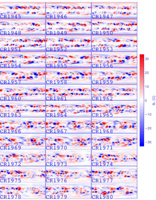
The inputs used to construct the model solutions for CR1945 to CR1980 are shown in Fig. 2, where Carrington longi-tude (0◦–360◦) runs along the x-axis and heliographic lati-tude (−90◦to +90◦) runs along the y-axis. These were de-rived from Kitt Peak measurements of the line-of-sight pho-tospheric magnetic field, and have undergone significant pro-cessing to provide more appropriate boundary conditions for the simulations. Since these inputs are the principal driver of the model, it is worth discussing this method in some de-tail. First, accurate measurements of the polar fields (say above ±70◦) are difficult because of line-of-sight projection effects. Thus, rather than use unreliable data, measurements within 20◦of each pole were replaced by values extrapolated from a two-term Taylor series fit of the axisymmetric compo-nent of the observed field between 14◦and 28◦of the poles. Second, any small residual monopolar component to the field was subtracted out. Third, the data were interpolated to the resolution used in the simulation, while preserving the mag-netic flux in the interpolation. Fourth, a longitudinal filter of the form e−(0.7m/mmax)8 was applied, where m
max specifies the mode that is attenuated to 95% of its original amplitude,
Fig. 2. Radial magnetic field at the photosphere for CR1945 to CR1980, derived from Kitt Peak synoptic maps.
and modes with m smaller than mmaxare not attenuated ap-preciably. For these simulations, mmax=9 was chosen. The resulting values provide the radial component of the mag-netic field at our inner boundary, Br0. We caution that a comparison of these results with the original Kitt Peak mag-netograms reveal some significant differences (Linker et al., 1999). In particular, the small-scale “peppered” appearance is replaced with large-scale bipole regions, preferentially se-lected by the particular value of mmaxchosen. On the other hand, the large-scale structure of the data is well preserved.
Scanning the panels in Fig. 2, we note that, in general, there is significant evolution from one rotation to the next. However, many features persist for several rotations. The most striking trend, however, is the reversal of the polar fields during this time span. Initially, the polar fields are outward (red) in the Northern Hemisphere and inward (blue) in the Southern Hemisphere. By the end of the time period they
are outward in the Southern Hemisphere and inward in the Northern Hemisphere. The mid-point likely occurred be-tween CR1969 and CR1973, or 27 October 2000–13 March 2001 (inferred by saturating the colors in Fig. 2).
The specification of the remaining boundary conditions, as well as the initial condition for the magnetofluid variables, has been described by Linker et al. (1999) and are not re-peated here. Given this initial state and boundary conditions the MHD equations are then integrated forward in time until a steady state equilibrium is achieved. This procedure was repeated for each Carrington rotation until a database of 36 coronal solutions was obtained.
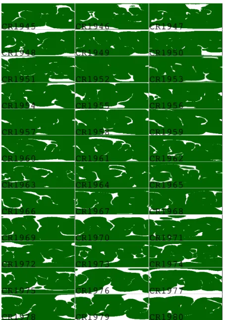
These solutions allow us to compute coronal hole bound-aries, i.e. the boundary between open and closed magnetic field lines, by tracing along magnetic field lines and deter-mining whether they are open (i.e. extend out through the outer boundary of the coronal solution) or are closed (i.e.
re-Fig. 3. Computed coronal hole boundaries for CR1945 to CR1980. Green indicates regions of closed magnetic fields and white indicates
regions of open magnetic fields (i.e. coronal holes).
turn back to the surface of the Sun). We emphasize that these computed boundaries are not necessarily the same as coronal hole boundaries computed from Kitt Peak He I 1083 nm ob-servations. In fact, they are typically a superset. This may signify an error in the modeling, or may suggest that the ob-servations do not always identify the boundaries well. We should also mention that there is an implicit, although rea-sonable assumption that coronal holes are in fact defined by open field lines.
In Fig. 3 we summarize the computed coronal hole bound-aries. The large-scale polar coronal holes that were consis-tently present during Ulysses’ first orbit are gone, replaced instead by smaller coronal holes located at essentially all he-liographic latitudes. Initially, a small southern coronal hole is present for 4 rotations or so. We should be cautious, however, about over-interpreting results at the highest heliolatitudes,
since our accuracy there is the poorest. A fairly substantial northern coronal hole was present in rotations 1969–1971, and there is an indication that polar coronal holes are again returning toward the end of the time period. The overwhelm-ing feature of these maps, however, is how small the fraction of the solar surface is that is covered by coronal holes. Typi-cally, they account for only ∼6%. Comparison of Fig. 3 with Fig. 2 highlights the importance of MHD (or potential field source surface) models in revealing the magnetic field struc-ture of the corona. It would be difficult, if not impossible, to infer the topology of magnetic field lines and/or the lo-cation or coronal holes based only on the photospheric field data. A detailed comparison of these results with Kitt Peak He I 1083 nm observations, while clearly of importance, is beyond the scope of the present study.
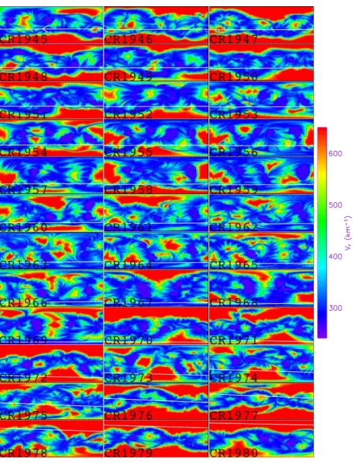
Fig. 4. Computed radial velocities for CR1945 to CR1980. The solid line in each panel indicates Ulysses’ mapped trajectory along this
spherical shell.
(2001a,b), the coronal solutions are used to calculate the boundary conditions for the heliospheric portion of the model at 30 RS. The radial component of the magnetic field is used directly, while the velocity, density, and temperature are cal-culated in a somewhat more ad hoc way. The computed speeds at 30 RSare shown in Fig. 4. Ulysses’ trajectory has also been projected back to the Sun for each Carrington ro-tation and is displayed as a white line. Time runs in the op-posite sense to longitude, and so it increases from right to left.
The flow speed of the solar wind at 30 RSis not typically considered to be a fundamental parameter, since measure-ments in this region are difficult to make and hence sparse. Nevertheless, they are an excellent tool for interpreting the global context of in situ measurements. At this distance, all
super-radial expansion has occurred and the flow is essen-tially radial, yet no stream dynamics have taken place to any significant extent, complicating the flow pattern. Thus, we have the potential to resolve such questions as to whether the presence of an intermediate-speed stream (say, 600 km s−1) was the result of the spacecraft grazing the edge of a substan-tial coronal hole, or intercepting a smaller high-speed stream that has decelerated, via the interaction with slow solar wind during its passage to the spacecraft (stream attenuation). We are currently studying these simulations in greater detail to assess how well the computed stream structure matches ob-servations at Ulysses, WIND, and ACE. Previously (Riley et al., 2001a,b), we have shown that they can reproduce the essential stream structure patterns, particularly at solar mini-mum. We realize, however, that at solar maximum, temporal
variations at the Sun will undoubtedly lead to streams that cannot be modeled with our synoptic solutions and we do not expect to match the observations all of the time.
There is a clear evolutionary trend to the stream structure shown in Fig. 4. Initially, a pair of high speed streams em-anate from both poles. By CR1952 the northern high-speed stream has disappeared and by CR1959, the southern high speed stream is gone. Ulysses at this time was traveling from low latitudes toward the southern polar regions, and, as can be seen in Fig. 4, chased the receding coronal hole with-out ever becoming immersed within in. Between CR1959 and CR1968 only smaller high-speed streams were present. Ulysses intercepted them, but by the time they had pushed their way out to the location of the spacecraft, they were re-duced to a speed of less than 600 km s−1. During rotations CR1969 – CR1972 a fairly substantial high-speed stream was present over the northern polar region, but Ulysses, still being in the Southern Hemisphere, had no direct knowledge of it. However, by the time Ulysses had reached equatorial regions during its rapid latitude scan, both the northern and south-ern regions were developing polar coronal holes and hence high-speed flow. Ulysses intercepted the southern edge of the northern polar stream in CR1978, and became completely immersed in it the following rotation.
Although we have emphasized the high-speed streams in our discussion, we could have equally well described Ulysses’ journey relative to the slower, more variable wind. During a few rotations, such as CR1947 and CR1976, we see the “tilted-dipole” picture, as suggested by the ideal-ized streams modeled by Pizzo (1994), where the slow wind is confined to a constant-width, sinusoidally-varying profile with respect to longitude. More often, we see the solar-maximum picture of isolated high-speed streams, with slow flow everywhere else. In addition, even when the polar coro-nal holes have returned, the structure of the slow-flow band is significantly different from the “tilted-dipole” picture. In particular, the band does not have a constant width. More often it resembles a set of sausage links, and rather than hav-ing a sinusoidal variation, it is flat, with localized warps. These differences are likely due to the contribution of the quadrupole and octupole components to the magnetic field.
As with the comparison of Figs. 2 and 3, there is not a clear correspondence between patterns in the coronal holes (Fig. 3) and the inferred radial speed (Fig. 4). In most cases we can identify the coronal hole that is responsible for a particular high-speed stream, yet the morphology of the streams is not predictable from the coronal hole structure, because it derives from the full structure of the coronal magnetic field.
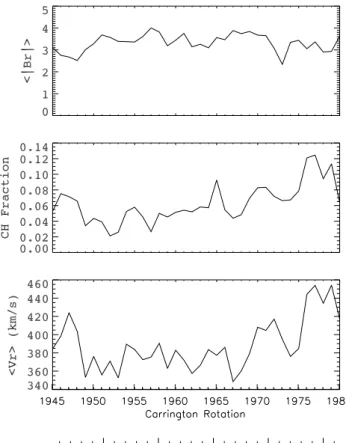
The evolution of the average properties of the parameters shown in Figs. 2–4 are shown in Fig. 5. In the top panel, the average value of the absolute value of Br is shown. And, al-though it does not show any obvious trend with solar cycle, there is significant variation during the 36 Carrington rota-tions; from a minimum of 2.4 to a maximum of 4, a change of ∼67%. The middle panel shows the fractional area cov-ered by coronal holes, obtained by integrating over the solar surface, and accounting for the sin(latitude) decrease in
el-Fig. 5. Evolution of the average magnitude of Br at the photo-sphere, the fractional area covered by coronal holes, and the average radial speed at 30 RSfrom CR1945 to CR1980.
emental area with increasing distance away from the equa-tor. There is a trend to higher values from CR1952 onward, with the percentage of the solar surface covered by coronal holes rising from 2% to a maximum of 12.5%. Similarly, in the bottom panel, the average value of the computed ra-dial velocity (itself dependent on the amount of open mag-netic field) shows a general increase during later Carring-ton rotations. The minimum average speed of ∼350 km s−1 occurred during CR1967 and the maximum average speed of ∼455 km s−1 occurred during CR1977 and CR1979. It is interesting to note that the time interval corresponding to the lowest average speed (CR1967: 3 September 2000– 30 September 2000) corresponds to the period when Ulysses measured its lowerest speeds (see Fig. 1).
5 Comparison of heliospheric structure at solar mini-mum and maximini-mum
Previously we have discussed the evolution of solar wind stream structure during the declining phase of the solar cy-cle (Riley et al., 2001a). Here, we focus on contrasting the difference between solar minimum and solar maximum con-ditions. The radial velocity is the primary driver of dynamic evolution, and as we have seen, the main change that occurs
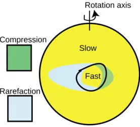
Fast Slow Fast Rotation axis Magnetic axis Fast Rotation axis Magnetic axis Slow Fast Compression Rarefaction View from opposite side of Sun
Fig. 6. Schematic of formation and orientation of streams at solar
minimum.
during the approach to solar maximum is the loss of a simple band of slow solar wind organized about the heliomagnetic equator, with high-speed wind bounding it on either side at higher latitudes. Near solar maximum, the flow conditions can better be described by slow, and more variable wind es-sentially everywhere, with pockets of high-speed flow. This fast wind is localized both in latitude and longitude.
Figure 6 is an extension of a schematic presented by Gosling et al. (1993) and illustrates how compression regions and rarefaction regions are generated during the declining phase of the solar cycle. Consider the simple “declining-phase” picture that we have alluded to several times of a band of slow solar wind about the heliomagnetic equator, which is tilted by some amount relative to the rotation axis. A par-cel of plasma launched from the northern edge of the slow flow band will eventually be caught by faster plasma to the east (left) of it, as the Sun rotates underneath and replaces the plasma source under that particular radial trace. The net effect is that, far from the Sun, a compression region builds, up organized about this region. When mapped back to the solar surface, the compression region would be located as shown in Fig. 6 (top). On the other hand, in the Southern Hemisphere, a similar argument leads to the formation of a
Fast
Rotation axis
Compression
Rarefaction
Slow
Fig. 7. Schematic of formation and orientation of streams at solar
maximum.
rarefaction region, as fast flow now outruns slower flow to the east. Finally, if we look at the opposite side of the Sun, the processes are reversed with a rarefaction region being set up in the Northern Hemisphere and a compression region in the Southern Hemisphere. We can extend the argument to account for more complex shapes of the slow-flow band. In particular, if it is warped or contains more than a single si-nusoidal variation with respect to heliographic latitude, the resulting patterns will be richer. Nevertheless, given the flow speed at some inner radial boundary, such as 30 RS, it is rel-atively straightforward to infer the resulting dynamical pat-tern.
At solar maximum, as we have seen, our boundary con-ditions have much less organization. The simplest case to consider is that of a single equatorial coronal hole giving rise to an isolated high-speed flow that is confined both in latitude and longitude. Such a configuration is summarized in Fig. 7. Applying the same arguments as before, we deduce that slow flow to the west of the equatorial coronal hole is caught by the fast wind, and compressed. East of the coronal hole, the slow flow is outrun by the fast wind generating a rarefaction region. The resulting structures are sideways “V” shapes.
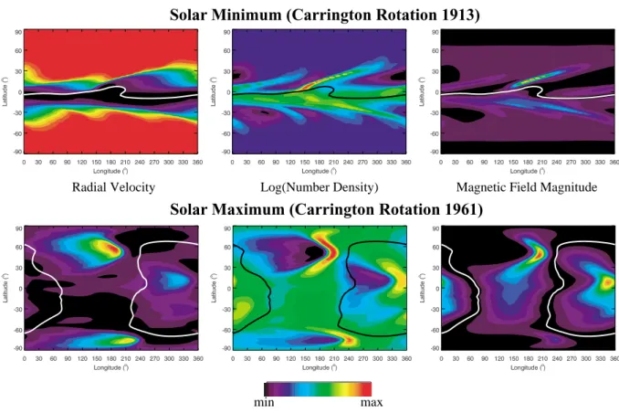
In Fig. 8 we compare simulation results from two extremes of the solar cycle. In the top row we summarize conditions typical of solar minimum (CR1913) at 4.35 AU (correspond-ing to the heliocentric distance of Ulysses at this time). The panels show solar wind speed, density (logarithmic), and magnetic field magnitude. Note how the slow wind is fined to a band about the equator, with the polar regions con-sisting entirely of fast wind. For purely radial flow then, compression regions arise where fast flow to the east (left) overtakes slower flow to the west (right). In contrast, rar-efaction regions occur when slower to the east (left) is out-run by faster flow to the west (right). Another way to look at this is to consider the Sun rotating underneath a spacecraft that is fixed in an inertial reference frame. The flow pattern rotates such that along a single radial trace plasma is succes-sively launched from points at earlier and earlier longitudes.
Solar Minimum (Carrington Rotation 1913)
Solar Maximum (Carrington Rotation 1961)
min max
Radial Velocity Log(Number Density) Magnetic Field Magnitude
Fig. 8. Comparison of solar wind structure at solar minimum (CR1913) and maximum (CR1961). The heliocentric distance of these slices
are 4.35 AU and 4.26 AU, respectively, corresponding to the location of the Ulysses spacecraft at these times. The columns show speed, density, and magnetic field magnitude. The solid white line in each panel denotes the location of the heliospheric current sheet.
A similar argument holds for rarefaction regions. The re-sultant pattern in the density (and magnetic field strength to a lesser extent) appears as a set of spurs off the slow-flow band.
In contrast, the bottom panels (at 4.26 AU) illustrate con-ditions at the peak of the solar cycle. Now the picture is one of isolated “beams” of solar wind punching through the slower, more prevalent wind. Where the beam catches slower wind ahead, compression regions form. At the trailing edges of the high-speed streams, rarefactions form. Their limited latitudinal and longitudinal extent, however, now gives rise to “V”-shaped interaction regions. Focusing on the lower-middle panel, we can identify 3 such profiles. Comparison with the radial velocity, shown in the lower-left panel, indi-cates that the sources are beams of high-speed wind plow-ing into slower wind ahead, generatplow-ing a pressure wave and compressing the plasma. Behind each “V”-compression is a larger expansion wave (or rarefaction region), trailing more than ∼180◦in longitude in some cases. Thus, although the high-speed streams are of limited latitudinal and longitudinal extent at the Sun, the rarefaction regions generated by them can span large regions of space.
Superimposed in each panel is the location of the helio-spheric current sheet (HCS). The evolution of the HCS over the course of a solar cycle has been discussed by Riley et al. (2002) and the detailed evolution of the interplanetary
mag-netic field, together with the HCS, during this time period will be the topic of a future study. Nevertheless, the compar-ison again serves to highlight the differences between condi-tions near solar minimum, where essentially all the “action” is confined to a band about the equator, and solar maximum, where the plasma and magnetic structures span essentially all latitudes.
6 Summary and discussion
In this report we have used 3-D MHD simulations to model the detailed evolution of the large-scale structure of the inner heliosphere during solar active conditions. In particular, we have used the simulations to describe the global evolution of the inner heliosphere during Ulysses’ second orbit descent to the southern polar regions, rapid latitude scan, and arrival into the northern polar regions. We found that the model reproduced the large-scale properties of the solar wind ob-served by Ulysses, although a detailed analysis of specific intervals is necessary to quantify how well the details of the stream structure are reproduced on the time scale of a single rotation. Preliminary analysis suggests that the model often produces relatively good matches, however, there are often intervals with poor correlation. Whether this is due to ap-proximations in the model, or due to the presence of CMEs
and other transient phenomena that are not included in the model remains to be seen.
There are several potentially significant sources of error in the model that can lead to inaccuracies in the solution. First and foremost, our resolution is limited to a few de-grees in latitude and longitude. While the coronal mod-els employ a non-uniform grid with spacing ranging from 0.018 RS to 3.1 RS, the heliospheric models use a uniform spacing of 15 RS. As such, our heliospheric solutions can-not resolve shocks, which, because of numerical diffusion, remain steepened waves. Second, our results represent aver-ages over a Carrington rotation. The photospheric magnetic field data used to drive the model was obtained over a pe-riod of0∼26 days from observations centered on the subso-lar point. Thus model results at longitudes significantly dif-ferent from Earth’s position must be carefully considered if significant evolution on the time scale of a solar rotation oc-curred. Ulysses observations, in particular, suffer from such an affect. Since it remains in essentially an inertial reference frame, it intercepts the Earth’s longitude once per year, stray-ing up to 180◦during the intervening times. At worst, then, the measurements made at Ulysses were produced by plasma launched from the opposite side of the Sun from the Earth, and thus, never directly visible from ground-based or near-Earth observatories. Third, we do not account for transient activity, and, in particular, coronal mass ejections. CMEs un-doubtedly perturb the ambient solar wind significantly, and we must therefore be careful when interpreting the observa-tions that none were obviously present. Fourth, our method of solution is not completely self-consistent. In particular, we use the expansion of the magnetic field to prescribe the variation in solar wind speed. This has been discussed in more detail by Riley et al. (2001a). And, while reasonable, and borne out empirically (Wang and Sheeley, 1990), it likely does not accurately mimic the more fundamental heating pro-cesses that are occurring in reality. Finally, in the absence of any reliable observations, our coronal model specifies uni-form temperature and density on the inner radial boundary.
The evolution of the solar magnetic field surrounding solar maximum is complex. At one end of the observational spec-trum, we have photospheric observations from which we can infer the radial component of the magnetic field. At the other end, we have in situ observations by spacecraft that provide detailed, although localized measurements of the magnetic field vector. One way to connect the two is through global MHD simulations. Riley et al. (2002) described the evolution of the HCS over the time scale of a solar cycle, including the time period modeled here. They found that during Carrington rotations 1960 and 1961, the typical “ballerina skirt” shape was replaced by a “conch shell”-like shape. In essence, rather than the HCS separating the northern and southern poles, it was localized in longitude, and both poles had the same polarity. This is supported by the photospheric field maps (Fig. 2), which show that during Carrington rotations 1960 and 1961 the polar fields were inward (blue) in both hemi-spheres. Moreover, when the Ulysses magnetic field polarity measurements were superimposed onto the global HCS
pat-tern, the phase of the polarity changes matched well. Without the simulations, the Ulysses observations might have been interpreted as a dipole-like field, as would have been seen during the late-declining phase of the solar cycle. It is also worth noting that this period does not coincide with the in-ferred magnetic field reversal, which occurred some 10 Car-rington rotations later.
The simulation results described in this study are available online at http://sun.saic.com. In addition to the parameters discussed here, we also provide some basic plotting tools to view all plasma and magnetic field parameters. Simulation data are also available, including simple routines to import the data into IDL. A movie showing the evolution of several of the key parameters discussed here can also be downloaded and played on an AVI or Quicktime compatible media player. We plan to expand this database in both directions, covering both the early Ulysses mission, as well as the most recent Carrington rotations. Ultimately, we hope that these simu-lations will develop into an operational tool, capable of pre-dicting ambient solar wind conditions at Earth (and beyond) with up to 4 days advanced warning.
Acknowledgements. We gratefully acknowledge the support of the National Aeronautics and Space Administration (Sun-Earth Con-nections Guest Investigator Program, Sun-Earth ConCon-nections The-ory Program, and Supporting Research and Technology Program) in undertaking this study. We also thank National Science Founda-tion at the San Diego Supercomputer Center for providing compu-tational support.
Topical Editor R. Forsyth thanks A. Gonzalez-Esparza and G. Erdos for their help in evaluating this paper.
References
Axford, W. I.: Interaction of the solar wind with the interstellar medium, in: Solar Wind, Space Science Reviews special issue on Outer Solar System Exploration-an Overview, 14, 582, (Eds) Sonett, C. P., Coleman, P. J., and Wilcox, J. M., 1973.
Balogh, A., Beek, T. J., Forsyth, R. J., Hedgecock, P. C., Mar-quedant, R. J., Smith, E. J., Southward, D. J., and Tsurutani, B. T.: The magnetic field investigation on the ulysses mission: Instrumentation and preliminary scientific results, Astron. Astro-phys. Supp. Series, 92, 221–236, 1992.
Bame, S. J., McComas, D. J., Barraclough, B. L., Phillips, J. L., Sofaly, K. J., Chavez, J. C., Goldstein, B. E., and Sakurai, R. K.: The ulysses solar wind plasma experiment, Astron. Astrophys. Supp. Series, 92, 237–265, 1992.
Fisk, L.: Motion of the footpoints of heliospheric magnetic field lines at the sun: Implications for recurrent energetic particle events at high heliographic latitudes, J. Geophys. Res., 101, 15 547–15 554, 1996.
Gonzalez-Esparza, J. and Smith, E.: Three-dimensional nature of interaction regions: Pioneer, voyager, and ulysses solar cycle variations from 1 to 5 AU, J. Geophys. Res., 102, 9781–9792, 1997.
Gosling, J. T., Bame, S. J., McComas, D. J., Phillips, J. L., Pizzo, V. J., Goldstein, B. E., and Neugebauer, M.: Lat-itudinal varia-tion of solar wind corotating stream interacvaria-tion regions: Ulysses, Geophys. Res. Lett., 20, 2789–2792, 1993.
Gosling, J. T., Feldman, W. C., McComas, D. J., Phillips, J. L., Pizzo, V. J., and Forsyth, R. J.: Ulysses observations of opposed tilts of solar wind corotating interaction regions in the northern and southern solar hemispheres, Geophys. Res. Lett., 22, 3333, 1995.
Gosling, J. T., Bame, S. J., Feldman, W. C., McComas, D. J., Riley, P., Goldstein, B. E., and Neugebauer, M.: The northern edge of the band of solar wind variability: Ulysses at – 4.5 AU, Geophys. Res. Lett., 24, 309, 1997.
Levine, R. J., Altschuler, M. D., and Harvey, J. W.: Solar sources of the interplanetary magnetic field and solar wind, J. Geophys. Res., 82, 1061–1065, 1977.
Linker, J. A., Miki´c, Z., Bisecker, D. A., Forsyth, R. J., Gibson, S. E., Lazarus, A. J., Lecinski, A., Riley, P., Szabo, A., and Thompson, B. J.: Magnetohydrodynamic modeling of the solar corona during whole sun month, J. Geophys. Res., 104, 9809– 9830, 1999.
McComas, D. J.: The three dimensional structure of the solar wind over the solar cycle, in Solar Wind 10, (Ed) Velli, M., AIP, Pisa, Italy, 2002.
McComas, D. J., Bame, S. J., Barraclough, B. L., Feldman, W. C., Funsten, H. O., Gosling, J. T., Riley, P., Skoug, R., Balogh, A., Forsyth, R. J., Goldstein, B. E., and Neugebauer, M.: Ulysses return to the slow solar wind, Geophys. Res. Lett., 25, 1–1, 1998. McComas, D. J., Gosling, J. T., and Skoug, R. M.: Ulysses observa-tions of the irregularly structured mid-latitude solar wind during the approach to solar maximum, Geophys. Res. Lett., 27, 2437– 2440, 2000.
McComas, D. J., Elliott, H. A., Gosling, J. T., Reisenfeld, D. B., Skoug, R., Goldstein, B. E., Neugebauer, M., and Balogh, A.: Ulysses second fast-latitude scan: Complexity near solar maxi-mum and the reformation of polar coronal holes, Geophys. Res. Lett., 29, 10.1029/2001GL014 164, 2002a.
McComas, D. J., Elliott, H. A., and von Steiger, R.: Solar wind from high latitude coronal holes at solar maximum, Geophys. Res. Lett., 29, 10.1029/2001GL013 940, 2002b.
Miki´c, Z., Linker, J. A., Schnack, D. D., Lionello, R., and Tarditi, A.: Magnetohydrodynamic modeling of the globalsolar corona,
Physics of Plasmas, 6, 2217–2224, 1999.
Pizzo, V. J.: Interplanetary shocks on the large scale: A retro-spective on the last decades theoretical efforts, in: Colli-sionless Shocks in the Heliosphere: Reviews of Current Research, Geo-phys. Monogr. Ser., 35, 51–68, 1985.
Pizzo, V. J.: The evolution of corotating stream fronts near the eclip-tic plane in the inner solar system. ii – three-dimensional tilted-dipole fronts, J. Geophys. Res., 96, 5405–5420, 1991.
Pizzo, V. J.: Global, quasi-steady dynamics of the distant solar wind 1: Origin of north-south flows in the outer heliosphere, J. Geo-phys. Res., 99, 4173–4183, 1994.
Pizzo, V. J. and Gosling, J. T.: 3-d simulation of high-latitude inter-action regions: Comparison with ulysses results, Geophys. Rese. Lett., 21, 2063–2066, 1994.
Riley, P., Gosling, J. T., Weiss, L. A., and Pizzo, V. J.: The tilts of corotating interaction regions at midheliographic latitudes, J. Geophys. Res., 101, 24 349–24 358, 1996.
Riley, P., Linker, J. A., and Miki´c, Z.: An empirically-driven global mhd model of the corona and inner heliosphere., J. Geophys. Res., 106, 15 889–15 902, 2001a.
Riley, P., Linker, J. A., Miki´c, Z., and Lionello, R.: Mhd model-ing of the solar corona and inner heliosphere: Comparison with observations, in Space Weather, Geophysical Monograph Series, 125, pp. 159–167, American Geophysical Union, Washington, D.C., 2001b.
Riley, P., Linker, J. A., and Miki´c, Z.: Modeling the heliospheric current sheet: Solar-cycle variations, J. Geophys. Res., 107, 2002.
Sarabhai, V.: Some consequences of nonuniformity of solar wind velocity, J. Geophys. Res., 68, 1555, 1963.
Smith, E. J. and Wolfe, J. H.: Observations of interaction regions and corotating shocks between one and five au: Pioneers 10 and 11, Geophys. Res. Lett., 3, 137–140, 1976.
Wang, Y. M. and Sheeley, N. R., J.: Solar wind speed and coronal flux-tube expansion, Astrophys. J., 355, 726–732, 1990. Wang, Y. M. and Sheeley, N. R. J.: The high-latitude solar wind