Eddy shedding from non-axisymmetric, divergent anticyclones with application to the Asian Monsoon anticyclone

Eddy Shedding from Non-axisymmetric, Divergent

Anticyclones with Application to the Asian

Monsoon Anticyclone

by

Chia-hui Juno Hsu

M.Sc. in Meteorology, National Taiwan University (1991)

B.Sc. in Physics, National Taiwan Normal University (1988)

Submitted to the Department of Earth, Atmospheric and Planetary

Sciences

in partial fulfillment of the requirements for the degree of

Doctor of Philosophy in Meteorology

at the

MASSACHUSETTS INSTITUTE OF TECHNOLOGY

@

Massachusetts

Setember 1998

L

cucuQ

\

cc4q

Institute of Technology 199

All rights reserved.

A u th or ...

Department of Earth, Atmospheric and Planetary Sciences

September 30, 1998

C ertified by ...

...

R. Alan Plumb

Professor in Atmospheric Sciences

Thesis Supervisor

Accepted by ...

:...

Ronald G. Prinn

Department Head

Eddy Shedding from Non-axisymmetric, Divergent

Anticyclones with Application to the Asian Monsoon

Anticyclone

by

Chia-hui Juno Hsu

Submitted to the Department of Earth, Atmospheric and Planetary Sciences on September 30, 1998, in partial fulfillment of the

requirements for the degree of Doctor of Philosophy in Meteorology

Abstract

The Asian summer Monsoon circulation is driven by differential thermal heating, primarily associated with the localized latent heat release from enhanced precipitation over the India sub-continent. Although this heating is of limited zonal extent, it drives a time-averaged, upper level anticylone which is of global extent, extending from the western edge of the bulge of Africa, to the east of the Asian continent. The current

theory (originally proposed by Gill (1980)) for explaining this zonally asymmetric component of the tropical circulation is unsatisfactory because it is based on the linear theory of damped equatorial waves while it is known that, at least for the upper level flow near the tropopause, the dynamics are strongly nonlinear. An alternative explanation, which is consistent with the nonlinear nature of the flows, involves the shedding of vortices from the directly forced monsoon anticyclone. The vortices, or eddies, are capable of drifting to the far field to establish a circulation which extends far beyond the local forcing.

This thesis provides a dynamical explanation for the generation of eddies near the center of a divergent anticyclone, which, through their westward drift are responsible for the establishment of the global scale of the Asian summer Monsoon. The thesis consists of two parts, one numerical and one observational. The numerical study systematically investigates localized thermally driven circulations by using a shallow water model. This part of the thesis is theoretical in nature, and seeks to under-stand how non-axisymmetric elements such as a beta effect, or an external uniform

flow, affects the dynamics of a divergent anticyclone for which, in the absence of

non-axisymmetric elements, there exists an analytical axisymmetric solution. Con-trol parameters which determine the dynamical regime of the flow are identified and explained. For the midlatitude beta plane experiment, the control parameter, pO, is the ratio between the free drift speed of an axisymmetric vortex on a beta plane, OL, and the strength of the forced localized divergent flow (ux) where L is the size of the axisymmetric circulation. For the uniform flow experiments, the control parameter

is the strength of the uniform flow, Urn, and the divergent flow, ux. Each control parameter measures the relative importance of two competing effects, one which tries to displace the anticyclone westward (for the midlatitude beta plane experiments), or downstream (for the uniform flow experiments) and one tries to keep the forced vortex anchored. For each series of experiments, a critical value which separates the different long-time flow behavior is found. When the circulation is below the critical value, the circulation is persistent and localized. When the control parameter is above the critical parameter, a material filament with low potential vorticity is drawn from the divergent center, rolls up due to shear instability and is soon shed away by detaching itself from the main vortex. In the time-mean vorticity budget, the transient eddies have the effect of dissipating the time-mean flow. The dissipation effect by transient eddies can be grossly parameterized as a linear damping term in the linear version of the model.

Another series of experiments, extending the midlatitude beta plane to the equa-torial beta plane, with an equator within the reach of the forced perturbation, is conducted in which equatorial waves can be generated. The shedding behavior be-gins when the value of the control parameter is of order unity in the midlatitude beta plane experiments, and continues to exist for values of order 10 in the equatorial beta plane experiments. When the control parameter takes on values of order 100 and larger, the shedding behavior disappears and is replaced by linear wave solutions. In these experiments, another non-dimensional parameter (q), which measures the non-dimensional distance from the thermal forcing center to the equator, is found to affect the stability characteristics of the forced vortex. This series of experiments also allows equatorial waves to co-exist with the nonlinear vortex and to be excited by the broad thermal cooling, whose magnitude and location are determined by the internal dynamics of the nonlinear forced vortex. This linear part of the response is similar to the solution predicted by Gill (1980), but is of opposite sign, since it is the response to the resulting broad thermal cooling part of the thermal forcing, and not the small localized imposed thermal heating as Gill would have it.

In the second part of the thesis, the theory is confirmed by discovering eddy shedding from the analysis of observational data. The potential vorticity on the isentropic surfaces are analyzed from 17 isobaric level NCEP-reanalysis data over the region of the Asian summer Monsoon. Two episodes of eddy shedding are found in July of 1990. The shedding events in the potential vorticity field are observed at the levels of isentropic surfaces from 360K to 380K. The induced geopotential perturbation penetrates deeper to 400 mb. The technique of Contour Advection with Surgery, a technique that allows to discriminate between adiabatic and diabatic effects, is used to recapture the shedding events, and confirm that the eddy shedding is indeed due to the essentially inviscid process identified in the idealized shallow water model.

Thesis Supervisor: R. Alan Plumb Title: Professor in Atmospheric Sciences

Notice

Doctoral Dissertation Defense of Thesis entitled:

Eddy Shedding from Non-axisymmetric, Divergent Anticyclones

with Application to the Asian Monsoon Anticyclone

by:

C. Juno Hsu

N6wJ7a,

wIAr

is

rlmt

souvo A&t ,' .5deD/v6- VaRTEX~(

TUNh

Prof.IJ R Fler _Glen

~U

Date:

Friday, August 07, 1998

Time:

2:00 PM

Place:

54-915, MIT

Thesis Committee:

Prof. Glenn R. Flieri

Dr. Isaac M. Held (GFDUPrinceton University)

Prof. Reginald E. Newell

Prof. R. Alan Plumb, Advisor

A copy of the thesis can be obtained at 54-1710.

Acknowledgments

On the day I started to write this acknowledgment, it was only three days from the date that I arrived at MIT, from the opposite side of the earth, six years ago. Six years would not be considered short for accomplishing most events in one's life time, probably a bit too long for a Ph.D. degree. During this period, there are many people involved in the final product presented in this thesis. There is an expression which I learned from a Chinese class in high school, "we can not thank all the people

by mentioning them one by one since there are so many; alternatively, we can only

express our gratefulness to the heavens". I am sure that there are more people than

I can remember who have helped me to go through different stages of my study at

MIT. I will always be thankful and can only hope to return the favors by helping others when I am given the opportunity.

I am indebted to my advisor, Prof. R. Alan Plumb. He let me struggle at my

own pace and yet gave me guidance when I needed it. Most of all, I felt particularly fortunate to have him as my advisor because his gentle character spares any possible agony from dealing with authority. I am grateful to Prof. Glenn R. Flierl who advised me closely and patiently during the semester of my thesis proposal. My knowledge about geophysical fluid dynamics is mostly acquired from him.

Prof. Reginald E. Newell served on my general exam and thesis committee. I would like to thank his participation and good intention. The generosity of Dr. Isaac M. Held of Princeton/GFDL for serving on my thesis committee is greatly appreciated. Dr. Held directed me to look for eddy shedding in the real atmosphere, which turned out to be invaluable for this study.

I would like to thank Frangois Primeau for proof-reading my thesis several times.

This thesis would not be readable if the prepositions, "in", "on"l, "for",etc., did not fall into the right places.

I would like to acknowledge my colleagues and officemates in meteorology for

scientific discussions and friendship over the years. They are Moto Nakamura, Dan Davidoff, Nili Harnik, Xinyu Zheng and Adams Sobel. James Risby is greatly thanked

for proof-reading my term papers, my general-exam paper and my thesis proposal. Jane McNabb will be missed not just for her administrative support, but mostly for her great spirit. Tracy Stanelun also provided a very friendly administrative environment when she worked at MIT. William Heres and Linda Meinke are thanked for their technical support.

Finally, I would like to thank Chen-An for his great spirit, care and encouragement over the past 6 years. Frangois was a good companion during the last stage of my study. I would like to dedicate this thesis to my parents and to my late brother, Chia-lu Hsu (1966-1997). I hope that by having completed this study, I can at least bring some comfort to my parents whose life have not been easy because of their kids.

Contents

1 Introduction

20

1.1 The chronicle of the thesis foretold . . . . 20

1.2 Synopsis of chapters ... ... ... 25

2 Background

26

2.2 Some fundamental properties of the tropical circulations . . . . 26

2.3 Gross observational features of the tropical large scale circulations . . 27

2.4 Current work related to large scale tropical circulations . . . . 33

2.4.1 Nonlinear inviscid theory for zonally-symmetric circulations: 33 2.4.2 Nonlinear inviscid theory for non-axisymmetric circulations: 34 2.4.3 Linear viscous theory for zonally-asymmetric circulations: . . . 36

2.5 The motivation of the thesis . . . . 38

3

Axisymmetric model

40

3.1

Introduction . . . .

40

3.2 Analytical solutions . . . . 41

3.3 1-D time-dependent simulation and linear instability analysis . . . . . 45

3.4 2-D time-dependent model . . . . 49

3.5 Summary of the chapter . . . . 55

4

Non-axisymmetric Model (1)

56

4.2

4.3

Scale analysis . . . . External uniform flow experiments . . . .

4.3.1 The model . . . .

4.3.2 The non-dimensional vorticity equation for the

experiments . . . .

4.3.3 Results and discussion . . . .

4.3.4 Sensitivity experiments . . . .

4.4 Mid-latitude

3

4.4.1 The model . . . .

4.4.2 The non-dimensional vorticity equation for

4.4.3 Results and discussions . . . .

4.4.4 Free vortex experiments . . . .

4.4.5 Role of transients . . . .

4.4.6 Sensitivity experiments . . . .

4.5 Summary of the chapter . . . .

5 Non-axisymmetric Model (2)

Equatorial 3-plane

5.1 Introduction . . . .

5.2 Equatorial beta plane experiments . . . .

5.2.1 The runs . . . .

5.2.2 Results and discussion . . . .

5.2.3 Summary for all the

3

5.3 Summary of the chapter . . . .

6 Observational Study

6.1 Introduction . . . .

6.2 The data and the technique of CAS . . . .

6.3 The results . . . .

6.4 Summary of the Chapter . . . .

uniform flow . . . . . . . . . . 70 -plane experiments 71 . . . . 72

. . . .

77

. . . .

99

101

7 Conclusions and future work

118

7.1 Conclusions . . . . 118

7.1.1 Results from numerical simulations . . . . 118

7.1.2 Results from observational study . . . . 120

7.1.3 Discussion and suggestions for future work . . . . 120

A Scale Analysis

122

A.0.5 The mass equation . . . . 123

List of Figures

1-1 The monthly mean surface precipitation rate for July of 1990 from

NCEP/NCAR Reanalysis. The contour interval is 4 x 10- kg m-2 s-1.

Only values greater than 1 x 10- kg m~2 s-' are contoured. .... 21

1-2 The monthly mean absolute vorticity scaled by the local planetary

vorticity at 200 mb for July of 1990. The contour interval is 0.1. Values

greater than unity (cyclonic shear) are not contoured. . . . . 22

1-3 The streamfunction at 200 mb for July 1990 plotted with a contour

interval of 5 x 106 m2s-1 . . . . 23

2-1 The monthly mean surface precipitation rate for January of 1990 from

NCEP/NCAR Reanalysis. The contour interval is 4 x 10-5kg m-2s-1 .

Only values greater than 1 x 10-' kg m- 2_s- 1 _{are contoured. . . . . . 28}

2-2 The zonal mean zonal wind and angular momentum distributions for July 1990. The contour interval for the zonal wind is 5 m s-1. The

contour interval for the angular momentum is 109m2 s--1. . . . . 29

2-3 The zonal mean wind field on the meridional plane for July 1990. The

dotted lines indicate the zonal mean vertical velocity in units of Pas-cal/sec. The contour interval is 0.005 PasPas-cal/sec. The dashed lines in

colors indicate meridional velocity. The contour interval is 0.5 ms-1 3 0

2-4 The upper level wind field at 200 mb for January 1990 plotted with

arrows. The solid contours plot the magnitudes of the wind field with

2-5 The velocity potential at 200 mb for January 1990. The contour

inter-val is 2 x 106m2_{s-1. . . . .}

_{. .}

2-6 The upper level wind field at 200 mb for July 1990 plotted with arrows.

The solid contours plot the magnitudes of the wind with a contour

interval of 15 m s . . . . . .. 32

2-7 The velocity potential at 200 mb for July 1990. The contour interval

is 2 x 106 m 2 s-1.

. . . .

3-1 Sketch of the imposed forcing in the 1-D axisymmetric, f-plane shallow

water model. The forcing has a Gaussian shape with an e-folding scale

b*, and a maximum amplitude 4D* on top of the basic geopotential (D*. 42

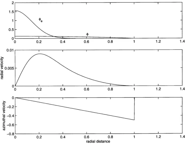
3-2 The steady state solution with r = 8.64, b = 0.2, and (e = 1.5625.

R=1 is the edge of the divergent circulation. . . . . 44

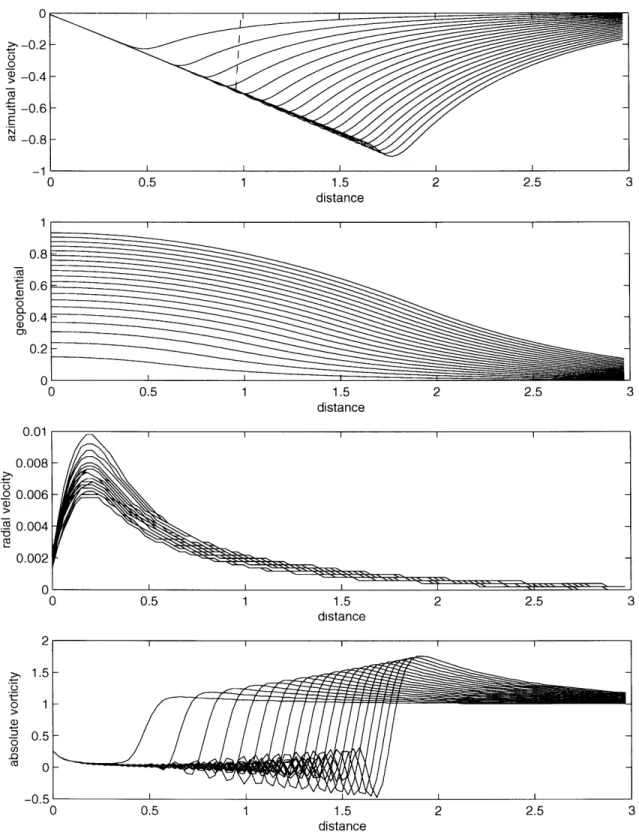
3-3 The 1-D time-dependent inviscid solution with T = 8.64, b = 0.2, and

'e

velocities, the geopotentials, the radial velocities and the absolute vor-ticities are displayed. Each panel contains 20 lines and each line rep-resents a snapshot of the model output. As time moves forward, the

lines move from the left to the right, or from the bottom to the top . 46

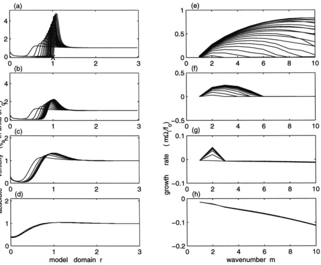
3-4 The Left panels (a)(b)(c)(d): the time evolution of the absolute

vor-ticity from the output of the 1-D time-dependent axisymmetric model

with the viscosity coefficent

v

10-from the top to the bottom. Each panel contains 20 lines and each line represent a snapshot from the model. As time moves forward, the lines moves from the left to the right. Notice the scales for (a)(b) are differ-ent from (c)(d). The right panels (e)(f)(g)(h):the growth rate scaled

by

fo

10. The corresponding basic flow for each panel is the left-hand side

panel. . . . . 48

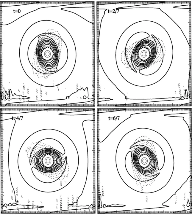
3-5 The second breaking cycle in the 2-D model with r = 8.64, b = 0.2,

<De = 1.5625, and v = 0. The contours are absolute vorticity scaled by

f

0

3-6 The shielded vortex collapses into a tripole with r = 8.64, b = 0.2, and

<be = 1.5625, and y = 4 x 10' in the 2-D model. The thick contours are

absolute vorticity scaled by

f,

and a minimum 0 in the center. The contour interval is 0.2. The solid thin lines are divergence with the contour interval which is 50 times

larger than the dashed thin lines representing the convergence. . . . . 52

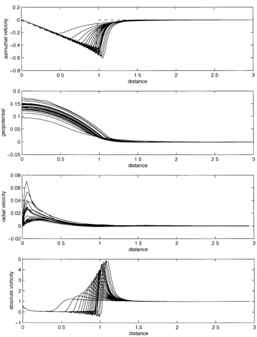
3-7 The 1-D time-dependent inviscid solution with T = 8.64, b = 0.2, and

<= 1.5625 but the Newtonian cooling term as the mass sink is turned

off. From the top panel to the bottom panel, the azimuthal velocities, the geopotentials, the radial velocities and the absolute vorticities are displayed. Each panel contains 20 lines and each line represents a snapshot of the model output. As time moves forward, the lines move from the left to the right, or from the bottom to the top. Compare

with Figure 3-3 . . . . 54

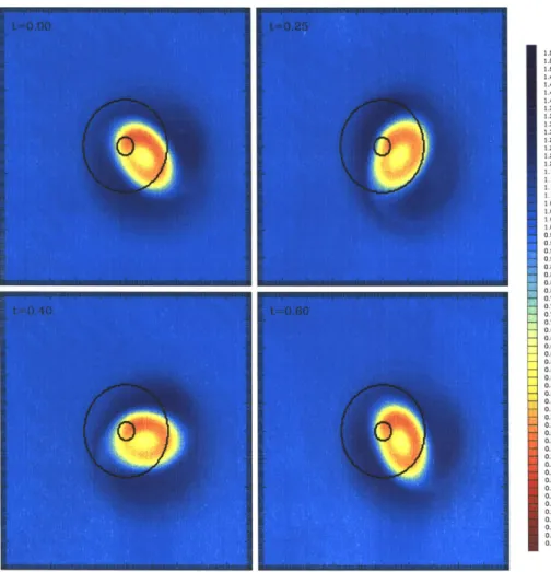
4-1 The phases of one wobbling cycle (t = 1) at t = 0, t = 0.25, t = 0.4, and

t = 0.6 for pmr = 0.55. The color contours are the absolute vorticity

with an interval of 0.025f0. The blue color indicates high absolute

vorticity and the red color indicates low absolute vorticity. The inner black circle marks the size of the imposed axisymmetric mass source and the outer circle marks the limit of the corresponding axisymmetric

4-2 The phases of one shedding cycle (t = 1) at t = 0.25, t = 0.5, t = 0.75 and t = 1.0 for pm = 1.93. The color contours are the absolute vorticity

with an interval of 0.025f0. The blue color indicates high absolute

vorticity and the red color indicates low absolute vorticity. The inner black circle marks the size of the imposed axisymmetric mass source and the outer circle marks the limit of the corresponding axisymmetric

divergent circulation if there were no uniform flow imposed. . . . . . 65

4-3 The time-mean absolute vorticity and wind field for pm = 0, Pm =

0.55, pm = 1.38, and ym = 2.48. The contours indicated the absolute

vorticity with the interval 0.1fo. The value at 0.5

f

with a thick contour. The center of the imposed forcing is marked by a cross, "X". The magnitudes of the wind should be multiplied by 1/50

to be scaled by the speed of the gravity waves. . . . . 66

4-4 The time-mean absolute vorticity and the divergence fields for pm =

0.27, pm = 0.55, pm = 1.10, pm = 1.38, pm = 1.93, and pm = 2.43.

The thick contours indicate absolute vorticity with a contour

inter-val 0.25

fo.

dashed contours indicate convergence. The former has a contour

inter-val 50 times larger than the latter. . . . . 68

4-5 The normalized-by-area divergence of transient vorticity flux (v'(') over

an area enclosed by a constant time-mean absolute vorticity at 0.5

(dashed-dot line), 0.6(dashed line), and 0.75 (solid lines). The

ab-scissa is the the control parameter pm and the ordinate is the vorticity

transport in dimensional unit s-. The nondimensional value can be

4-6 The phases of a shedding cycle (t = 1) at t = 0, t = 0.25, t = 0.5 and

t = 0.75 for p = 4.32. The color contours indicate absolute vorticity

with a contour interval 0.025

fo.

with a contour of 10 m2_s 2_{. The vectors are wind fields. The former}

should be multiplied by a factor of 1/2500, and the latter should be

multiplied by a factor of 1/50 to obtain the non-dimensional values. . 74

4-7 The phases of a wobbling cycle (t = 1) at t = 0.2, t = 0.4, t = 0.6 and

t = 0.8 for p = 0.43. . . . . 75

4-8 Time-mean absolute vorticity and the divergence fields for p = 0.09,

po = 0.43, po = 0.65, po = 0.86, p = 2.16, and pp = 4.32. The

thick contours indicate absolute vorticity with a contour interval 0.25

f.

contours indicate convergence. The former has a contour interval 50

times larger than the latter. . . . . 76

4-9 Trajectories of the free vortex for each

#

and from top to bottom for EXPI. The initial positions start at the origin and are plotted every -T denoted by circles for a period T

(De-1/2 b- 1

fo-

4-10 The westward and southward drifting speeds of the tripole on the corresponding beta plane of the forced experiments in a nonlinear model(EXP1) and a linear (EXP2) model. Results from EXPI are plotted in solid lines in which the smaller value is the southward speed. Results from EXP2 are plotted in dashed-dot lines where the southward

speeds are all nearly zero. The dashed line denotes 3L2 The abscissa

is the dimensional beta value which can be multiplied by 5 x 10" to obtain the non-dimensional value. The ordinate is the drifting speed

in ms- 1 which can be multiply by a factor of 1/50 to be scaled by the

4-11 The time mean distributions for po = 4.32. The top panel plots the

absolute vorticity with a contour interval of 0.1f0, and 0.5f,

empha-sized by a thick line. The lower panel plots the geopotential with an

interval of 20 m2s-2 which can be scaled by dividing a factor of 2500

m2 -2, the basic geopotential. The wind field can be multiplied by a

factor of 1/50 to obtain its non-dimensional version. . . . . 82

4-12 The vorticity balances for po = 4.32 and a calculated linear damping

term. (a) the time-mean advection term (b) the transient term (c) the planetary advection term (d) the vortex generation term (e) the diffusivity term (f) the time tendency term (g) the residual term from the summation of (a)-(e). (h) the linear damping term. The contour interval, 2 x 10-1 3_{s-2, is the same for each panel. A factor of 4 x 10"}

can be multiplied to obtain the non-dimensional value for Eq. 4.4.2 83

4-13 The steady state for linear run with p = 4.32. The contour plots are

the same as the nonlinear counterpart in Figure 4-11. . . . . 85

4-14 The linear steady state with po = 4.32 and the inclusion of a linear

damping term in the model with the coefficient r/. Compare this figure

5-1 (a) A snapshot of the model output with ,p3 = 2.16 and q=0.25. (b) A

snapshot of the model output with [tp = 2.16 and q=0.52. The color

contours show the absolute vorticity in units of

f.

total wind field where the wind magnitude should be multiplied by a factor of 1/258 for the top panel and 1/167 for the bottom panel to obtain the non-dimensional value if scaled by the speed of the gravity waves. The solid lines show contours of geopotential with the contour

interval, 500 m2s-2, which can be scaled by the basic geopotential

with the value, 66795 m2_s-2 _{for the top panel, and 28000 m}2_s-2 _for

the bottom panel. The inner black circle indicates the size of the imposed mass source, b. The outer black circle indicates the limit of the divergent axisymmetric circulation if there were no beta effect included in the model. Only the central part of the computational

domain between grid points

j=38

indicated, the plotted domain for each figure onwards is the same as

in this figure. . . . . 92

5-2 A snapshot of the model output with po = 2.16 and q=0.0625

(mid-latitude beta plane experiment). The color contours show the absolute

vorticity in units of

fo.

the wind magnitude should be multiplied by a factor of 1/50 if scaled

by the speed of the gravity waves. The solid lines show contours of

geopotential with the contour interval, 20 m2s-2_{, which can be scaled}

by the basic geopotential with the value, 2500 m2s-2. The inner black

circle indicates the size of the imposed mass source, b. The outer black circle indicates the limit of the divergent axisymmetric circulation if

there were no beta effect included in the model. . . . . 93

5-3 The analytical solution of Gill (1980) plotted in surface pressure and

surface wind vectors for a maximum heating located 100 to the north

5-4 A snapshot of the model output with p3 = 0.86 and q=0.38. The

color contours show the absolute vorticity in units of

f,.

are the total wind field where wind magnitude should be multiplied

by a factor of 1/118 to obtain the non-dimensional value scaled by the

phase speed of the gravity waves. The solid lines show contours of

geopotential where the contour interval is 500 m2s-2 which should be

divided by 14000 if scaled by the basic geopotential, 4%. The inner black circle indicates the size of the imposed mass source. The outer black circle indicates the edge of the divergent axisymmetric circulation

if there were no beta effect included in the model. . . . . 95

5-5 A snapshot of the model output with po = 17.28 and q=0.5. The color

contours show the absolute vorticity in units of

f

0

total wind field where wind magnitude should be multiplied by a factor of 50 to obtain the non-dimensional value scaled by the phase speed of the gravity waves. The solid lines show contours of geopotential

where the contour interval is 20 m2_s-2 _{for the bottom which should}

be divided 2500 respectively if scaled by the basic geopotential, 1D. The inner black circle indicates the size of the imposed mass source. The outer black circle indicates the edge of the divergent axisymmetric

circulation if there were no beta effect included in the model. .... 97

5-6 A snapshot of the model output with p3 = 172.8 and q = 5.0 (a) at

an early stage (b) for the steady state. The background contours are

absolute vorticity in units of

f,

absolute vorticity contours, the geopotential is plotted with a contour

interval 5 m2s-2 _{for the top panel and 20 m}2_s-2 _{for the bottom panel.}

The contour of zero absolute vorticity is emphasized. The equator is denoted by "E" and the forcing center is denoted by "X". The plotted

5-7 A summary plot of parameters in the p,3 - q domain for all the beta

-effect experiments. The ordinate indicates the parameter, p,3, and the

abscissa indicates the parameter, q. . . . . 99

6-1 Time sequence of PV field at 370K (color shading) and the geopotential

height at 200 mb (line contours) over the Asian summer monsoon at successive 6 hour time integrals starting from 18Z July 10 of 1990. The

color contour interval is 0.05 PVU. The lines contour is 25 m. . . . . 106

6-2 Continuation of Figure 6-1 . . . . 107

6-3 Continuation of Figure 6-2 . . . . 108

6-4 Time sequence of PV field at 380K (color shading) and the geopotential

height at 150 mb (black contours) over the Asian summer monsoon at successive 18 hour time intervals from OOZ July 11 to 06Z July 13 of

1990. The color contour interval is 0.05 PVU. The line contour interval

is 25 m . . . . . 109

6-5 Time sequence of PV field at 360K (color shading) and the geopotential

height at 250 mb (black contours) over the Asian summer monsoon at successive 18 hour time intervals from OOZ July 11 to 06Z July 13 of

1990. The color contour interval is 0.05 PVU. The line contour interval

is 25 m . . . . . 110

6-6 Time sequence of PV field at 350K (color shading) and the geopotential

height at 300 mb (black contours) over the Asian summer monsoon at successive 6 hour time intervals from OOZ July 11 to 06Z July 13 of 1990. The color contour interval is 0.05 PVU. The line contour interval is 25

m . . . . .. 111

6-7 Time sequence of PV field at 370K (color shading) and the geopotential

height at 200 mb (black contours) over the Asian summer monsoon at successive 6 hour time intervals from OOZ July 19 to OOZ July 20 of 1990. The color contour interval is 0.05 PVU. The line contour interval is 25

6-8 Continuation of Figure 6-7 . . . . 113

6-9 PV evolution at 360K over the Asian summer monsoon from CAS

technique, plotted at 4 successive 18 hour intervals. The initial field is 0.5, 0.75 and 1.0 PVU potential vorticity contours on 360K at 18Z

July 10 1990. . . . .. 114

6-10 PV evolution at 370K over the Asian summer monsoon from CAS

technique, plotted at 4 successive 18 hour intervals. The initial field is 0.5, 0.75 and 1.0 PVU potential vorticity contours on 370K at 18Z

July 10 1990. . . . . 115

6-11 PV evolution at 380K over the Asian summer monsoon from CAS

technique, plotted at 4 successive 18 hour intervals. The initial field is 0.5, 0.75 and 1.0 PVU potential vorticity contours on 380K at 18Z

July 10 1990. . . . . 116

6-12 passive contour evolution at 350K over the Asian summer monsoon

from CAS technique, plotted at 4 successive 18 hour intervals. The initial field is the 270, 280 and 290 mb pressure contours on 350K at

List of Tables

4.1 Uniform flow experiments: 4)e = 1.5625, b = 0.2, r = 8.64, V

4.0 x 10-4, -y = 6.25, K = 0.055. . . . . 61

4.2 midlatitude 3 effect experiments: 4e = 1.5625, b = 0.2, T = 8.64,

V = 4.0 x 10-4, -y = 6.5, r, = 0.055. . . . . 72

5.1 Equatorial beta effect experiments: p =_ (Geb2)-1/4tr and q =

(Oeb

)1 /40.

The values for T, 1e, b, and

#

B.1 Values of parameters for Chapter 3, Chapter 4 and Exps. No. 4 and

No. 5 of Chapter 5. . . . . 126

B.2 Values of beta used for the midlatitude / plane experiments. . . . . . 126

B.3 Beta values used for the equatorial

#

B.4 Values of variables used for Exp. No. 1-3 of equatorial / plane

Chapter 1

Introduction

1.1

The chronicle of the thesis foretold

The zonally-averaged component of the tropical circulation has drawn most of the at-tention in meteorology over the centuries since Hadley (1735), (see Lorenz, 1967 and Chapter 7 in Lindzen, 1990 for a review). Only until recently has a widely-accepted theoretical explanation based on the framework of zonally-symmetric models been provided (Schneider 1977; Held and Hou 1980; Lindzen and Hou 1988; Plumb and

Hou 1992). However, the theory would not be adequate without considering the

zonally-asymmetric component especially because (1) the distribution of the thermal forcing is far from zonally-symmetric and (2) the zonally-asymmetric component of the circulation is not just a small deviation from the zonally-symmetric component. Fig. 1-1 shows the monthly mean precipitation rate at the surface in July, 1990, representing the column integrated latent heat release - a major component of the thermal forcing. As shown in Fig. 1-1, the distribution is rather localized over the Asian Summer Monsoon area which is centered near 25'N and 90'E and is distin-guished from the zonally-elongated band along the ITCZ at 100 N. Fig. 1-2 shows the monthly mean absolute vorticity at 200 mb, scaled by the local planetary vorticity, for July 1990. As seen from the figure, there is a patch of low absolute vorticity contoured by the value of 0.5 in the area of heavy precipitation over Asian summer monsoon while the absolute vorticity is no lower than 0.6 for most of the areas in the

surface precipitation rate for July 1990

Figure 1-1: The monthly mean surface precipitation rate for July of 1990 from

NCEP/NCAR Reanalysis. The contour interval is 4 x 10- kg m- 2

S-1. Only values

greater than 1 x 10- kg m- 2 _s-1 _{are contoured.}

same latitudinal belt. This indicates a strong zonally asymmetric circulation over the Asian summer monsoon. Also, the large local Rossby number (-0.5) for this area suggests the importance of nonlinearity for the zonally asymmetric flow. In addition, it dominates the zonal mean.

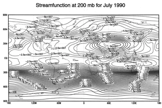
On the other hand, it is not the case that there is a lack of theory in meteorology to explain the zonally-asymmetric component of the circulation related to the Asian Summer Monsoon. There is a widely used model proposed by Gill (1980). However, as opposed to the nonlinear, inviscid zonally-symmetric model, this linear model requires a large mechanical damping term to obtain the right globle scale for the Asian summer monsoon. Fig. 1-3 shows a plot of the streamfunction at 200 mb for July 1990. The asymmetric circulation represented by the streamfunction is of global-scale. The last closed contour of the streamfucntion expands from 40'W to 160'E, covering over half of the global. While the linear parameterization term used in the linear model is justifiable for the low-level boundary flow (Neelin 1988; Lindzen and Nigam 1987), it is not obviously so for the upper level flow. For the upper level flow,

Monthly-mean absolute vorticity scaled by the local planetary vorticity at 200mb for July 1990

Figure 1-2: The monthly mean absolute vorticity scaled by the local planetary

vor-ticity at 200 mb for July of 1990. The contour interval is 0.1. Values greater than

unity (cyclonic shear) are not contoured.

the possible role of transient eddies in damping the global scale circulation is implied

from the vorticity budget calculation over the Asian Summer monsoon in a GCM

(Sardeshmukh and Held 1984). However, they give no explicit physical explanation

for the generation and subsequent propagation of eddies. Apart from the transient

eddies, cumulus friction is often considered as a dissipative agent on the large-scale

circulation (Holton and Colton 1972; Schneider and Lindzen 1977).

However, it

occurs only over small convective regions and therefore can not be responsible for the

large-scale damping. There is no a priori reason to assume that the time-mean upper

tropical flow is not inviscid (of course, this thesis in the end will provide a reason why

transient eddies can be the source of damping for the large scale circulation ).

Upon viewing the current available theories for the thermally-driven circulations,

one could see that there needs to be more work done to reconcile the current theories.

Schneider (1987) derived the zero absolute vorticity constraint (hereafter refer to as

ZAV and more details can be found in Section 2.4.2

)

for the steady non-axisymmetric

circulation to replace the constraint of the angular momentum conservation in the

axisymmetric model. This constraint is conceptually appealing since all the principles

used in the axisymmetric theory are still applicable to the non-axisymmetric case.

Physically, it states that the forced divergence decreases the absolute vorticity to zero

by squashing the vortex column, then the divergent flow further expands the material

with zero absolute vorticity outward by advection. In addition, the observational

study of Sardeshmukh and Hoskins (1985) near the tropics supports the idea of a

Streamfunction at 200 mb for July 1990

Figure 1-3: The streamfunction at 200 mb for July 1990 plotted with a contour

interval of 5 x 106 m

_s-

zero absolute vorticity ring being advected outward. In this thesis, we continue this

line of research and take the ZAV constraint idea as a basis for studying the

non-axisymmetric circulation.

The fundamental question of the thesis is as follows:

In a steady non-axisymmetric thermally-driven system, there must be solutions

which are nonlinear under a nearly inviscid assumption. What is the nature of the

solutions

?

Furthermore, how are these solutions related to the previously studied

2-D axisymmetric nonlinear inviscid solution and the linear non-axisymmetric viscous

solution ?

The early stage of the study focuses on building a system which can carry the

property of angular momentum conservation over to the ZAV solution along with

the requirement of using localized forcing. As a consequence, the simplest system,

a shallow water system on an f-plane, is chosen. A 1-D axisymmetric system is

used to realize the flow and its stability properties. The non-axisymmetric study is

started by breaking the axis-symmetry of f-plane solution by progressively adding asymmetric elements. The inclusion of asymmetric elements is kept simple. In one set of experiments, a uniform flow is imposed in a 2-D model with doubly periodic

boundary conditions. In another set of experiments, a beta effect is imposed in

the 2-D channel model. The aim is to keep the dynamics relatively easy to grasp. Initially the focus is on understanding the dynamics of the steady non-axisymmetric solutions and the extent to which the ZAV constraint can be satisfied. Subsequently, the attention shifts to a parameter regime beyond which the steady solution becomes unstable. In this regime, it is found that transient eddies are detached from the forced vortex and drift to the far field. Attention is drawn to this parameter regime because of the importance of transient eddies over the Asian Summer Monsoon emphasized

in a budget study by Sardeshmukh and Held (1984). At this stage, the following

question is studied:

Does the eddy shedding observed in the model have the effect of dissipating the

time-mean circulation ?

When such a role is confirmed, the conflicting theories are partly reconciled. The non-axisymmetric circulation with eddy-shedding is in the nonlinear regime though not in the ZAV regime. The transient eddies carry low PV to the far field and eventually establish a global scale circulation. The role of eddies as a dissipation agent seems to provide a physical reason for the use of large mechanical damping in linear models. With this in mind, we go back to examine the dynamics near the upper troposphere in the Asian Summer Monsoon. Based on the simple model studies, the absolute vorticity should be low over the intense divergent area in the upper troposphere, though not necessarily zero, and there should be eddies shed from the divergent area which propagate westward to build a global-scale circulation. If one forms a zonal average, the angular momentum should be almost conserved because of the sum over several local heating blobs. This leads to the following question:

Is there eddy-shedding taking place in the Asian Summer Monsoon region ?

1.2

Synopsis of chapters

Chapter 2 contains a review of the general circulation of the tropical and subtropical dynamics. It includes two parts. First, we construct an overall picture of the summer circulation based on the NCEP-reanalysis data for 1990. Second, existing theories to explain the different components of the circulations are reviewed. This is followed

by discussion on how well the theories can explain the observations and the

consis-tency among the theories. Chapter 3 contains the construction of an axisymmetric inviscid steady state solution as well as a time-dependent solution. However, these inviscid solutions are in general unstable to asymmetric perturbations. The inclusion of Laplacian diffusion is studied with a normal mode analysis and time dependent solution as a mean of obtaining a stable nearly axisymmetric solution with the least amount of viscosity. Chapter 4 consists of two parts. The first part discusses how a simple imposed uniform flow can destroy the axisymmetry and how it affect the flow's behavior. The second part discusses how a prescribed beta effect on a midlatitude

3

vor-tex drift experiments are included to shed some insight on the physics of the forced

experiments. Chapter 5 contains equatorial

#

within the reach of the forced perturbations. Chapter 6 presents the results from the

observational study of NCEP/NCAR reanalysis data. Chapter 7 has a summary of

Chapter 2

Background

2.1

Introduction

This chapter provides the background for the observational and theoretical aspects of the large-scale tropical circulations. The purpose is to motivate this thesis by reviewing certain inconsistencies in the current theories. Section 2.2 lists some ba-sic properties of the tropical circulations. Section 2.3 has a brief description of the zonally-averaged and zonally-asymmetric circulations from the observational data. Section 2.4 discusses some currently available theories for these circulations. Sec-tion 2.5 discusses how the inconsistencies among the current theories motivates this thesis and also provides the justification for the model that we use in this study.

2.2

Some fundamental properties of the tropical

circulations

Unlike the mid-latitude atmospheric dynamics which can be understood in the frame-work of the quasi-geostrophic system, there is no such simple theoretical frameframe-work to provide an overall understanding of the large-scale tropical circulations. A general discussion of large scale tropical circulation can be found in Paegle et. al. (1983) and Webster (1983). However, some basic properties are known to be manifestations of

the smaller rotational rate and the larger differential rotational rate of the earth, and of the moist atmosphere (Holton 1972). We list some of them to guide our choice of parameter for our study of the tropics:

e In contrast to the baroclinic environments present in midlatitudes, the

tropics has small temperature gradients. Tropical motion primarily gains its kinetic energy via the vertical redistribution of heat. In the thermo-dynamic equation, the leading balance is between the diabatic heating (cooling) and the adiabatic cooling (warming).

e For a synoptic scale system, the Rossby number is equal to or greater

than one. However, the linear planetary vorticity advection term is also large since beta has a maximum at the equator. For a similar system, the pressure variation is one order smaller than that in midlatitudes.

2.3

Gross observational features of the tropical large

scale circulations

In the tropics, the primary heating agent for the atmosphere is the large zonal array of individual cumulonimbus clouds in the Intertropical Convergence Zone (ITCZ), the South Pacific Convergence Zone (SPCZ) and mosoonal regions. The ITCZ lies to the north of the equator across the Pacific and Atlantic oceans and the SPCZ branches from the ITCZ across the southwestern tropical Pacific and ends south of the equator. These convergence zones migrate north-south with the warm sea surface temperature (see a more detailed description in Philander (1990)). Figure 2-1 shows the surface precipitation rate for January of 19901 to be compared with the precipitation rate in Figure 1-1 for July of 1990. As shown form the figures, the ITCZ and SPCZ can be identified from the zonally oriented line sources near 10'N in July and north and south of the equator in January. In addition, the asymmetry of the

'The year 1990 is considered to be a "typical" year here. The monthly mean figures are given for illustration purpose by assuming they are not too different from climatology.

surface precipitation rate for January 1990

Figure 2-1: The monthly mean surface precipitation rate for January of 1990 from

NCEP/NCAR Reanalysis. The contour interval is 4 x 10-5kg m-2_s-1_{. Only values}

greater than 1 x

10-

heating distribution is largely enhanced over the three continents: South America and Africa and the maritime continent of Indonesia and Malaysia. In January, the heating maximum straddles the maritime continent at 1200 near the equator. In July, the heating maximum moves northward to 25*N over Asia, separating itself from the line heating sources over the oceans and appearing more localized in the Asian subtropical region. There are three major thermally-driven circulations associated with the heating distributions. The Hadley circulation consists of the north-south overturning circulation out of the ITCZ and SPCZ. Its zonally-averaged features are illustrated in the zonal wind and angular momentum distributions in Figure 2-2, and the wind field on the meridional plane is shown in Figure 3. As shown from Figure 2-2, two subtropical westerly jets are located at 30*S in the winter hemisphere and at 45 *N in the summer hemisphere. In addition, there are weak easterlies throughout the tropics. A strong meridional overturning cell with air rising from the summer side of the equator with a maximum strength at ~ 80 N and air sinking in the winter

Zonal mean zonal wind and angular momentum distributions for July 1990

Figure 2-2: The zonal mean zonal wind and angular momentum distributions for July

1990. The contour interval for the zonal wind is 5 m s-'. The contour interval for

the angular momentum is 109m2 S-1.

cell sinks poleward of the main cell.

The second major thermally-driven circulation is the Walker circulation - the

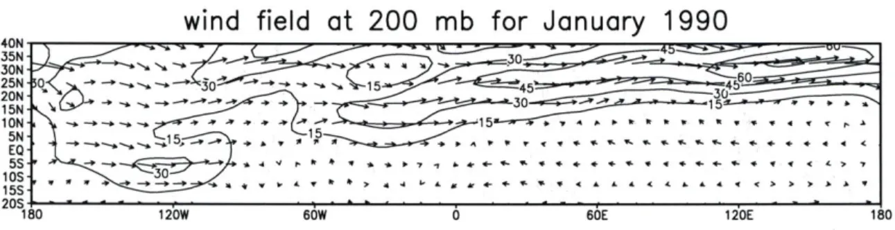
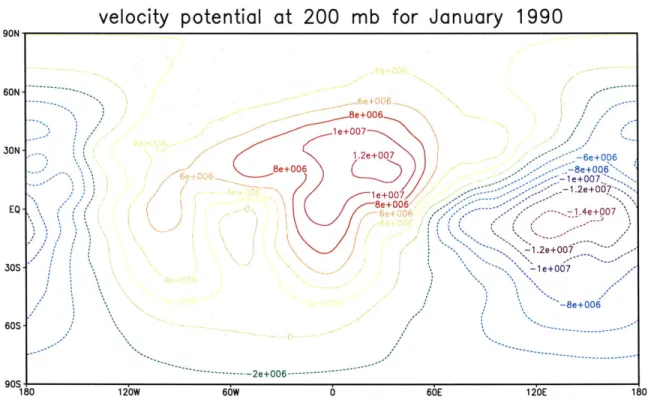
east-west overturning circulation out of ITCZ and SPCZ with a stronger strength in the winter. Figures 2-4 and 2-5 show the wind field and velocity potential at 200 mb for January of 1990. The upper branch of the Walker circulation can be constructed from Figure 2-4 and Figure 2-5 by following the strong westerlies along the equator from the divergent center over the maritime continent to the weak convergent center near the western coast of South America.

In July, the upper divergent center moves to the north in accordance with the movement of the maximum heating over the Asian continent. The more prominent

zonal mean meridional circulation for July 1990

Figure 2-3: The zonal mean wind field on the meridional plane for July 1990. The dotted lines indicate the zonal mean vertical velocity in units of Pascal/sec. The contour interval is 0.005 Pascal/sec. The dashed lines in colors indicate meridional velocity. The contour interval is 0.5 ms-1

wind field at 200 mb for January 1990

4UN 35N 30N 25N 20N 15N 1 ON 5N-EQ 5S- 155- 20S-180 120W 1 2OE

Figure 2-4: The upper level wind field at 200 mb for January 1990 plotted with arrows. The solid contours plot the magnitudes of the wind field with a contour interval of

15 ms--.

velocity potential at 200 mb for January 1990

Figure 2-5: The velocity potential at 200 is 2 x 106m2s-1.

0 60E 120E 180

mb for January 1990. The contour interval

circulation is the third thermally-driven circulation- the Asian Summer Monsoon.

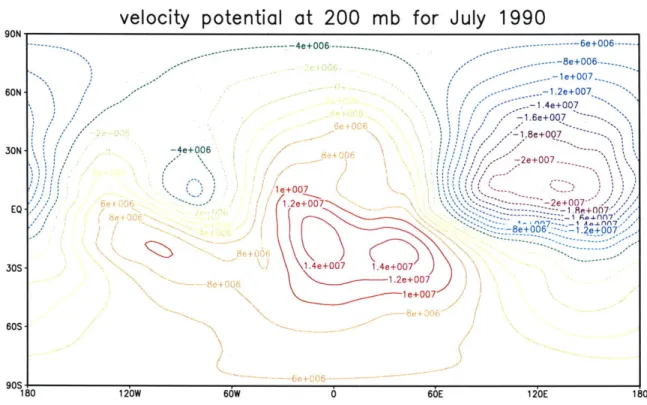
Figures 2-6 and 2-7 show the wind field and potential velocity distributions at 200 mb for July of 1990. As we discussed previously in Section 1.1, there is a global-scale anticyclonic circulation over the divergent center in the subtropics near 90'E where the divergent flow emanates and has a maximum strength as can be seen from the strong gradient of velocity potential in Figure 2-7. There are strong cross-equatorial flows in the southern branch of the circulation and the overturning cell seems to extend to the East Pacific Ocean as shown from the velocity potential distribution in Figure 2-7 as well as the wind distribution in Figure 2-6.

---

40N 35N 30N 25N 20N 1 5N iON- 5N- EQ- 5S- 15S-

20S-wind field at 200 mb for July 1990

0 120W 1 20E

Figure 2-6: The upper level wind field at 200 mb for July 1990 plotted with arrows. The solid contours plot the magnitudes of the wind with a contour interval of 15

ms 1.

velocity potential at 200 mb for July 1990

Ofl i -4e -4e+00 6 1e+007 1.2e+00 1.4e 006 14 06-- --6e+006 --- 8e+006---1e+007 --- 1.2e+007 1.4e+007 - , -1.6e+007 -1.8e+007 -2e+007 7 -- 2e+007 - 4-nn --- - -1.8e+00 8e+006- 1 2e+007 +007 1.4e+007 1.2e+007 1 e+007 1 20E

Figure 2-7: The velocity potential at 200 mb for July 1990. The contour interval is 2 x 106 m2 _s-'. -+ *!5a-+-

+*

~

~

~4----

2.4

Current work related to large scale tropical

circulations

2.4.1

Nonlinear inviscid theory for zonally-symmetric

circu-lations:

There has been a series of theoretical studies on zonally axisymmetric thermally driven circulations (Schneider 1977; Held and Hou 1980; Lindzen and Hou 1988;

Plumb and Hou 1992; Zhang 1997). A detailed historical review on the zonally

averaged circulations can be found in Lorenz (1967), and a detailed discussion on the dynamics can be found in Chapter 7 of Lindzen (1990). Here we briefly go over the calculation of the steady state solution based on Held and Hou's paper (1980). Based on the same principles, we derive in Chapter 3 a solution analogous to Held and Hou's for an f-plane shallow water model.

The assumption that the fluid is inviscid is the basic assumption for these axisym-metric theories. For a steady, inviscid symaxisym-metric flow, Schneider (1977) pointed out, from the extension of Hide's theorem (1969), that there should be no maximum of angular momentum anywhere except at the surface of regions with surface easterlies. This theorem selects either of the two possible steady solutions which are referred to as Thermal Equilibrium solution and Angular Momentum Conserving solution (Plumb and Hou (1992) has a detailed discussion on the selection of these solutions). For a stratified fluid on a sphere, the system can be thermally driven by relaxing back

to an imposed "convective - radiative" equilibrium state. The imposed thermal

equi-librium state itself is a solution provided its angular momentum distribution has no maximum in the interior of the fluid. When it does, a solution based on angular mo-mentum conservation replaces it. The vertically-averaged temperature is calculated

by assuming the zonal flow is balanced. The latitudinal extension of the angular

mo-mentum conserving solution is decided by requiring that there is "no heat loss within the circulation". Beyond the overturning circulation, the solution is connected to the thermal equilibrium solution by imposing continuity in the temperature field. At the

matching point, the zonal flow, however, is not continuous. If a parcel starts from rest and moves from 10*N all the way to 40*S, its zonal velocity would reach 231.6

ms-1 by angular momentum conservation.

If the imposed equilibrium temperature is symmetric about the equator, two equal

cells on both sides of the equator develop (Held and Hou 1980). If one moves the heating profile off the equator by a few degrees, one large cell extending to the winter hemisphere and another weak cell poleward of the main cell develop (Lindzen and Hou 1988). If the heating maximum is further moved into the region of the subtropic where the Coriolis parameter is finite, no meridional overturning circulation possible unless a certain critical thermal forcing amplitude is reached (Plumb and Hou 1992;

Zhang 1997).

2.4.2

Nonlinear inviscid theory for non-axisymmetric

circu-lations:

The constraint of angular momentum conservation is the basis on which symmetric flow solutions discussed above are derived. In a non-axisymmetric flow, angular mo-mentum is not conserved. However, the property of zero absolute vorticity (which is proportional to the derivative of angular momentum in symmetric flow) can be carried over the the non-axisymmetric flows. Schneider (1987) derived such an inte-gral constraint from the circulation equation. For the shallow water system (or for the 3 dimensional hydrostatic, primitive system, we consider the outflow layer in the tropics where the vertical velocity is small and the vortex twisting term is assumed to be small), the circulation tendency for the time-mean flow U, around any closed contour C is

dl+ V-jidA=- V-(U)dA+ F-d1, (2.1)

where A is the area enclosed by that contour, and the terms on the right describe the contributions of transient eddies and friction, respectively. In an inviscid steady state with no transient eddies, if we choose C to be a closed contour of absolute vorticity

(~ (=constant), the equation reduces to

af

V - dA = 0.

_(2.2)

Which implies two possibilities:

( = 0 or JV dA

= 0.

Sobel and Plumb (1998) have shown that this result holds true for inviscid flow even in the presence of transients, provided the area enclosed by the contour does not change with time. If the absolute vorticity contour is zero, there is no constraint on the divergence distribution in the region which is enclosed by the contour. If the absolute vorticity contour is not zero, the integrated divergence over the area enclosed by the contour has to be zero. In such a case, there would be an equal amount of mass source and sink within any enclosed contour of absolute vorticity with non-zero value. However, solving the analytical non-axisymmetric thermally driven circulations by using the above constraints is not easy. Schneider (1987) solved the problem by assuming the zonally asymmetric component is only a small perturbation to the zonally symmetric part.

The idea of zero absolute vorticity is not just a theoretically interesting way of replacing the angular momentum conservation solution for non-symmetric flow. Ob-servational studies show that the atmosphere does have regions of near zero absolute vorticity. Sardeshmukh and Hoskins (1985) calculated the vorticity budget over the east equatorial Pacific Ocean at 150mb, near the level of maximum outflow associated with organized deep convection in the tropics during the 1982-83 El Niio-Southern Oscillation event. They found state that the vorticity balance is nonlinear and nearly inviscid. Furthermore, they state that the idea of zero absolute vorticity- outward expansion of material circuits in regions of convective outflow leads to a rapid

spin-down of fluid column, a zero absolute circulation - is of crucial importance. In a

Asian Summer Monsoon in a GCM, Sardeshmukh and Held (1984) also find that the balance is essentially nonlinear and inviscid. In the real atmosphere, a steady state is hardly achieved. However, the concept of material of zero absolute vorticity expanding outward is useful for thinking about non-axisymmetric thermally-driven circulation forced by localized heating. Other works addressing the importance of nonlinearity for the upper tropcial circulation include Nobre (1983) and Hendon (1985).

2.4.3

Linear viscous theory for zonally-asymmetric

circula-tions:

The most prevalent theory regarding the asymmetric response of the tropical atmo-sphere is based on equatorial waves (Matsuno 1966). Gill (1980) used a linear shallow water model on an equatorial beta plane to study the atmospheric response to local-ized heating at the equator and off the equator. The solution he derives consists of forced stationary equatorial waves. This Kelvin wave, which consists of zonal flows trapped near the equator, is proposed to explain the Walker circulation. When the heating is moved further away from the equator, a forced Rossby wave dominates the response and it is proposed to explain the global-scale anticyclone over the Asian Summer Monsoon. However, to confine the circulations to a finite distance, a large linear dissipation is required in the model. Since the zonal scale of the circulation is proportional to the group velocity times the dissipation time scale, a dissipative time scale of 2.5 days is needed to confine the circulation to a realistic extent to explain the Walker circulation. Notice that for a zonally averaged linear model only the dissipation term can balance the Coriolis force in the zonal direction. Extensions to the linear model include the study of Lau and Lim (1982) where they study the time-dependent version of Gill's model (1980), Heckley and Gill (1984) who study the time-dependent analytical solution to a steady localized heating and Philip and Gill (1987) who re-derive the steady state solutions by adding a uniform zonal flow. More recently Zhang and Krishnamurti (1996) used more realistic forcing from the OLR distribution over the tropical belt to rederive Gill's analytical solution.