HAL Id: inria-00120408
https://hal.inria.fr/inria-00120408
Submitted on 14 Dec 2006
HAL is a multi-disciplinary open access
archive for the deposit and dissemination of
sci-entific research documents, whether they are
pub-lished or not. The documents may come from
teaching and research institutions in France or
abroad, or from public or private research centers.
L’archive ouverte pluridisciplinaire HAL, est
destinée au dépôt et à la diffusion de documents
scientifiques de niveau recherche, publiés ou non,
émanant des établissements d’enseignement et de
recherche français ou étrangers, des laboratoires
publics ou privés.
Handwritten Chinese character recognition: Effects of
shape normalization and feature extraction
Cheng-Lin Liu
To cite this version:
Cheng-Lin Liu. Handwritten Chinese character recognition: Effects of shape normalization and feature
extraction. Arabic and Chinese Handwriting Recognition (SACH06), Sep 2006, Maryland / USA,
United States. �inria-00120408�
Handwritten Chinese Character Recognition: Effects of Shape
Normalization and Feature Extraction
Cheng-Lin Liu
National Laboratory of Pattern Recognition (NLPR)
Institute of Automation, Chinese Academy of Sciences (CASIA)
PO Box 2728, Beijing 100080, P.R. China
E-mail: [email protected]
Abstract
The field of handwritten Chinese character recog-nition (HCCR) has seen significant advances in the last two decades, owing to the effectiveness of many techniques, especially those for character shape normalization and feature extraction. This paper reviews the major methods of normalization and feature extraction, and evaluates their perfor-mance experimentally. The normalization meth-ods include linear normalization, nonlinear normal-ization (NLN) based on line density equalnormal-ization, moment normalization (MN), bi-moment normaliza-tion (BMN), modified centroid-boundary alignment (MCBA), and their pseudo-two-dimensional (pseudo 2D) extensions. As to feature extraction, we fo-cus on some effective variations of direction features: chaincode feature, normalization-cooperated chain-code feature (NCCF), and gradient feature. We have compared the normalization methods previ-ously, but in this study, will compare them with better implementation of features. As results, the current methods perform superiorly on handprinted characters, but are insufficient for unconstrained handwriting.
1
Introduction
Since the first work of printed Chinese charac-ter recognition (PCCR) was published in 1966 [1], many research efforts have been contributed, to both printed and handwritten Chinese character recogni-tion (HCCR). Research on online HCCR was started as early as PCCR [2], whereas offline HCCR was started in late 1970s, and has attracted high atten-tion from the 1980s [3]. Since then, many effective methods have been proposed to solve this problem, and the recognition performance has advanced sig-nificantly [4, 5]. This paper is mainly concerned with
offline HCCR, but most methods of offline recogni-tion are applicable to online recognirecogni-tion as well [6].
The approaches of HCCR can be roughly grouped into two categories: feature matching (statistical classification) and structure analysis. Based on ture vector representation of character patterns, fea-ture matching approaches usually computed a sim-ple distance measure (correlation matching), say, Euclidean or city block distance, between the test pattern and class prototypes. Currently, sophisti-cated classification techniques [7, 8, 9], including parametric and non-parametric statistical classifiers, neural networks, support vector machines (SVMs), etc., can yield higher recognition accuracies. Nev-ertheless, the selection and extraction of features remains an important issue. Structure analysis is an inverse process of character generation: to ex-tract the constituent strokes and compute a struc-tural distance measure between the test pattern and class models. Due to its resembling of human cog-nition and the potential of absorbing large deforma-tion, this approach was pursued intensively in the 1980s and is still advancing [10]. However, due to the difficulty of stroke extraction and structural model building, it is not widely followed.
Statistical approaches have achieved great success in handprinted character recognition and are well commercialized due to some factors. First, feature extraction based on template matching and classi-fication based on vector computation are easy to implement and computationally efficient. Second, effective shape normalization and feature extraction techniques, which improve the separability of pat-terns of different classes in feature space, have been proposed. Third, current machine learning methods enable classifier training with large set of samples for better discriminating shapes of different classes. The methodology of Chinese character recogni-tion has been largely affected by some important techniques: blurring [11], directional pattern
match-ing [12, 13, 14], nonlinear normalization [15, 16], modified quadratic discriminant function (MQDF) [17], etc. These techniques and their variations or improved versions, are still widely followed and adopted in most recognition systems. Blurring is ac-tually a low-pass spatial filtering operation. It was proposed in the 1960s from the viewpoint of human vision, and is effective to blur the stroke displace-ment of characters of same class. Directional pat-tern matching, motivated from local receptive fields in vision, is the predecessor of current direction his-togram features. Nonlinear normalization, which regulates stroke positions as well as image size, sig-nificantly outperforms the conventional linear nor-malization (resizing only). The MQDF is a nonlin-ear classifier suitable for high-dimensional features and large number of classes. Its variations include the pseudo Bayes classifier [18], the modified Maha-lanobis distance [19], etc.
This paper reviews the major normalization and feature extraction methods and evaluate their per-formance in offline HCCR on large databases. The normalization methods include linear normaliza-tion (LN), nonlinear normalizanormaliza-tion (NLN) based on line density equalization [15, 16], moment nor-malization (MN) [20], bi-moment nornor-malization (BMN) [21], modified centroid-boundary alignment (MCBA) [22], as well as the pseudo-two-dimensional (pseudo 2D) extensions of them [23, 24]. These methods have been evaluated previously [24], but in this study, they will be evaluated with better im-plementation of features.
Though many features have been proposed for character recognition, we focus on the class of rection histogram features, including chaincode di-rection feature, normalization-cooperated chaincode feature (NCCF) [25], and gradient direction feature. These features have yielded superior performance due to the sensitivity to stroke-direction variance and the insensitivity to stroke-width variance. The gradient direction feature was not paid enough at-tention until the success of gradient vector decompo-sition [26], following a decompodecompo-sition scheme previ-ously proposed in online character recognition [27]. Alternatively, the direction of gradient was quan-tized into a number of angular regions [28]. By NCCF, the chaincode direction is taken from the original image instead of the normalized image, but the directional elements are displaced in normalized planes according to normalized coordinates. An im-proved version of NCCF maps chaincodes into con-tinuous line segments in normalized planes [29].
In the history, some extensions of direction fea-ture, like the peripheral direction contributivity
(PDC) [30] and the reciprocal feature field [31], have reported higher accuracy in HCCR when simple dis-tance metric was used. These features, with very high dimensionality (over 1,000), are actually highly redundant. As background features, they are sensi-tive to noise and connecting strokes. Extending the line element of direction feature to higher-order fea-ture detectors (e.g., [32, 33]) helps discriminate sim-ilar characters, but the dimensionality also increases rapidly. The Gabor filter, also motivated from vi-sion research, promises feature extraction in charac-ter recognition [34], but is computationally expen-sive compared to chaincode and gradient features, and at best, perform comparably with the gradient feature [35].
We evaluate the character shape normalization and direction feature extraction methods on two databases of handwritten characters, ETL9B (Elec-trotechnical Laboratory, Japan) and CASIA (Insti-tute of Automation, Chinese Academy of Sciences), with 3,036 classes and 3,755 classes, respectively. Two common classifiers, minimum distance classi-fier and modified quadratic discriminant function (MQDF), are used to evaluate the recognition ac-curacies.
The purpose of this study is twofold. First, the comparison of major normalization and feature ex-traction methods can provide guidelines for selecting methods in system development. Second, the results show to what degree of performance the state-of-the-art methods can achieve. We will show in ex-periments that the current methods can recognize handprinted characters accurately but perform infe-riorly on unconstrained handwriting.
In the rest of this paper, we review major normal-ization methods in Section 2 and direction feature extraction methods in Section 3. Experimental re-sults are presented in Section 4, and finally, conclud-ing remarks are offered in Section 5.
2
Shape Normalization
Normalization is to regulate the size, position, and shape of character images, so as to reduce the shape variation between the images of same class. Denote the input image and the normalized image by f (x, y) and g(x′, y′), respectively, normalization is
imple-mented by coordinate mapping
½
x′ = x′(x, y),
Most normalization methods use 1D coordinate mapping:
½
x′ = x′(x),
y′ = y′(x). (2)
Under 1D normalization, the pixels at the same row/column in the input image are mapped to the same row/column in the normalized image, and hence, the shape restoration capability is limited.
Given coordinate mapping functions (1) or (2), the normalized image g(x′, y′) is generated by pixel
value and coordinate interpolation. In our imple-mentation of 1D normalization, we map the coordi-nates forwardly from (binary) input image to nor-malized image, and use coordinate interpolation to generate the binary normalized image. For generat-ing gray-scale normalized image, each pixel is viewed as a square of unit area. By coordinate mapping, the unit square of input image is mapped to a rectangle in the normalized plane, and each pixel (unit square) overlapping with the mapped rectangle is assigned a gray level proportional to the overlapping area [29]. In the case of 2D normalization, the mapped shape of a unit square onto the normalized plane is a quadrilateral [24]. To compute the overlapping areas of this quadrilateral with the pixels (unit squares) in the normalized plane, the quadrilateral is decom-posed into trapezoids such that each trapezoid is within a row of unit squares. Each within-row trape-zoid is further decomposed into trapetrape-zoids within a unit square. After generating the normalized gray-scale image, the binary normalized image is obtained by thresholding the gray-scale image (fixed thresh-old 0.5).
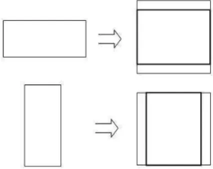
In our experiments, the normalized image plane is set to a square of edge length L, which is not neces-sarily fully occupied. To alleviate the distortion of elongated characters, we partially preserve the as-pect ratio of the input image. By asas-pect ratio adap-tive normalization (ARAN) [29, 36], the aspect ratio R2 of normalized image is a continuous function of
the aspect ratio R1 of input image:
R2= r sin(π 2R1). (3) R1 is calculated by R1= ½ W1/H1, if W1< H1 H1/W1, otherwise (4)
where W1 and H1 are the width and height of the
input image. The width W2 and height H2 of the
normalized image are similarly related by the aspect ratio R2. If the input image is vertically elongated,
then in the normalized plane, the vertical dimension
is filled (height L) and the horizontal dimension is centered and scaled according to the aspect ratio; otherwise, the horizontal dimension is filled (width L) and the vertical dimension is centered and scaled. ARAN is depicted in Fig. 1.
Figure 1: Aspect ratio adaptive normalization (ARAN). Rectangle with thick line: occupied area of normalized image.
The normalization methods depend on the coor-dinate mapping functions, defined by the 1D and pseudo 2D normalization methods as follows.
2.1
1D normalization methods
Given the sizes of input and normalized images, the coordinate mapping functions of linear normaliza-tion (LN) are simply
( x′ = W2 W1x, y′ = H2 H1y. (5)
Both the linear normalization and line-density-based nonlinear normalization (NLN) methods align the physical boundaries (ends of stroke projections) of input image to the boundaries of normalized image. The coordinate mapping of NLN is obtained by ac-cumulating the normalized line density projections (line density equalization):
½
x′ = W2Px
u=0hx(u),
y′ = H2Py
v=0hy(v), (6)
where hx(x) and hy(y) are the normalized line
den-sity histograms of x axis and y axis, respectively, which are obtained by normalizing the projections of local line densities into unity sum:
hx(x) = Ppx(x) xpx(x) = P ydx(x,y) P x P ydx(x,y) , hy(y) = Ppy(y) ypy(y) = P xdy(x,y) P x P ydy(x,y) , (7)
where px(x) and py(y) are the line density
pro-jections onto x axis and y axis, respectively, and dx(x, y) and dy(x, y) are local line density functions.
By Tsukumo and Tanaka [15], the local line den-sities dx and dy are taken as the reciprocal of
hori-zontal/vertical run-length in background area, or a small constant in stroke area. While by Yamada et al. [16], dx and dy are calculated considering
both background run-length and stroke run-length, and are unified to render dx(x, y) = dy(x, y). The
two methods perform comparably but the one of Tsukumo and Tanaka is computationally simpler [5]. By adjusting the density functions of marginal and stroke areas empirically in Tsukumo and Tanaka’s method, we have achieved better performance than the method of Yamada et al. This improved version of NLN is taken in our experiments.
The 1D moment normalization (MN) method (a simplified version of Casey’s method [20]) aligns the centroid of input image (xc, yc) to the geometric
cen-ter of normalized image (x′
c, y′c) = (W2/2, H2/2),
and re-bound the input image according to second-order 1D moments. Let the second-second-order moments be µ20and µ02, the width and height of input image
are re-set to δx = 4√µ20 and δy = 4√µ02,
respec-tively. The coordinate mapping functions are then given by ( x′ = W2 δx(x − xc) + x ′ c, y′ = H2 δy(y − yc) + y ′ c. (8)
The bi-moment normalization (BMN) method [21] aligns the centroid of input image as moment nor-malization does, but the width and height are treated asymmetric with respect to the centroid. To do this, the second-order moments are split into two parts by the centroid: µ−
x, µ+x, µ−y, and µ+y.
The boundaries of input image are re-set to [xc −
2pµ− x, xc+2 p µ+x] and [yc−2 q µ− y, yc+2 q µ+y]. For
the x axis, a quadratic function u(x) = ax2+ bx + c
is used to align three points (xc− 2
p µ−
x, xc, xc +
2pµ+x) to normalized coordinates (0, 0.5, 1), and
similarly, a quadratic function v(y) is used for the y axis. Finally, the coordinate functions are
½
x′ = W 2u(x),
y′ = H
2v(y). (9)
The quadratic functions can also be used to align the physical boundaries and centroid, i.e., map (0, xc, W1) and (0, yc, H1) to (0, 0.5, 1). We call
this method centroid-boundary alignment (CBA). A modified CBA (MCBA) method [22] also adjusts the stroke density in central area by combining a sine function with the quadratic functions:
½
x′ = W
2[u(x) + ηxsin(2πu(x))],
y′ = H
2[v(y) + ηysin(2πv(y))]. (10)
The amplitudes of sine waves, ηx and ηy, are
esti-mated from the extent of the central area, which is defined by the centroids of partial images divided by the global centroid.
2.2
Pseudo 2D normalization
meth-ods
Horiuchi et al. proposed a pseudo 2D nonlinear normalization (P2DNLN) method by equalizing the line density functions of each row/column instead of the line density projections [23]. To control the degree of shape deformation, they blurred the line density functions such that the equalization of each row/column is dependent on its neighboring rows/columns. Though this method promises recog-nition, it is computationally expensive due to the row/column-wise line density blurring.
An efficient pseudo 2D normalization approach, called line density projection interpolation (LDPI), was proposed recently [24]. Instead of line density blurring and row/column-wise equalization, LDPI partitions the 2D line density map into soft strips. 1D coordinate functions are computed from the den-sity projection of each strip and combined to a 2D function. Specifically, let the width and height of the input image be W1and H1, the centroid be (xc, yc),
we partition the horizontal line density map dx(x, y)
into three horizontal strips:
dix(x, y) = wi(y)dx(x, y), i = 1, 2, 3. (11)
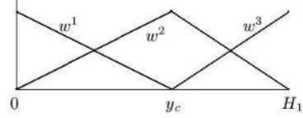
wi(y) (i = 1, 2, 3) are piecewise linear functions:
w1(y) = w 0ycy−y c , y < yc, w2(y) = 1 − w1(y), y < y c, w2(y) = 1 − w3(y), y ≥ y c, w3(y) = w 0Hy−yc 1−yc, y ≥ yc, (12)
where w0controls the weight of the upper/lower part
of line density map. A small value of w0 renders
the interpolated 2D coordinate function close to that of 1D normalization, while a large one may yield excessive deformation. The weight functions with w0= 1 are depicted in Fig. 2.
Figure 2: Weight functions for partitioning line den-sity map into soft strips.
projected onto the x axis: pi x(x) = X y di x(x, y), i = 1, 2, 3. (13)
The projections are then normalized to unity sum and accumulated to give 1D coordinate functions x′i(x), i = 1, 2, 3, which are combined to 2D
co-ordinate function by interpolation:
x′(x, y) = ½ w1(y)x′1(x) + w2(y)x′2(x), y < y c, w3(y)x′3(x) + w2(y)x′2(x), y ≥ y c. (14) Similar to the partitioning of horizontal density, the vertical density map dy(x, y) is partitioned into
three vertical strips using weight functions in x axis. The partitioned density functions di
y(x, y),
i = 1, 2, 3, are similarly equalized and interpolated to generate the 2D coordinate function y′(x, y).
The strategy of LDPI is applied to extend other 1D normalization methods: MN, BMN, and MCBA. The extended versions are called pseudo 2D MN (P2DMN), pseudo 2D BMN (P2DBMN), and pseudo 2D CBA (P2DCBA), respectively. These methods do not rely on the computation of local line density map. Instead, they are directly based on the pixel intensity of character image. As the soft partitioning of line density map in LDPI, the input character image f (x, y) is softly partitioned into three horizontal strips fi
x(x, y), i = 1, 2, 3, and
three vertical strips fi
y(x, y), i = 1, 2, 3. The
hori-zontal strips are projected onto the x axis: pix(x) =
X
y
fxi(x, y), i = 1, 2, 3. (15)
For P2DMN, the second order moment is com-puted from the projection of a strip:
µi 20= P x(x − xic)2pix(x) P xpix(x) . (16)
The width of this strip is re-set to δi
x = 4pµi20,
which is used to determine the scaling factor of 1D coordinate mapping: x′i(x) = W2 δi x (x − xi c) + W2 2 . (17) And the 1D coordinate functions of vertical strips are computed from strip projections similarly.
For P2DBMN, the second order moment of a hor-izontal strip is split into two parts at the centroid of this strip: µi−20 and µi+20. The bounds of this strip
is re-set to [xi c − 2 q µi− 20, xic + 2 q µi+20], which, to-gether with the centroid xi
c, are used to estimate the
quadratic 1D coordinate mapping function x′i(x).
The three 1D coordinate functions of vertical strips are computed similarly.
By P2DCBA, from the vertical projection of each horizontal strip fi
x(x, y) (i = 1, 2, 3), the centroid
coordinate xi
c and two partial centroids xic1and xic2
are computed to estimate the parameters of 1D co-ordinate mapping function x′i(x). Similarly, 1D
co-ordinate functions y′i(y) (i = 1, 2, 3) are estimated
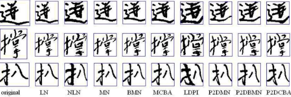
from the horizontal projections of vertical strips. More details of pseudo 2D normalization can be found in [24]. Some examples of normalization using nine methods (LN, NLN, MN, BMN, MCBA, LDPI, P2DMN, P2DBMN, and P2DCBA) are shown in Fig. 3. We can see that whereas linear normaliza-tion (LN) keeps the original shape (only aspect ra-tio changed), NLN can effectively equalize the line intervals. The centroid-based normalization meth-ods (MN, BMN, and MCBA) effectively regulate the overall shape (skewness of gravity, balance of in-ner/outer stroke density). The pseudo 2D methods make the stroke positions more uniform, especially, alleviate the imbalance of width/height and position of character parts.
3
Direction
Feature
Extrac-tion
The implementation of direction feature is vary-ing dependvary-ing on the directional element decompo-sition, the sampling of feature values, the resolu-tion of direcresolu-tion and feature plane, etc. Consider-ing that the stroke segments of Chinese characters can be approximated into four orientations: horizon-tal, vertical, left-diagonal and right-diagonal, early works usually decomposed the stroke (or contour) segments into four orientations.
Feature extraction from stroke contour has been widely adopted because the contour length is nearly independent on stroke-width variation. The local direction of contour, encoded as a chaincode, actu-ally has eight directions (Fig. 4). Decomposing the contour pixels into eight directions instead of four orientations (a pair of opposite directions merged into one orientation) was shown to significantly im-prove the recognition accuracy [26]. This is because separating the two sides of stroke edge can better discriminate parallel strokes. The direction of stroke edge can also be measured by the gradient of image intensity, which applies to gray-scale image as well binary image. The gradient feature has been applied to Chinese character recognition in 8-direction [37] and 12-direction [38].
Figure 3: Character image normalization by nine methods. The leftmost image is original and the other eight are normalized ones.
Figure 4: Eight directions of chaincodes.
three steps: image normalization, directional de-composition, and feature sampling. Convention-ally, the contour/edge pixels of normalized im-age are assigned to a number of direction planes. The normalization-cooperated feature extraction (NCFE) strategy [25], instead, assigns the chain-codes of original image into direction planes. Though the normalized image is not generated by NCFE, the coordinates of pixels in original image are mapped to a standard plane, and the extracted fea-ture is thus dependent on the normalization method. Direction feature is also called direction histogram feature because at a pixel or a local region in nor-malized image, the strength values of Nd directions
form a local histogram. Alternatively, we view the strength values of one direction as a directional im-age (direction plane).
In the following, we first describe the direc-tional decomposition procedures for three types of direction features: chaicode direction fea-ture, normalization-cooperated chaincode feature (NCCF), and gradient direction feature, and then address the sampling of direction planes.
3.1
Directional decomposition
Directional decomposition results in a number of di-rection planes (with same size as the normalize im-age), fi(x, y), i = 1, . . . , Nd. We first describe the
procedures for decomposing contour/gradient into
eight directions, then extend to 12 directions and 16 directions.
In binary image, a contour pixel is a black point with at least one of its 4-connected neighbors being white. The 8-direction chaincodes of contour pixels can be decided by contour tracing, or more simply, by raster scan [39]. At a black pixel (x, y), denot-ing the values of 8-connected neighbors in counter-clockwise as pk, 0, 1, . . . , 7, with the east neighbor
being p0. For k = 0, 2, 4, 6, if pk = 0, check pk+1: if
pk+1= 1 (chaincode k + 1), fk+1(x, y) increases by
1; otherwise, if p(k+2)%8= 1 (chaincode (k + 2)%8),
f(k+2)%8(x, y) increases by 1.
For NCCF, each chaincode in the original image is viewed as a line segment connecting two neighboring pixels, which is mapped to another line segment in a standard direction plane by coordinate mapping. In the direction plane, each pixel (unit square) crossed by the line segment in the main (x or y) direction is given a unit of direction contribution. To exploit the continuous nature of line segment, the strength of line direction falling in a pixel is proportional to the length of line segment falling in the unit square (continuous NCCF [29]). As in Fig. 5, where a line segment mapped from a chaincode covers four unit squares A, B, C and D. By discrete NCCF, the pixels A and C are assigned a direction unit, whereas by continuous NCCF, all the four pixels are assigned direction strengths proportional to the in-square line segment length.
Figure 5: NCCF on continuous direction plane. In gradient direction feature extraction, the
gradi-ent vector, computed on the normalized image using the Sobel operator, is decomposed into components in eight chaincode directions. The Sobel operator has two masks to compute the gradient components in two axes. The masks are shown in Fig. 6, and the gradient g(x, y) = [gx, gy]T at location (x, y) is
computed by gx(x, y) = f (x + 1, y − 1) + 2f(x + 1, y) + f(x + 1, y + 1) −f(x − 1, y − 1) − 2f(x − 1, y) + f(x − 1, y + 1), gy(x, y) = f (x − 1, y + 1) + 2f(x, y + 1) + f(x + 1, y + 1) −f(x − 1, y − 1) − 2f(x, y − 1) + f(x + 1, y − 1). (18)
Figure 6: Templates of Sobel gradient operator. The gradient strength and direction can be com-puted from the vector [gx, gy]T. The range of
gradi-ent direction can be partitioned into a number (say, 8 or 16) of regions and each region corresponds to a direction plane. More effectively, the gradient vec-tor is decomposed into components in standard di-rections, following a strategy previously proposed in online character recognition [27]. In this scheme, if a gradient direction lies between two standard direc-tions, the vector is decomposed into two components as shown in Fig. 7. The length of each component is assigned to the corresponding direction plane at the pixel (x, y).
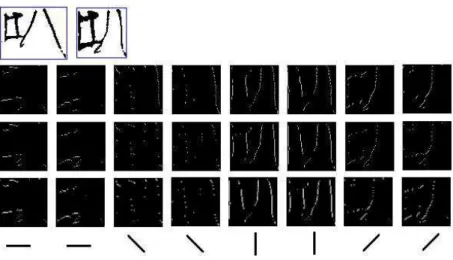
Figure 7: Decomposition of gradient vector. Fig. 8 shows the direction planes of three decom-position schemes: NCCF, chaincodes of normaliza-tion image, and gradient of normalized image. The direction planes are arranged in the order of stroke orientation. We can see that the planes of chain-code directions (third row) are very similar to those of gradient directions. The planes of NCCF, de-scribing the local directions of original image, show
some difference. Comparing the original image and the normalized image, the orientation of the right-hand stroke, near left-diagonal orientation, deforms to near vertical. Consequently, the direction planes of left-diagonal orientation of NCCF are stronger than those of chaincodes and gradient, while the planes of vertical orientation of NCCF are weaker than those of chaincodes and gradient.
3.2
Extention to more directions
The extension of gradient decomposition into more than eight directions is straightforward: simply setting Nd standard directions with angle interval360/Nd and typically, with one direction pointing
to east, then decompose each gradient vector into two components in standard directions and assign the component lengths to corresponding direction planes. We set Nd to 12 and 16.
To decompose contour pixels into 16 directions follows the 16-direction extended chaincodes, which is defined by two consecutive chaincodes. In the weighted direction histogram feature of Kimura et al. [18], 16-direction chaincodes are down-sampled by weighted average to form 8-direction planes.
Again, we can determine the 16-direction chain-code of contour pixels by raster scan. At a contour pixel (x, y), when its 4-connected neighbor pk = 0
and the counterclockwise successor pk+1 = 1 or
p(k+2)%2 = 1, search the neighbors clockwise from
pk until a pj = 1 is found. The two contour pixels,
pk+1 or p(k+2)%2 and pj, form a 16-direction
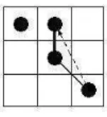
chain-code. For example, in Fig. 9, the center pixel has the east neighbor being 0, the north neighbor alone defining the 8-direction chaincode, and defining a 16-direction chaincode together with the southeast neighbor. The 16-direction chaincode can be in-dexed from a table of correspondence between the code and the difference of coordinates of two pixels forming the code, as shown in Fig. 10. Each contour pixel has a unique 16-direction code.
Figure 9: 16-direction chaincode formed from two 8-direction chaincodes.
For decomposing contour pixels into 12 directions, the difference of coordinates corresponding to a 16-direction chaincode is viewed as a vector (the dashed line in Fig. 9), which is decomposed into compo-nents in 12 standard directions as a gradient vector
Figure 8: Original image and normalized image (top row), 8-direction planes of NCCF (second row), chain-code planes of normalized image (third row), and gradient direction planes (bottom row).
Figure 10: Difference of coordinates and the corre-sponding 16-direction chaincodes.
is done. In this sense, the 12-direction code of a con-tour pixel is not unique. For 12-direction chaincode feature extraction, a contour pixel is assigned to two direction planes, with strength proportional to the component length. For NCCF, the two correspond-ing direction planes are assigned strengths propor-tional to the overlapping length of the line segment mapped by coordinate functions, as in Fig. 5.
3.3
Blurring and sampling
Each direction plane, with same size as the normal-ized image, need to be reduced to extract feature val-ues of moderate dimensionality. A simple way is to partition the direction plane into a number of block zones and take the total or average value of each zone as a feature value. Partition of variable-size zones was proposed to overcome the non-uniform distri-bution of stroke density [13], but is not necessary when nonlinear or pseudo 2D normalization is done. Overlapping blocks were taken to alleviate the ef-fect of stroke-position variation on the boundary of blocks [40], yet a more effective way is to partition
the plane into soft zones, which follow the princi-ple of low-pass spatial filtering and sampling [39]. The blurring operation of Iijima [11] implies spatial filtering without down-sampling.
In implementation of blurring, the impulse re-sponse function (IRF) of spatial filter is approxi-mated into a weighted window, which is also called a blurring mask. The IRF is often taken as a Gaussian function: h(x, y) = 1 2πσ2 x exp³−x 2+ y2 2σ2 x ´ . (19)
According to the Sampling Theorem, the variance parameter σx is related to the sampling frequency
(the reciprocal of sampling interval). On truncat-ing the band-width of Gaussian filter, an empirical formula was given in [39]:
σx=
√ 2tx
π , (20)
where tx is the sampling interval. At a location
(x0, y0) of image f (x, y), the convolution gives a
sampled feature value F (x0, y0) = X x X y f (x, y) · h(x − x0, y − y0). (21)
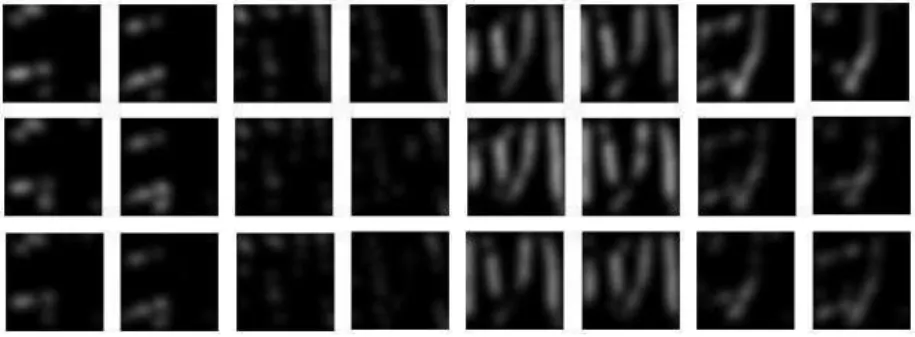
Fig. 11 show the blurred images (without down-sampling) of the direction planes in Fig. 8. By blur-ring, the sparse pixels in direction planes merge into strokes or blobs.
For ease of implementation, we partition a direc-tion plane into a mesh of equal-size blocks and set the sampling points to the center of each block. As-sume to extract K × K values from a plane, the size of plane is set to Ktx × Ktx. From Nd direction
Figure 11: Blurred images (not down-sampled) of the direction planes in Fig. 8.
planes, the total number of extracted feature values is Nd× K2.
The extracted feature values are causal variables. Power transformation can make the density func-tion of causal variables closer to Gaussian [7]. This is helpful to improve the classification performance of statistical classifiers. Power transformation is also called variable transformation [41] or Box-Cox trans-formation [42]. We transform each feature value with power 0.5 without attempt to optimize the transformation functions.
4
Performance Evaluation
We first compare the performance of the normaliza-tion and feature extracnormaliza-tion methods on two large databases of handprinted characters (constrained writing), and then test the performance on a small set of unconstrained handwritten characters.
We use two classifiers for classification: the Eu-clidean distance to class mean (minimum distance classifier) and the MQDF [17]. For reducing the classifier complexity and improving classification ac-curacy, the feature vector is transformed to a lower dimensionality by Fisher linear discriminant analy-sis (FLDA) [7]. We set the reduced dimensionality to 160 for all feature types.
Denote the d-dimensional feature vector (after di-mensionality reduction) by x, the MQDF of class ωi
is computed by g2(x, ωi) =Pkj=1 1 λij[(x − µi) Tφ ij]2 +δ1 i n kx − µik2−Pkj=1[(x − µi)Tφij]2 o +Pk j=1log λij+ (d − k) log δi, (22) where µi is the mean vector of class ωi, λij and
φij, j = 1, . . . , d, are the eigenvalues and
eigen-vectors of the covariance matrix of class ωi. The
eigenvalues are sorted in non-ascending order and the eigenvectors are sorted accordingly. k denotes
the number of principal axes, and the minor eigen-values are replaced with a constant δi. We set a
class-independent constant δi which is proportional
to the average feature variance, with the multiplier selected by 5-fold holdout validation on the training data set.
In our experiments, k was set to 40. The classifica-tion of MQDF is speeded up by selecting 100 candi-date classes using Euclidean distance. The MQDF is then computed on the candidate classes only. Candi-date selection is further accelerated by clustering the class means into groups. The input feature vector is first compared to cluster centers, and then compared to the class means contained in a number of near-est clusters. We set the total number of clusters to 220 for the ETL9B database and 250 for the CASIA database.
MQDF is a promising classification method for HCCR. Even higher performance can be achieved by, e.g., discriminative learning of feature transfor-mation and classifier parameters [37, 38]. The opti-mization of classifier, however, is not the concern of this paper.
4.1
Performance
on
handprinted
characters
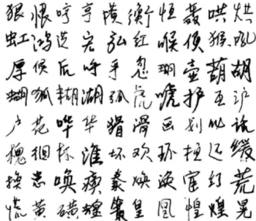
The normalization and feature extraction methods are evaluated on two databases of handprinted char-acters. The ETL9B database contains the character images of 3,036 classes (71 hiragana, and 2,965 Kanji characters in the JIS level-1 set), 200 samples per class. This database has been widely evaluated by the community [18, 40, 43]. The CASIA database, collected by the Institute of Automation, Chinese Academy of Sciences, in early 1990s, contains the handwritten images of 3,755 Chinese characters (the level-1 set in GB2312-80 standard), 300 samples per class. Some sample images of the CASIA database are shown in Fig. 12.
In the ETL9B database, we use the first 20 and last 20 samples of each class for testing, and the
re-Figure 12: Test samples in the CASIA database.
maining samples for training classifiers. In the CA-SIA database, we use the first 250 samples of each class for training, and the remaining 50 samples per class for testing.
We first compare the performance of three direc-tion features with varying direcdirec-tion resoludirec-tions with a common normalization method (Tsukumo and Tanaka’s nonlinear normalization (NLN) method with our modifications). The direction resolution of features is set to 8, 12, and 16. For each direc-tion resoludirec-tion, three schemes of sampling mesh are tested. For 8-direction features, the mesh of sam-pling is set to 7×7 (M1), 8×8 (M2), and 9×9 (M3); for 12-direction, 6 × 6 (M1), 7 × 7 (M2), and 8 × 8 (M3); and for 16-direction, 5 × 5 (M1), 6 × 6 (M2), and 7 × 7 (M3). We control the size of normalized image (direction planes) to be around 64 × 64, and the dimensionality (before reduction) to be less than 800. The settings of sampling mesh are summarized in Table 1.
Table 1: Settings of sampling mesh for 8-direction, 12-direction, and 16-direction features.
Mesh M1 M2 M3
zones dim zones dim zones dim 8-dir 7 × 7 392 8 × 8 512 9 × 9 648 12-dir 6 × 6 432 7 × 7 588 8 × 8 768 16-dir 5 × 5 400 6 × 6 576 7 × 7 784
On classifier training and testing using different direction resolutions and sampling schemes, the er-ror rates on the test set of ETL9B database are listed in Table 2, and the error rates on the test set of CA-SIA database are listed in Table 3. In the tables, the chaincode direction feature is denoted by chn, NCCF is denoted by nccf, and the gradient
direc-Table 2: Error rates (%) of 8-direction, 12-direction, and 16-direction features on ETL9B database.
Euclidean MQDF chn M1 M2 M3 M1 M2 M3 8-dir 2.91 2.94 3.02 1.08 1.05 1.09 12-dir 2.43 2.56 2.54 1.02 1.00 0.97 16-dir 2.52 2.40 2.52 1.20 1.00 1.00 nccf M1 M2 M3 M1 M2 M3 8-dir 2.61 2.61 2.71 0.93 0.87 0.89 12-dir 2.05 2.06 2.13 0.82 0.77 0.78 16-dir 2.05 2.04 2.11 0.98 0.85 0.79 grd-g M1 M2 M3 M1 M2 M3 8-dir 2.59 2.58 2.66 0.93 0.90 0.89 12-dir 2.27 2.30 2.31 0.94 0.86 0.86 16-dir 2.29 2.19 2.25 1.08 0.94 0.85
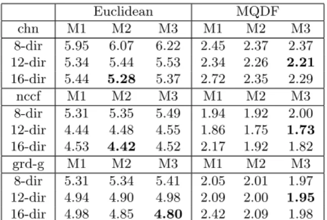
Table 3: Error rates (%) of 8-direction, 12-direction, and 16-direction features on CASIA database.
Euclidean MQDF chn M1 M2 M3 M1 M2 M3 8-dir 5.95 6.07 6.22 2.45 2.37 2.37 12-dir 5.34 5.44 5.53 2.34 2.26 2.21 16-dir 5.44 5.28 5.37 2.72 2.35 2.29 nccf M1 M2 M3 M1 M2 M3 8-dir 5.31 5.35 5.49 1.94 1.92 2.00 12-dir 4.44 4.48 4.55 1.86 1.75 1.73 16-dir 4.53 4.42 4.52 2.17 1.92 1.82 grd-g M1 M2 M3 M1 M2 M3 8-dir 5.31 5.34 5.41 2.05 2.01 1.97 12-dir 4.94 4.90 4.98 2.09 2.00 1.95 16-dir 4.98 4.85 4.80 2.42 2.09 1.98
tion feature by grd-g. For chaincode feature extrac-tion, the normalized binary image is smoothed using a connectivity-preserving smoothing algorithm [39]. Gradient feature is extracted from gray-scale nor-malized image.
We can see that on either database, using either classifier (Euclidean or MQDF), the error rates of 12-direction and 16-12-direction features are mostly lower than those of 8-direction features. This indicates that increasing the resolution of direction decompo-sition is beneficial. The 16-direction feature, how-ever, does not outperform the 12-direction feature. To select a sampling mesh, let us focus on the re-sults of 12-direction features. We can see that by Euclidean distance classification, M1 (6 × 6) outper-forms M2 (7×7) and M3 (8×8), whereas by MQDF, the error rates of M2 and M3 are lower than those of M1. Considering that M2 and M3 perform com-parably while M2 has lower complexity, we take the sampling mesh M2 with 12-direction features for
fol-lowing experiments. The original dimensionality of direction features is now 12 × 7 × 7 = 588.
Table 4: Error rates (%) of various normalization methods on ETL9B database.
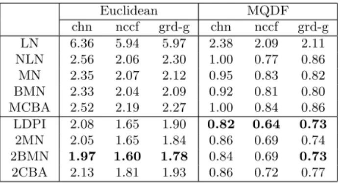
Euclidean MQDF chn nccf grd-g chn nccf grd-g LN 6.36 5.94 5.97 2.38 2.09 2.11 NLN 2.56 2.06 2.30 1.00 0.77 0.86 MN 2.35 2.07 2.12 0.95 0.83 0.82 BMN 2.33 2.04 2.09 0.92 0.81 0.80 MCBA 2.52 2.19 2.27 1.00 0.84 0.86 LDPI 2.08 1.65 1.90 0.82 0.64 0.73 2MN 2.05 1.65 1.84 0.86 0.69 0.74 2BMN 1.97 1.60 1.78 0.84 0.69 0.73 2CBA 2.13 1.81 1.93 0.86 0.72 0.77
Table 5: Error rates (%) of various normalization methods on CASIA database.
Euclidean MQDF chn nccf grdg chn nccf grd-g LN 11.38 10.46 10.31 4.11 3.49 3.54 NLN 5.44 4.48 4.90 2.26 1.75 2.00 MN 5.61 4.89 4.90 2.50 2.04 2.06 BMN 5.30 4.54 4.56 2.35 1.93 1.92 MCBA 5.48 4.73 4.83 2.31 1.87 1.96 LDPI 4.49 3.69 4.21 1.96 1.52 1.75 2MN 4.99 3.97 4.33 2.24 1.70 1.91 2BMN 4.63 3.71 4.07 2.15 1.62 1.76 2CBA 4.75 3.95 4.25 2.11 1.68 1.78
On fixing the direction resolution (12-direction) and sampling mesh (7 × 7), we combine the three types of direction features with nine normalization methods. The weight parameter w0 of pseudo 2D
normalization was set to 0.75 for good recognition performance [24]. The error rates on the test sets of two databases are listed in Table 4 and Table 5, respectively. In the tables, the pseudo 2D normal-ization methods P2DMN, P2DBMN, and P2DCBA are denoted by 2MN, 2BMN, and 2CBA, respec-tively, for saving space. Comparing the normaliza-tion methods, we can see that pseudo 2D methods are superior to 1D ones, and the linear normaliza-tion (LN) is inferior to other 1D normalizanormaliza-tion meth-ods. To compare the three types of features, let us view the error rates of 1D normalization methods and those of pseudo 2D methods separately.
It can be seen in Table 4 and Table 5 that with 1D normalization, the NCCF and the gradient
fea-ture perform comparably, and both outperform the chaincode feature. Four normalization methods, namely, NLN, MN, BMN, and MCBA, perform com-parably. With pseudo 2D normalization, the NCCF perform best, and the gradient feature outperforms the chaincode feature. Comparing the pseudo 2D normalization methods, LDPI and P2DBMN out-perform P2DMN and P2DCBA (especially on the CASIA database). On both two databases, the best performance is yielded by the NCCF with LDPI nor-malization, and the NCCF with P2DBMN is com-peting.
The gradient feature performs comparably with NCCF with 1D normalization but inferiorly with pseudo 2D normalization. This is because pseudo 2D normalization, though equalize the stroke den-sity better than 1D normalization, also deforms the stroke directions remarkably. While the gradi-ent feature describes the deformed stroke directions, NCCF takes the stroke directions of original image.
4.2
Computation times
To compare the computational complexity of nor-malization methods, we profile the processing time in two sub-tasks: coordinate mapping and normal-ized image generation, and the latter is dichotomnormal-ized into binary image and gray-scale image. Smoothing is involved in binary normalized image, but not for gray-scale image.
On the test samples of CASIA database, we counted the CPU times on Pentium-4-3GHz proces-sor. The average times per sample are shown in Ta-ble 6. We can see that the processing time of coordi-nate mapping varies with the normalization method. The linear normalization (LN) is very fast. NLN is more expensive than other 1D methods, and LDPI is more expensive than other pseudo 2D methods. This is because NLN and LDPI involve line density computation. Nevertheless, all these normalization methods are not computationally expensive. Nor-malized image generation for pseudo 2D normaliza-tion methods is very time consuming because it in-volves quadrilateral decomposition. The processing time of binary normalized image includes a smooth-ing time of about 0.3ms.
The CPU time of feature extraction is almost independent of normalization method. It has two parts: directional decomposition and blurring. The average CPU times of three direction features are shown in Table 7. The processing time of blurring depends on the sparsity of direction planes (zero pixels are not considered). The direction planes of chaincode feature are sparse, and those of
gra-Table 6: Average CPU times (ms) of normalization on CASIA database. Binary normalized image in-volves smoothing.
coordinate binary grayscale LN 0.002 0.318 0.133 NLN 0.115 0.331 0.143 MN 0.017 0.321 0.126 BMN 0.024 0.332 0.135 MCBA 0.032 0.336 0.137 LDPI 0.266 1.512 1.282 P2DMN 0.143 1.514 1.236 P2DBMN 0.147 1.536 1.274 P2DCBA 0.156 1.542 1.261
dient feature are densest. The directional decom-position of NCCF is most time-consuming because it involves line segment decomposition, and gradi-ent direction decomposition is more expensive than chaincode decomposition. Overall, NCCF is still the most computationally efficient because it saves the time of normalized image generation. The av-erage CPU time of NCCF ranges from 1.21ms to 1.47ms, covering coordinate mapping and feature extraction. For reference, the average classification time of MQDF (with cluster-based candidate selec-tion) for 3,755 classes is 3.63ms, which can be largely reduced by fine implementation, however.
Table 7: Average CPU times (ms) of feature extrac-tion on CASIA database.
direction blurring chn 0.121 0.439 nccf 0.458 0.752 grd-g 0.329 1.276
4.3
Performance
on
unconstrained
handwriting
The error rates of the best methods on handprinted characters, say, 0.64% on ETL9B database and 1.52% on CASIA database, are fairly high. To test the performance on unconstrained handwritten characters, we use the classifiers trained with the training set of CASIA database to classify the sam-ples in a small data set, which contains 20 samsam-ples for each of 3,755 classes, written by 20 writers with-out constraint. Some samples of the unconstrained set are shown in Fig. 13.
On the unconstrained set, we evaluate various
nor-Figure 13: Samples of unconstrained handwritten characters.
malization methods with two good features: NCCF and gradient direction feature. The error rates are listed in Table 8. We can see that as for handprinted characters, the pseudo 2D normaliza-tion methods yield lower error rates than their 1D counterparts on unconstrained characters as well. However, line-density-based nonlinear normalization methods, NLN and LDPI, are evidently inferior to the centroid-based methods. The P2DBMN method performs best, and the P2DCBA method is competi-tive. Comparing the two types of direction features, the gradient features outperforms NCCF with 1D normalization methods, but with pseudo 2D normal-ization, NCCF is superior. Overall, the error rates on unconstrained characters are still very high.
Table 8: Error rates (%) on unconstrained handwrit-ten Chinese characters.
Euclidean MQDF nccf grdg nccf grd-g LN 36.04 35.44 21.80 21.46 NLN 26.61 27.04 16.23 16.96 MN 25.63 25.18 16.40 16.09 BMN 25.15 24.53 15.91 15.64 MCBA 25.53 25.06 15.76 15.66 LDPI 24.93 25.60 15.12 15.73 P2DMN 23.48 24.38 14.84 15.37 P2DBMN 22.75 23.35 14.27 14.64 P2DCBA 23.80 23.78 14.73 14.79
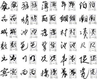
Fig. 14 shows some misclassified samples by MQDF with the best normalization-feature combi-nation (P2DBMN and NCCF). Most of the misclas-sified characters are similar in shape to the assigned class: some are inherently similar (top three rows in Fig. 14), and some others are similar due to cursive writing (fourth and fifth rows). Yet the characters
of the bottom row are not highly similar to their assigned classes.
Figure 14: Misclassified samples (each shown origi-nal image and normalized image) of unconstrained handwritten characters.
5
Concluding Remarks
We compared various shape normalization and se-lected feature extraction methods in offline hand-written Chinese character recognition. For direction feature extraction, our results show that 12-direction and 16-direction features outperform 8-direction fea-ture, and the 12-direction feature has better trade-off between accuracy and complexity. The compari-son of normalization methods shows that pseudo 2D normalization methods outperform their 1D coun-terparts. On handprinted characters, a line-density-based method LDPI and a centroid-line-density-based method P2DBMN perform best. Comparing three types of direction features, the NCCF and the gradient feature outperform the chaincode feature, compete when 1D normalization is used, but with pseudo 2D normalization, the NCCF outperforms the gradi-ent feature. Overall, the best normalization-feature combinations are LDPI and P2DBMN with NCCF. We also tested the performance on a small set of unconstrained handwritten characters, with clas-sifiers trained with handprinted samples. The er-ror rates on unconstrained characters are very high, but the comparison of normalization and feature extraction methods reveals new insights. Though pseudo 2D normalization methods again outperform their 1D counterparts, the line-density-based LDPI method is inferior to the centroid-based methods, and the P2DBMN method performs best. The best
normalization-feature combination on unconstrained characters is P2DBMN with NCCF.
Training classifiers with unconstrained handwrit-ten samples will be able to improve the accuracy of unconstrained character recognition. To collect large database of unconstrained characters is an ur-gent task in the near future. To reduce the error rate to a fairly low level (say, 2% on isolated char-acters), however, simply using the current normal-ization and feature extraction methods and train-ing current classifiers with larger sample set will not suffice. The methods of shape normalization, fea-ture extraction, and classifier design need to be re-considered for better recognizing cursively written characters. Training classifiers discriminatively can improve the accuracy of both handprinted and un-constrained character recognition.
Acknowledgements
This work is supported in part by the Hundred Talents Program of Chinese Academy of Sciences and the Natural Science Foundation of China (grant no.60543004).
References
[1] R. Casey and G. Nagy, Recognition of printed Chinese Characters, IEEE Trans. Electronic Computers 15(1) (1966) 91-101.
[2] W. Stalling, Approaches to Chinese character recognition, Pattern Recognition 8 (1976) 87-98.
[3] S. Mori, K. Yamamoto, and M. Yasuda, Re-search on machine recognition of handprinted characters, IEEE Trans. Pattern Anal. Mach. Intell.6(4) (1984) 386-405.
[4] T.H. Hildebrandt and W. Liu, Optical recogni-tion of Chinese characters: advances since 1980, Pattern Recognition 26(2) (1993) 205-225. [5] M. Umeda, Advances in recognition methods
for handwritten Kanji characters, IEICE Trans. Information and Systems E29(5) (1996) 401-410.
[6] C.-L. Liu, S. Jaeger, and M. Nakagawa, Online recognition of Chinese characters: the state-of-the-art, IEEE Trans. Pattern Anal. Mach. In-tell.26(2) (2004) 198-213.
[7] K. Fukunaga, Introduction to Statistical Pat-tern Recognition, 2nd edition (Academic Press, 1990).
[8] R.O. Duda, P.E. Hart, and D.G. Stork, Pattern Classification, 2nd edition (Wiley Interscience, 2001).
[9] A.K. Jain, R.P.W. Duin, and J. Mao, Statisti-cal pattern recognition: a review, IEEE Trans. Pattern Anal. Mach. Intell.22(1) (2000) 4-37. [10] I.-J. Kim and J.H. Kim, Statistical character structure modeling and its application to hand-written Chinese character recognition, IEEE Trans. Pattern Anal. Mach. Intell. 25(11) (2003) 1422-1436.
[11] T. Iijima, H. Genchi, and K. Mori, A theoretical study of the pattern identification by matching method, in Proc. First USA-JAPAN Computer Conference, Oct. 1972, 42-48.
[12] M. Yasuda and H. Fujisawa, An improvement of correlation method for character recognition, Trans. IEICE JapanJ62-D(3) (1979) 217-224 (in Japanese).
[13] Y. Yamashita, K. Higuchi, Y. Yamada, and Y. Haga, Classification of handprinted Kanji characters by the structured segment matching method, Pattern Recognition Letters 1 (1983) 475-479.
[14] H. Fujisawa and C.-L. Liu, Directional pattern matching for character recognition revisited, in Proc. 7th Int’l Conf. on Document Analysis and Recognition, Edinburgh, Scotland, 2003, 794-798.
[15] J. Tsukumo and H. Tanaka, Classification of handprinted Chinese characters using non-linear normalization and correlation methods, in Proc. 9th Int’l Conf. on Pattern Recognition, Rome, 1988, 168-171.
[16] H. Yamada, K. Yamamoto, and T. Saito, A nonlinear normalization method for hanprinted Kanji character recognition—line density equal-ization, Pattern Recognition 23(9) (1990) 1023-1029.
[17] F. Kimura, K. Takashina, S. Tsuruoka, and Y. Miyake, Modified quadratic discriminant func-tions and the application to Chinese character recognition, IEEE Trans. Pattern Anal. Mach. Intell.9(1) (1987) 149-153.
[18] F. Kimura, T. Wakabayashi, S. Tsuruoka, and Y. Miyake, Improvement of handwritten Japanese character recognition using weighted direction code histogram, Pattern Recognition 30(8) (1997) 1329-1337.
[19] N. Kato, M. Abe, Y. Nemoto, A handwrit-ten character recognition system using modi-fied Mahalanobis distance, Trans. IEICE Japan J79-D-II(1) (1996) 45-52.
[20] R.G. Casey, Moment normalization of hand-printed character, IBM J. Res. Develop. 14 (1970) 548-557.
[21] C.-L. Liu, H. Sako, and H. Fujisawa, Handwrit-ten Chinese character recognition: alternatives to nonlinear normalization, in Proc. 7th Int’l Conf. on Document Analysis and Recognition, Edinburgh, Scotland, 2003, 524-528.
[22] C.-L. Liu and K. Marukawa, Global shape nor-malization for handwritten Chinese character recognition: a new method, in Proc. 9th Int’l Workshop on Frontiers of Handwriting Recog-nition, Tokyo, Japan, 2004, 300-305.
[23] T. Horiuchi, R. Haruki, H. Yamada, and K. Ya-mamoto, Two-dimensional extension of nonlin-ear normalization method using line density for character recognition, in Proc. 4th Int’l Conf. on Document Analysis and Recognition, Ulm, Germany, 1997, 511-514.
[24] C.-L. Liu and K. Marukawa, Pseudo two-dimensional shape normalization methods for handwritten Chinese character recognition, Pattern Recognition 38(12) (2005) 2242-2255. [25] M. Hamanaka, K. Yamada, and J. Tsukumo,
Normalization-cooperated feature extraction method for handprinted Kanji character recog-nition, in Proc. 3rd Int’l Workshop on Frontiers of Handwriting Recognition, Buffalo, NY, 1993, 343-348.
[26] C.-L. Liu, K. Nakashima, H. Sako, and H. Fu-jisawa, Handwritten digit recognition: bench-marking of state-of-the-art techniques, Pattern Recognition36(10) (2003) 2271-2285.
[27] A. Kawamura, K. Yura, T. Hayama, Y. Hidai, T. Minamikawa, A. Tanaka, and S. Ma-suda, On-line recognition of freely handwrit-ten Japanese characters using directional fea-ture densities, in Proc. 11th Int’l Conf. on Pat-tern Recognition, The Hague, 1992, Vol.2, 183-186.
[28] G. Srikantan, S.W. Lam, and S.N. Srihari, Gradient-based contour encoder for character recognition, Pattern Recognition 29(7) (1996) 1147-1160.
[29] C.-L. Liu, K. Nakashima, H. Sako, and H. Fu-jisawa, Handwritten digit recognition: investi-gation of normalization and feature extraction techniques, Pattern Recognition 37(2) (2004) 265-279.
[30] N. Hagita, S. Naito, and I. Masuda, Hand-printed Chinese characters recognition by pe-ripheral direction contributivity feature, Trans. IEICE JapanJ66-D(10) (1983) 1185-1192 (in Japanese).
[31] M. Yasuda, K. Yamamoto, H. Yamada, and T. Saito, An improved correlation method for handprinted Chinese character recognition in a reciprocal feature field, Trans. IEICE Japan J68-D(3) (1985) 353-360.
[32] L.-N. Teow and K.-F. Loe, Robust vision-based features and classification schemes for off-line handwritten digit recognition, Pattern Recog-nition35(11) (2002) 2355-2364.
[33] M. Shi, Y. Fujisawa, T. Wakabayashi, and F. Kimura, Handwritten numeral recognition us-ing gradient and curvature of gray scale image, Pattern Recognition35(10) (2002) 2051-2059. [34] X. Wang, X. Ding, and C. Liu, Gabor
filter-base feature extraction for character recogni-tion, Pattern Recognition 38(3) (2005) 369-379. [35] C.-L. Liu, M. Koga, and H. Fujisawa, Ga-bor feature extraction for character recognition: comparison with gradient feature, in Proc. 8th Int’l Conf. on Document Analysis and Recogni-tion, Seoul, Korea, 2005, 121-125.
[36] C.-L. Liu, M. Koga, and H. Sako, H. Fujisawa, Aspect ratio adaptive normalization for hand-written character recognition, in Advances in Multimodal Interfaces—ICMI2000, T. Tan, Y. Shi, W. Gao (Eds.), LNCS Vol. 1948, Springer, 2000, 418-425.
[37] C.-L. Liu, High accuracy handwritten Chinese character recognition using quadratic classifiers with discriminative feature extraction, in Proc. 18th Int’l Conf. on Pattern Recognition, Hong Kong, 2006, Vol.2, 942-945.
[38] H. Liu and X. Ding, Handwritten charac-ter recognition using gradient feature and
quadratic classifier with multiple discrimination schemes, in Proc. 8th Int’l Conf. on Document Analysis and Recognition, Seoul, Korea, 2005, 19-23.
[39] C.-L. Liu, Y-J. Liu, and R-W. Dai, Prepro-cessing and statistical/structural feature ex-traction for handwritten numeral recognition, in Progress of Handwriting Recognition, A.C. Downton and S. Impedovo (Eds.), (World Sci-entific, 1997) 161-168.
[40] J. Guo, N. Sun, Y. Nemoto, M. Kimura, H. Echigo, and R. Sato, Recognition of hand-written characters using pattern transforma-tion method with cosine functransforma-tion, Trans. IE-ICE Japan J76-D-II(4) (1993) 835-842 (in Japanese).
[41] T. Wakabayashi, S. Tsuruoka, F. Kimura, and Y. Miyake, On the size and variable transfor-mation of feature vector for handwritten char-acter recognition, Trans. IEICE Japan J76-D-II(12) (1993) 2495-2503 (in Japanese). [42] R.V.D. Heiden, and F.C.A. Gren, The Box-Cox
metric for nearest neighbor classification im-provement, Pattern Recognition 30(2) (1997) 273-279.
[43] N. Kato, M. Suzuki, S. Omachi, H. Aso, and Y. Nemoto, A handwritten character recog-nition system using directional element fea-ture and asymmetric Mahalanobis distance, IEEE Trans. Pattern Anal. Mach. Intell.21(3) (1999) 258-262.