Temporal-spatial structure of magnetic merging at the magnetopause inferred from 557.7-nm all-sky images

HAL Id: hal-00317591

https://hal.archives-ouvertes.fr/hal-00317591

Submitted on 7 Sep 2004

HAL is a multi-disciplinary open access

archive for the deposit and dissemination of

sci-entific research documents, whether they are

pub-lished or not. The documents may come from

teaching and research institutions in France or

abroad, or from public or private research centers.

L’archive ouverte pluridisciplinaire HAL, est

destinée au dépôt et à la diffusion de documents

scientifiques de niveau recherche, publiés ou non,

émanant des établissements d’enseignement et de

recherche français ou étrangers, des laboratoires

publics ou privés.

magnetopause inferred from 557.7-nm all-sky images

N. C. Maynard, J. Moen, W. J. Burke, M. Lester, D. M. Ober, J. D. Scudder,

K. D. Siebert, D. R. Weimer, C. T. Russell, A. Balogh

To cite this version:

N. C. Maynard, J. Moen, W. J. Burke, M. Lester, D. M. Ober, et al.. Temporal-spatial structure of

magnetic merging at the magnetopause inferred from 557.7-nm all-sky images. Annales Geophysicae,

European Geosciences Union, 2004, 22 (8), pp.2917-2942. �hal-00317591�

SRef-ID: 1432-0576/ag/2004-22-2917 © European Geosciences Union 2004

Annales

Geophysicae

Temporal-spatial structure of magnetic merging at the

magnetopause inferred from 557.7-nm all-sky images

N. C. Maynard1, J. Moen2, W. J. Burke3, M. Lester4, D. M. Ober1, J. D. Scudder5, K. D. Siebert1, D. R. Weimer1, C. T. Russell6, and A. Balogh7

1_{ATK Mission Research, Nashua, New Hampshire, USA} 2_{University of Oslo, Oslo, Norway}

3_{Air Force Research Laboratory, Hanscom Air Force Base, Massachusetts, USA} 4_{University of Leicester, Leicester, UK}

5_{Department of Physics and Astronomy, University of Iowa, Iowa City, Iowa, USA} 6_{University of California at Los Angeles, Los Angeles, CA, USA}

7_{Imperial College, Exhibition Road, London, SW7 2BW, UK}

Received: 18 September 2003 – Revised: 18 March 2004 – Accepted: 8 April 2004 – Published: 7 September 2004

Abstract. We demonstrate that high-resolution 557.7-nm all-sky images are useful tools for investigating the spatial and temporal evolution of merging on the dayside magne-topause. Analysis of ground and satellite measurements leads us to conclude that high-latitude merging events can oc-cur at multiple sites simultaneously and vary asynchronously on time scales of 30 s to 3 min. Variations of 557.7 nm emis-sions were observed at a 10 s cadence at Ny- ˚Alesund on 19 December 2001, while significant changes in the IMF clock angle were reaching the magnetopause. The optical pat-terns are consistent with a scenario in which merging occurs around the rim of the high-latitude cusp at positions dictated by the IMF clock angle. Electrons energized at merging sites represent plausible sources for 557.7 nm emissions in the cusp. Polar observations at the magnetopause have directly linked enhanced fluxes of ≥0.5 keV electrons with merging. Spectra of electrons responsible for some of the emissions, measured during a DMSP F15 overflight, exhibit “inverted-V” features, indicating further acceleration above the iono-sphere. SuperDARN spectral width boundaries, character-istic of open-closed field line transitions, are located at the equatorward edge of the 557.7 nm emissions. Optical data suggest that with IMF BY>0, the Northern Hemisphere cusp

divides into three source regions. When the IMF clock angle was ∼150◦ structured 557.7-nm emissions came from east of the 13:00 MLT meridian. At larger clock angles the emis-sions appeared between 12:00 and 13:00 MLT. No signifi-cant 557.7-nm emissions were detected in the prenoon MLT sector. MHD simulations corroborate our scenario, showing that with the observed large dipole-tilt and IMF clock angles,

Correspondence to: N. C. Maynard

(nmaynard@mrcnh.com)

merging sites develop near the front and eastern portions of the high-altitude cusp rim in the Northern Hemisphere and near the western part of the cusp rim in the Southern Hemi-sphere.

Key words. Magnetospheric physics (auroral phenomena; solar wind-magnetosphere interactions; magnetopause, cusp and boundary layers)

1 Introduction

Ground-based observations are important because they allow the temporal evolution of phenomena to be followed. This is especially important for the study of reconnection, perhaps the most important process occurring on the magnetopause. This process is generally viewed only as a transient in space-craft observations. If we could monitor the temporal behav-ior of reconnection over periods of hours, we could under-stand how merging evolves at any one location, how exten-sive that location may be, and how merging at multiple loca-tions combines to provide the drivers for convective moloca-tions in the ionosphere and magnetosphere. In our earlier papers we showed that the fast responses of 557.7-nm emissions to changes in source properties in all-sky images of the cusp are ideal for following temporal and spatial variations in the day-side merging process (Maynard, 2003, 2004). We interpret these 557.7-nm signals as footprints of magnetopause merg-ing. In a sense, these footprints provide “television” records of the temporal and spatial variability of interplanetary mag-netic field (IMF) coupling to the magnetosphere. This paper (1) ties optical responses to variations in the IMF, (2) pro-vides a plausible mechanism for this coupling, (3) places the

and 630.0-nm optical observations, and (4) derives character-istics of the merging process based on the optical variations. On 19 December 2001, 557.7-nm all-sky images were ac-quired at 10-s intervals at Ny- ˚Alesund. Characteristic varia-tions in the optical measurements coincided with times when large variations in the IMF clock angle were expected to reach the magnetosphere. To reach and support the above conclusions, we begin by establishing the large geophysi-cal context for understanding the Ny- ˚Alesund measurements. Solar wind and IMF measurements acquired near the first Lagrangian point (L1) by sensors on the Advanced Compo-sition Explorer (ACE) spacecraft are compared with those of Cluster to estimate actual transport times to Earth. Particle and field measurements from sensors on two Defense Me-teorological Satellite Program (DMSP) satellites are used to specify approximate locations of the prevailing large-scale convection pattern and morning/afternoon segments of cusp precipitation. Keogram representations of optical emissions detected at 557.7 and 630.0 nm by meridional scanning pho-tometers at Ny- ˚Alesund between 09:10 and 10:10 UT es-tablish the local context for the analysis of all-sky images taken near 09:15 UT and between 09:48 and 09:58 UT. Images from the latter period are compared with Super-DARN radar measurements from Pykkvibaer, Iceland and Hankasalmi, Finland, to establish correspondences with local plasma flows and spectral-broadening boundaries. A plausi-ble tie between the 557.7 nm emissions and the merging pro-cess is introduced with non-concurrent Polar data and sup-ported by the DMSP overflights. The discussion section inte-grates the present observations to establish their relationships with previously reported measurements and with predictions of the Integrated Space weather Model (ISM) (White et al., 2001). These conclusions draw on a number of recent results, which are first introduced below.

Maynard et al. (2001c) compared short-period wave struc-tures measured in the upstream interplanetary magnetic field (IMF) with similar electric field variations detected by a sounding rocket launched from Ny- ˚Alesund, Svalbard into the dayside cusp region. Correlations observed during the rocket flight indicated that the lag time between the La-grangian point and Earth was considerably less than the ad-vection time. Such lag times require that, through IMF BX,

planes of constant phase for the interplanetary electric field (IEF) tilt with respect to the Y-Z plane. The analysis indi-cated that magnetic merging near the Southern Hemisphere cusp produced the observed Northern Hemisphere electri-cal field variations. Moreover, the sequence of brightened 557.7-nm emissions imaged by a high-resolution, all-sky camera matched ionospheric electric-field signatures of en-hanced merging. Maynard et al. (2001c) also found that IMF BY bifurcated the cusp so that features in the all-sky

observa-tions could be identified with separate Northern or Southern Hemispheres sources. They postulated that merging occurs around the rim of the cusp at locations wherever the draped IMF is nearly antiparallel to terrestrial field lines abutting the magnetopause.

mining variable lag times of signals propagating between satellites in the solar wind. Comparing lag times between ACE and three other satellites, they derived orientations of tilted phase planes and showed that the orientation could change dramatically within 10 min. Lag times to magne-topause locations could be either longer or shorter than the advection times whenever IMF BXwas a significant

compo-nent. Calculating lag times correctly is critical for relating specific features in the upstream solar wind with dynamics observed in near-Earth space.

Maynard et al. (2003b) determined that whenever the IMF clock angle is <150◦, merging most often occurs at high latitudes near the cusp. Relevant data were acquired by Polar while skimming the magnetopause and by Cluster in the Northern Hemisphere cusp. SuperDARN monitored the ionospheric response. Both data and magnetohydrodynamic (MHD) simulations suggested that merging can move away from equatorial latitudes even when the IMF has a strong southward component if the dipole tilt angle is large.

Much of our present understanding of cusp optical mor-phology evolved from analyses of data captured by 630.0-nm meridian scanning photometers. Low-energy cusp elec-trons excite oxygen atoms into the metastable O(1D) state, whose lifetime for emitting a photon is ∼100 s. Most 630.0-nm emissions come from altitudes >200 km where non-radiative collision rates are low. By contrast, the life-time for atoms in the O(1S) state to emit 557.7 nm photons is ∼1 s. Rees (1963) showed that 1 keV (0.5 keV) electrons lose most of their energy near 150 km (190 km). Since ener-gies of most electrons precipitating in the cusp are <1 keV, most 557.7-nm emissions in the cusp are expected to origi-nate in this range of altitudes. The relatively quick relaxation time of O(1S) allows us to use 557.7-nm responses to iden-tify short time-scale variations of cusp sources (Maynard et al., 2001c; Maynard, 2003a, b).

Sandholt et al. (1996, 1998) described seven categories of 557.7- and 630.0-nm dayside auroral responses to var-ied orientations of the IMF. Categories 1 and 2 are domi-nated by 630.0-nm emissions that occur during periods of southward and northward IMF, respectively. They have sharp boundaries collocated with the equatorward and pole-ward boundaries of cusp precipitation. Category 3 was as-sociated with weak and diffuse 557.7-nm emissions caused by plasma sheet electrons precipitating equatorward of the cusp. Category 4 (5) and 6 (7) emissions occur on the dawn (dusk) edges of the cusp, for IMF conditions with north-ward and southnorth-ward components, respectively. They often manifest “fan-arc” structures, characterized by relatively in-tense 557.7-nm emissions associated with electron precipita-tion from low-latitude boundary layers. Sandholt and Farru-gia (2002) and Sandholt et al. (2002) found that, during tran-sitions between northward and southward IMF, category 1 and 2 emissions may coexist for short periods. All-sky im-ages show strong and variable 557.7-nm emissions on the poleward edge of the cusp during the period of northward IMF (Sandholt et al., 2002).

The spectral widths of high frequency (HF) radar echoes detected by SuperDARN receivers broaden in the cusp re-gion (Baker et al., 1995). The low-latitude edge of increased spectral width is often abrupt and is used as a dayside proxy to mark the equatorward boundary of cusp precipitation and the open-closed boundary (Baker et al., 1997). Rodger et al. (1995) and Moen et al. (2001a) located the spectral-width boundary within 1◦ latitude of the cusp boundary. Due to time-of-flight effects the spectral-width boundary may be displaced poleward of the open-closed boundary (Pinnock and Rodger, 2001). Chisham et al. (2002a) showed that in the Southern Hemisphere during an IMF BY<0 interval the

pre-noon spectral-width boundary was ∼2◦poleward of its post-noon location. They attributed the difference to two separate reconnection sites located in opposite hemispheres. Tied to the distant merging site, plasma flow near the morning sector boundary appeared to be nearly steady. The displacement of that boundary was from convection during the time-of-flight from the distant source. Large line-of-sight flow bursts char-acterized the afternoon boundary that was tied to the near-hemisphere merging site. The pre- and post-noon regions were distinct and separated. In another event, sunward con-vection observed between the two regions confirmed the pre-dictions of Coleman et al. (2001) for antiparallel merging at solstice (Chisham et al., 2002b). It should be noted that the precise determination of the boundary between large and small spectral widths can be difficult. An assessment of the accuracy in determining such a boundary can be found in Chisham and Freeman (2003).

2 Measurement techniques

Ground-based optical instruments at Ny- ˚Alesund on the is-land of Spitzbergen in the Svalbard archipelago included meridian-scanning photometers recording emissions at 630.0 and 557.7 nm. The scanning direction was near the mag-netic meridian on a line between Ny- ˚Alesund and Longyear-byen (78.2◦N, 15.7◦E). A meridian scan was made every 20 s. All-sky photometric measurements were recorded ev-ery 10 s, recording 557.7-nm images for 2 out of evev-ery three intervals and 630.0-nm emissions in the third interval. Inte-gration times for each observation were 5 s, with the assigned time being at the beginning of the measurement. Thus, all-sky measurements at 557.7 nm were available with basically a 10-s repetition rate while images at 630.0 nm were made every 30 s. The all-sky images of the 557.7-nm (630.0-nm) emissions have been projected onto a sphere at 150 or 190 km (220 km) and superposed onto a geographic (geomagnetic) map.

Dayside SuperDARN radar data (Greenwald et al., 1995) have been used to identify the cusp by relating an increase in the spectral width of the return signals with crossing the open-closed boundary (e.g. Baker et al., 1995; Chisham et al., 2002a, b). Like the optical data, SuperDARN provides a two-dimensional picture of the dayside dynamics when re-turn echoes are strong enough to be detected. With 16 beam

directions and up to 70 range gates along each beam, line-of-sight ion drifts can be determined over a large region. On 19 December 2001, the CUTLASS pair, located at Han-kasalmi, Finland, and Pykkvibaer, Iceland, was operated on 2-min scans with an integration time of 7 s along each beam. The Hankasalmi radar was swept from east to west while the Pykkvibaer radar was swept from north to south. The times associated with the radar plots are the beginning times of the sweeps.

DMSP satellites are three-axis stabilized spacecraft that fly in circular, sun-synchronous polar orbits (inclination 98.8◦) at an altitude of 840 km. The geographic local times of the orbits are either near the 18:00–06:00 LT (F 11, F13) or 21:00–09:00 LT (F12, 14, 15) meridians. We present obser-vations from F13 and F15. Due to offsets between the geo-graphic and geomagnetic poles DMSP satellites sample wide ranges of magnetic local times over the course of a day. The ascending nodes of DMSP orbits are on the dusk side of the Earth. Thus, the satellites move toward the northwest (south-east) in the evening (morning) sector. Each satellite carries a suite of sensors to measure (1) fluxes of auroral particles (SSJ4), and (2) densities, temperatures and drift motions of ionospheric ions and electrons (SSIES). All of the satellites except F11 carry magnetometers (SSM) to monitor perturba-tions of the Earth’s magnetic field.

Identical SSJ4 sensors are mounted on the top surfaces of DMSP satellites to measure fluxes of down-coming electrons and ions in 19 logarithmically spaced energy steps between 30 eV and 30 keV (Hardy et al., 1984). Unfortunately, fluxes of ions with energies below 1 keV are unavailable from the F15 satellite. SSIES consist of a spherical Langmuir probe mounted on a 76-cm boom to measure the densities and tem-peratures of ambient electrons and three separate sensors mounted on a conducting plate facing in the ram direction. These are: 1) an ion trap to measure the total ion density, 2) an ion drift meter to measure the horizontal (VH) and verti-cal (VV) cross-track components of plasma drifts, and 3) a retarding potential analyzers (RPA) to measure ion temper-atures and in-track components of plasma drift V||v, (Rich

and Hairston, 1994). RPA current-voltage sweeps also in-dicate relative concentrations of heavy (O+) and light (H+, He++) ions. Ion drift meter data are combined with space-craft ephemeris and model magnetic field values to calculate the in-track component of electric fields. These are then inte-grated along the trajectory to estimate distributions of electric potential.

SSM sensors are triaxial fluxgate magnetometers that are mounted on the bodies of the F12–F14 spacecraft. For DMSP flights 15 and higher, magnetometers are mounted on 5-m booms, making them less susceptible to spacecraft-generated contamination than their body-mounted predeces-sors. Magnetic field components were sampled at rates of 12 s−1 and are presented in a satellite-centered coordinate system. The X and Y axes point downward and along the spacecraft velocity, respectively. The Z-axis completes a right-hand coordinate system. Positive Z generally points in the antisunward direction. Data are presented as differences

magnetic field model (δBX, δBY, δBZ). Near-in-time

obser-vations from the SSM, SSIES and SSJ4 sensors on the F13 and F15 spacecraft are used to corroborate and interpret op-tical and radar measurements.

The ACE spacecraft monitors interplanetary conditions while flying in a halo orbit around the L1point in front of the Earth. At the time of the measurements ACE was lo-cated near (X, Y, Z)GSE=(234, 25, 11) RE. The solar wind

velocity was measured by the Solar Wind Electron, Proton, and Alpha Monitor (SWEPAM) (McComas et al., 1998). A tri-axial fluxgate magnetometer measured the interplanetary magnetic field vector (Smith et al., 1998).

At the time of interest on 19 December 2001, the Clus-ter spacecraft were located in the postnoon magnetosheath on the flank near GSE location (5.5, 18.3, −1.2) RE.

Mag-netic field measurements were made on each of the Cluster spacecraft by tri-axial fluxgate magnetometers (Balogh et al., 2001). We use measurements from Cluster 1 to determine the lag time from ACE to the magnetosheath.

In 2001 Polar’s apogee (9 RE) was near the equator. As

a consequence, for long intervals in March-April the or-bit skimmed from south to north, along the dayside mag-netopause. Polar closely followed magnetopause responses to temporal changes of the IMF and solar-wind pressure. Several sensors on Polar are used in this study. The Hy-dra Duo Deca Ion Electron Spectrometer (DDIES) (Scudder et al., 1995) consists of six pairs of electrostatic analyzers looking in different directions to acquire high-resolution en-ergy spectra and pitch-angle information. High-resolution distributions of electrons with energies between 1 eV and 10 keV and ions with energies per charge ratio of 10 eV q−1 to 10 keV q−1are provided every 2.3 s. The electric field in-strument (EFI) (Harvey et al., 1995) uses a biased double probe technique to measure vector electric fields from poten-tial differences between 3 orthogonal pairs of spherical sen-sors. This paper presents measurements from the long wire antennas in the satellite’s spin plane. The Magnetic Field Experiment (MFE) (Russell et al., 1995) consists of two or-thogonal triaxial fluxgate magnetometers mounted on non-conducting booms. The electric and magnetic fields were sampled 40 and 20 s−1_{, respectively. Data presented in this} paper were spin averaged using a least-squares fit to a sine function. Because of the orbital constraints, which keep Po-lar from sampling the cusp in December, measurements pre-sented are from April 2001, and are not simultaneous with the other measurements presented.

3 The integrated space weather prediction model (ISM) In the MHD simulations described here, ISM operates within a warped cylindrical computational domain whose origin is at the center of the Earth. Its domain extends 40 RE

sun-ward, and 300 RE anti-sunward in direction, and 60 RE

ra-dially from the Earth-Sun line. The cylindrical domain has an interior spherical boundary approximately located at the

interface is at 3 RE, which is pure spherical out to 3.5 REand

warps to pure cylindrical at large distances.

ISM uses standard MHD equations augmented by hy-drodynamic equations in the collisionally-coupled thermo-sphere. Conceptually, as one moves toward the Earth, equa-tions transition seamlessly from pure MHD in the solar wind and magnetosphere to those proper to the low-altitude iono-sphere/thermosphere. The simulations discussed here con-tain specifically selected parameters and simplifying approx-imations. Finite-difference grid resolution varies from a few hundred kilometers in the ionosphere to several RE near

the computational domain’s outer boundary. At the magne-topause, resolution ranges from 0.2 to 0.8 RE. Explicit

vis-cosity in the plasma momentum equation was set to zero. To approximate non-linear magnetic reconnection the explicit resistivity coefficient ν in Ohm’s Law equation is zero if cur-rent density normal to B is less than 3.16·10−3A m−2. In re-gions with perpendicular current densities above this thresh-old, ν=2·1010m2s−1_{. In practice, this choice of ν leads to} non-zero explicit resistivity near the subsolar magnetopause, and in the nightside plasma sheet. Dissipation, where needed to maintain numerical stability, is based on the partial donor-cell method (PDM) as formulated by Hain (1987).

4 Observations

The global context for this December event is provided by the IMF, DMSP, and the meridian scanning photometer data in the first three subsections. In Sects. 4.4, 4.5 and 4.7 we present the 557.7-nm optical images and their associa-tions with the global perspective through direct correlation. Comparisons with SuperDARN observations are made in Sect. 4.6. In Sect. 4.8 we show Polar observations which were made at the magnetopause in April 2001, to suggest the source of the 557.7-nm emissions. Section 4.9 uses a direct over-flight of DMSP to tie this suggestion to the op-tics. Interpretation and synthesis is provided in the Discus-sion (Sect. 5).

4.1 IMF measurements

Figures 1b–1d show the three components of the IMF mea-sured by ACE (black traces) between 07:00 and 09:00 UT on 19 December 2001. During the periods of interest the average solar wind density and speed were approximately 2.5 cm−3 _{and 420 km/s, respectively. Using the ACE} ve-locity, the advection times between the positions of ACE and Cluster were determined (between 57 and 63 min) and plotted in Fig. 1a (green trace). The advection time was calculated without consideration of the additional delay im-posed by crossing the bow shock (2–3 min). As mentioned above, Weimer et al. (2002) showed that lag times are vari-able and may differ significantly from advection times, es-pecially in the presence of a significant BX. Owing to the

the two hemispheres (Maynard et al., 2001c). The Weimer et al. (2002) technique was used to calculate the variable lag times between ACE and Cluster (red trace in the top panel). Lag times ranged between 65 to 72 min in the in-terval of interest. The Cluster magnetic field data were then time adjusted to the ACE position by the variable lag and overlaid over the ACE data. The Cluster magnetic field val-ues have been multiplied by 0.27 to accommodate the am-plitude increase, which was experienced by crossing the bow shock into the magnetosheath. Negative BXcombined with

a dipole tilt away from the Sun suggests that the first inter-action between the IMF and the magnetosphere occurred in the Southern Hemisphere. Positive IMF BY indicates that

merging can be expected on the dawn/dusk side of the south-ern/northern cusp.

Since the IMF clock angle is preserved across the bow shock (Song et al., 1992; Maynard et al., 2003b), it is a sen-sitive indicator for determining the orientation of the IMF that couples to the magnetosphere-ionosphere, thereby con-straining possible merging locations. We use clock angles to estimate proper lags from ACE to the ionosphere. The in-sert in Fig. 1a plots the observed clock angle at ACE used in the comparisons below. The heavy black lines are meant to direct the reader’s attention to changes in the clock angle ob-served at ACE that are rapid near 08:00 UT and from 08:30 to 08:50 UT, and slow near 08:15 UT. These intervals are the focus of the observations presented below.

The coupling time from the merging sites to the northern ionosphere depends on whether merging proceeds at high lat-itudes near the local or conjugate cusp, or near the sub-solar magnetopause. We fine-tune estimates of the interaction times from multiple sites in the discussion. Cluster was in the magnetosheath near GSE location (5.5, 18.3, −1.2) RE.

The delay to this flank location appears similar to the de-lay to the cusp ionosphere. We associate a 557.7-nm optical brightening observed near 09:55 UT with a clock angle turn to 180◦ near 08:46:30 UT. At this time the lag to Cluster was increasing from 65 to 70 min. We approximate the lag time from ACE to Earth during this clock angle variation as 69.5 min. Earlier optical variations near 09:10 UT are related to the IMF with a 71-min lag.

4.2 DMSP measurements

On 19 December 2001 the F13 and F15 satellites passed close to Ny- ˚Alesund during the period of optical data col-lection. Figures 2a and 2b, respectively, display particle and plasma measurements from F15 and F13 as functions of UT, MLat, and MLT. The magnetic coordinates are at the satel-lite location within the International Geomagnetic Reference Field (IGRF–1990) model updated for secular change. The top two panels of each show directional differential fluxes of electrons and ions with energies between 30 eV and 30 keV in a standard energy-versus-time color spectrogram format. The ion sensor on F15 responsible for measuring ions with energies ≤1 keV did not perform as planned, and these mea-surements should be ignored. Traces in the bottom panel

in-ACE Clock Angle (°)

Figure 1 90 180 a b c d

Fig. 1. Comparison of IMF data from ACE and magnetosheath data from Cluster to determine the applicable lag time between the satel-lites. (a) shows the advection delay (green) between ACE and Clus-ter calculated using the time-dependent ACE velocity. The vari-able lag using the technique of Weimer et al. (2002) is marked in red. (b − d) show three components of the IMF measured by ACE (black) for this interval. The corresponding Cluster magnetome-ter data, time adjusted according to the calculated variable lag, are overlaid in red. Because Cluster was located in the magnetosheath, the Cluster data have been multiplied by a factor of 0.27 to adjust for the increase in magnitude from passage through the bow shock. The insert in (a) shows the IMF clock angle at ACE for the period of interest. This clock angle plot is used in subsequent figures that compare the optical measurements with the IMF. The three intervals to be discussed are highlighted by the black bars.

dicate horizontal (purple) and vertical (green) drifts. Positive horizontal flows indicate convection with sunward compo-nents. The polar plots to the right of the spectrograms show MLat- vs. MLT-trajectories of the DMSP satellites during the UT periods of the spectrograms. The directions of horizontal plasma flows from the drift meter and the approximate loca-tion of Ny- ˚Alesund are indicated by arrows and the letter N, respectively.

Looking first at Fig. 2a, we see that F15 crossed the au-roral oval in the dusk sector between 09:16 and 09:19 UT. This region was characterized by fluxes of accelerated elec-trons with energies of several keV and by sunward plasma convection. Between 09:19 and 09:22 UT, F15 detected weak or sporadic electron fluxes, no higher energy ion fluxes and plasma flows <1 km/s. However, between 09:23 and 09:25 UT, F15 observed intensified electron and ion fluxes, as well as a burst of strong (>1 km/s) westward convection.

18 N 70o 60o 50o DMSP F13 12 00 06

19 Dec 2001

F13

N

DMSP F15

12

00

06

18

19 Dec 2001

F15

A

B

Figure 2

Fig. 2. DMSP F13 and F15 measurements including spectrograms for (a) electrons, (b) ions, and (c) horizontal and vertical drifts. At the right of each data set, the polar dial indicates the trajectory. The afternoon auroral zone crossing is later in local time than the cusp in each case. F13 remains poleward of cusp and mantle fluxes until just before crossing the morning side cusp near 09:30 MLT. The horizontal drift is strongest on the morning side as expected for this positive IMF BY condition. Cusp fluxes are seen near 10:00 MLT just before the

convection reversal. F15 skimmed the post noon cusp region observing bursts of electrons between 13:00 and 14:00 MLT. Note that the ion sensor on this spacecraft did not function below 1 keV.

Attention is directed to the two small inverted-V structures, which occurred between 09:24:00 and 09:24:27 UT (better visible in the expanded plot in Fig. 15). Peak energies of ∼2 keV are consistent with the electrons having undergone field-aligned acceleration. Their locations near 72.9◦MLat and 13.7◦MLT places these events to the south and east of Ny- ˚Alesund. Integration of the equivalent along-track elec-tric field to determine the potential distribution along the spacecraft trajectory shows that F15 remained in the after-noon convection cell throughout the period of interest. A po-tential minimum of −47.2 kV was measured at MLat=75.3◦ and MLT=17.1.

F13 crossed the dayside ionosphere about a half hour after the F15 pass. The afternoon auroral oval near 16:00 MLT

is remarkably similar to that seen by F15 near 19:00 MLT. The convection reversal at 74.7◦_{MLat and 15.60 MLT}

cor-responds to a potential minimum of −44.7 kV. The F13 tra-jectory passed to the north of Ny- ˚Alesund through a re-gion of polar rain and antisunward convection. Beginning at ∼10:00 UT, F13 successively encountered fluxes of man-tle ions, cusp ions/electrons, low-latitude boundary layer (LLBL) electrons and dayside plasma sheet electrons. Note that cusp electrons show no spectral signs of having under-gone field-aligned acceleration. The cusp and LLBL fluxes were collocated with bursts of antisunward and sunward plasma drifts, respectively. Integration of the in-track com-ponent of electric field indicates that this reversal occurred at a potential maximum of 4.7 kV. This small positive potential

630.0 nm

557.7 nm

Figure 3

(top) and 557.7 nm (bottom) acquired between 09:10:00 and 10:10:00 UT on 19 December 2001.

suggests that F13 crossed only a small portion of the morn-ing convection cell to which cusp particles have access. The stability of the large-scale electrodynamics detected by F13 and F15 in the high-latitude ionosphere is consistent with the variable IMF BY>0 and BZ<0 conditions observed by

ACE after 08:10 UT, but with a dominant clock angle ∼135◦

(Fig. 1).

4.3 Meridian scanning photometer measurements

Figure 3 provides an overview of the optical dynamics over the period of interest as 630.0-nm (top) and 557.7-nm (bottom) emissions observed between 09:10 and 10:10 UT by magnetic-meridian scanning photometers (MSP) at Ny- ˚Alesund. All 630.0-nm emissions fall into category 1,

as cataloged by Sandholt et al. (1998). Category 1 emissions generally have a sharp lower border and are characteristic of IMF orientations with negative BZ. Dynamic cusp features

evident in 630.0 nm data have been previously referred to as poleward moving auroral forms (PMAFS) (Vorobjev et al., 1975; Sandholt et al., 1986; Fasel, 1995). Such structures are typically seen for clock angles between 90◦and 140◦ (Sand-holt et al., 2004). They appear as a-periodic emission struc-tures that move poleward with convection from lower latitude initiation points. Several 557.7-nm features are seen with three exceeding intensities >2 kR. The strongest begin near 09:50 UT and are MSP signatures of optical structures pre-sented in the all-sky images of Figs. 4–9. Of importance to this study is the fact that MSP data provide records of large-scale intensifications at the local time of the station. All-sky images simultaneously cover several hours of local time. We argue that the 557.7-nm all-sky images resolve spatial and temporal details of interaction processes.

4.4 All-sky imager measurements

High-resolution 557.7-nm all-sky images acquired at Ny- ˚Alesund on 19 December 2001, were usually recorded at a 10-s cadence. However, for every third image the im-ager shifted to observe at 630.0 nm, leaving gaps in the 10-s record. Figure 4 shows a sequence of the 557.7-nm images, starting at 09:48:10 UT. The emissions have been projected to 190 km and overlaid on a geographic map. The white ar-row in the upper left image points toward magnetic north. Vertical auroral rays in all-sky pictures may appear as emis-sions along a line pointing to magnetic zenith, located just below the center of the image. The auroral emissions on the dusk (right) side of these images, which are elongated toward magnetic zenith, can be interpreted as rayed forms with the footprints near the edge or just outside of the image. Red, yellow and pink fiducials have been placed at the edge of each image to help the reader follow temporal changes at particular locations. Each fiducial is roughly oriented toward magnetic zenith, and a circle or square appears at the base of fiducial lines to indicate enhanced emissions.

In the early part of this sequence emissions near the red and yellow fiducials were weak. At ∼09:49:30 UT emis-sions intensified near the yellow fiducial. After 09:51:00 UT they weakened and then alternated between small enhance-ments and weakenings during the remainder of Fig. 1. Emis-sions first appeared near the pink fiducial at 09:51:10 UT. Emissions also strengthen near the red fiducial from 09:50:00 to 09:51:40 UT. In fact, a smaller enhancement appeared at 09:49:00 UT in line with the red fiducial at the northern edge of the emissions and away from the edge of the field of view. Some of the early emissions near the red fiducial originate just outside the field of view. Following the conceptual di-agram of Maynard et al. (2001c), we believe that multiple merging sites became active on the magnetopause for vary-ing intervals durvary-ing this 4.5-min sequence.

Figure 5 continues the sequence, covering the 09:53:00 to 09:57:30 UT interval. Emissions essentially vanished near

Ny-Ålesund: 09+ UT, December 19, 2001

557.7 nm

48:10

48:30

48:40

49:00

49:10

49:30

50:00

50:10

50:30

50:40

51:00

51:10

51:30

51:40

52:00

52:10

52:30

52:40

48:10

48:30

48:40

49:00

49:10

49:30

50:00

50:10

50:30

50:40

51:00

51:10

51:30

51:40

52:00

52:10

52:30

52:40

Figure 4

Fig. 4. All-sky images of 557.7-nm emissions over Ny- ˚Alesund taken at a cadence of 10 s on 19 December 2001, from 09:48:10 to 09:52:40 UT. Occasionally, intervals are missing while other wavelengths were sampled. The images are mapped to 190 km on a geo-graphic grid. Magnetic north is approximately in the direction of the white arrow in the upper left image. Red, yellow, and pink fiducials have been added at the same location in each image to guide the eye. Squares or circles indicate that a region is active.

Ny-Ålesund: 09+ UT, December 19, 2001

557.7 nm

53:00

53:10

53:30

53:40

54:00

54:10

54:30

54:40

55:00

55:10

55:30

55:40

56:00

56:10

56:30

56:40

57:10

57:30

Figure 5

Fig. 5. 557.7-nm all-sky images continuing the sequence in Fig. 4 for the interval 09:53:00 to 09:57:30 UT. Green, orange, and white fiducials have been added along with those of Fig. 4.

0947:00

0935:40

0949:10

0952:30

0951:00

0950:00

12/19/01

68.5 min lag

ACE

Ny-Ålesund: 557.7 nm - mapped to 190 km

a

b

c

d

e

f

Fig. 6. Six 557.7-nm all-sky images from Ny- ˚Alesund between 09:35:40 and 09:53:30 UT mapped to 190 km. The IMF clock angle is displayed in the center panel with the UT of the ACE measurements. We associate each image with the IMF clock angle trace using a 69.5-min lag time. The orange arrows couple each image to the trace. Fiducials of Fig. 4 appear where appropriate.

the red fiducial. However, emissions came and went near the yellow fiducial and in the vicinity of three new fiducials (green, orange, and white), located to the magnetic south and west of Ny- ˚Alesund. Between 09:54:00 and 09:55:10 UT emissions appeared near the orange fiducial. For the next two minutes dominant emissions came from near the white fiducial. A 40-s enhancement developed near the magnetic meridian of Ny- ˚Alesund (green fiducial). By the time of the last few images, emissions faded at all locations. Over the 9-min interval spanned by Figs. 4 and 5, 557.7-nm emissions underwent dramatic changes in the location and intensity. In the roughly three hours of MLT sampled by the images, there is no location where emissions were constant.

Between 08:35 and 08:50 UT, ACE observed a rapid change in the IMF clock angle (Fig. 1). Dipole tilt interacts

with BX to set the interaction times in each hemisphere,

which may be unequal (Maynard et al., 2001c). The negative BX and the tilt away from the Sun of the dipole in this

case mean that the first interaction of the IMF with the magnetosphere will be in the Southern Hemisphere. The positive BY places the interaction on the dawn side in the

south and on the dusk side in the north. The IMF clock angle is preserved across the bow shock near the nose (Song et al., 1992; Maynard et al., 2003b). It becomes a sensitive indicator of the proper lag in the magnetosheath, thereby defining the orientation of the IMF that couples into the magnetosphere-ionosphere system through merging. As shown below, we associate optical variations presented in Figs. 4 and 5 with changes in the IMF clock angle. Coupling times from the merging site to the northern ionosphere

0955:00

0954:10

0955:30

0956:10

0956:40

_0958:10

12/19/01

69.5 min lag

a

b

c

d

e

f

ACE

Ny-Ålesund: 557.7 nm - mapped to 190 km

Fig. 7. Continuation of the sequence in Fig. 6 with six more images related to the ACE IMF clock angle with the 69.5-min lag. Fiducials of Fig. 5 appear where appropriate.

depend on whether the interaction occurs near the local cusp, the sub-solar magnetopause, or the conjugate cusp.

Figure 6 presents six 557.7-nm images and a plot of clock angles measured by ACE. The white arrow in the upper left image points to magnetic north. We associate changes in the clock angle observed at ACE just after 08:35 UT with changes in the emissions using an effective lag time of 68.5 to 69.5 min for the period encompassed in Figs. 4 and 5. This lag time appears reasonable when compared to the 65 to 69 min lag to Cluster in the dusk magnetosheath (Figure 1b). A lag of 68.5 min has been used for the examples in Fig. 6. The orange arrows and vertical dashed lines couple images with the applicable IMF features at this lag. Fidu-cials added to the images are at the same locations as Figs. 4 and 5. The yellow fiducial marks the primary location for

emissions of the sequence when the clock angle was between 135◦ (dashed line) and 160◦. Emissions increase at the red fiducial between 09:50:50 and 09:51:40 UT as illustrated in Fig. 6e. This coincides with a clock angle decrease to ∼135◦. In clock-angle excursions >155◦_{, emissions began near the}

pink fiducial (Figs. 6e and 6f).

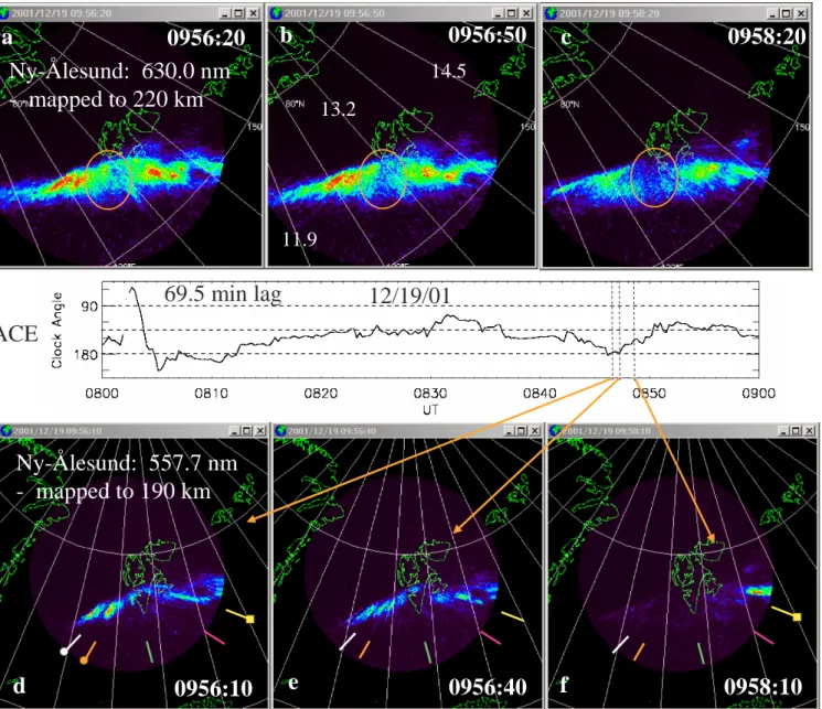
Our comparison with the IMF clock angles continues in Fig. 7 using a lag of 69.5 min. In Fig. 7a (09:54:10 UT) emissions appeared near the orange fiducial to the magnetic west of Ny- ˚Alesund while the clock angle approached 180◦. As the clock angle briefly decreased from 180◦, the emissions appeared near the green fiducial (Fig. 7b), slightly to the west of Ny- ˚Alesund’s magnetic meridian. Figures 7c and 7d illustrate emissions near the white fiducial further to the west of Ny- ˚Alesund as the clock angle returned to 180◦. In Fig. 7e the clock angle rotated back to 160◦. The

0951:20

0950:20

0952:20

0952:30

0951:00

0950:00

12/19/01

68.5 min lag

ACE

Ny-Ålesund: 557.7 nm

- mapped to 190 km

Ny-Ålesund: 630.0 nm

- mapped to 220 km

b

c

a

d

e

f

Figure 8

13.1

14.4

11.8

Fig. 8. 630.0-nm images (top) compared with the corresponding 557.7-nm images (bottom). The 557.7-nm images are the same as those in Figs. 6d, 6e, and 6f. The 630.0-nm images are in magnetic coordinates with the central meridian passing through Ny- ˚Alesund and two other meridians labeled with MLT. The orange circles in the top three images mark breaks in emissions between source regions.

clock angle reached 155◦ _{in the last image with 557.7-nm}

emissions mostly near the yellow fiducial.

Maynard et al. (2001c) suggested that the merging maxi-mizes near the edge of the high-altitude cusp at locations that depend on IMF clock angles. Figures 4–7 clearly illustrate how the locations of the 557.7-nm emissions closely follow clock angle variations. These data also show that multiple locations can be active at the same time. With clock an-gles ≤150◦, emissions came from the east of Ny- ˚Alesund. At larger clock angles source locations moved toward earlier magnetic local times. If we equate variations in the inten-sities and locations of 557.7-nm emissions with changes in rates and locations of merging on the magnetopause, we can

follow the dynamics of IMF coupling to the magnetosphere that drives ionospheric convection. In what follows we at-tempt to solidify this interpretation by relating the optical observations to other data sets, by continuing the compari-son to other intervals, and by offering a plausible cause for the emissions.

4.5 Comparisons with 630.0 nm emissions

Figure 8 compares 557.7-nm and 630.0-nm emissions from the last three intervals of Fig. 6. The 630.0-nm images are projected to 220 km and overlaid with a dipole magnetic coordinate system centered on the magnetic pole with the central longitudinal line connecting with magnetic zenith at

0956:50

0956:20

0958:20

0956:10

0956:40

0958:10

12/19/01

69.5 min lag

a

b

c

d

e

f

ACE

Ny-Ålesund: 630.0 nm

- mapped to 220 km

Ny-Ålesund: 557.7 nm

- mapped to 190 km

13.2

Figure 9

14.5

11.9

Fig. 9. Continuation of the 630.0- and 557.7-nm emission comparisons for times in Figs. 7d, 7e, and 7f. See caption for Fig. 8.

Ny- ˚Alesund. Longitudinal lines are marked every 10◦ _and

are labeled with magnetic local time. Emissions detected af-ter 13:00 MLT would be categorized as category 5 or 7 in the classification of Sandholt et al. (1998). Figure 9 displays 630.0- and 557.7-nm images for the last three intervals of Fig. 7. The emissions before 13:00 MLT in Figs. 9a, 9b, 9d, and 9e would be classified category 1. In all the 630.0-nm images in Figs. 8 and 9 there appears to be a change in char-acter just to the west of the Ny- ˚Alesund magnetic meridian near 13:00 MLT. Orange circles highlight this feature. Fig-ures 8b, 8c and 9c show distinct separations or bifurcations of the regions. The region to the east of Ny- ˚Alesund ex-tends to lower magnetic latitudes and in general has stronger emissions. This characteristic is modified in Figs. 9a and 9b, illustrating the interval when the IMF clock-angle was near

180◦_{. In Fig. 9a, a bifurcation is not obvious. However,}

emis-sions at both wavelengths, from west of Ny- ˚Alesund, are at higher latitudes than those from the east. Note that the de-tailed structuring of 557.7-nm emissions are less evident in the 630.0-nm images. This reflects a spatial smearing due to the long lifetime of the O(1D) state. As anticipated, the 630.0-nm emissions extend in magnetic local time over much more of the cusp region. We clearly associate the 557.7-nm emissions with the cusp derived from 630.0-nm observations (e.g. Sandholt et al., 1998). However, the tie to merging as the direct source observations of 557.7-nm emissions from east of 13:00 MLT places the cusp morphology in a new light. We return to this point in the discussion below.

Ny-Ålesund 630.0 nm

Ny-Ålesund 557.7 nm

Hankasalmi

Dec.19, 2001: 0952

Pykkvibaer

Hankasalmi

a

b

c

d

e

f

g

Figure 10

Fig. 10. Comparison of SuperDARN and optical data for the 2-min interval starting at 09:52 UT showing the line-of-sight velocities from

(a) Pykkvibaer, Iceland, and (b) Hankasalmi, Finland, and the spectral widths (c) of the Hankasalmi signals. The Hankasalmi spectral-width boundary has been determined and overlaid on the velocity plots. It appears in two segments because of the significant differences in magnetic latitude and the region of near null velocities in the break. The orange circle straddles the break and is at the same place as in the 630.0 nm optical data of Figs. 8 and 9. The red square highlights a region where in the previous several minutes there had been intense velocity toward Pykkvibaer. 557.7-nm all sky images are projected to (d) 150 km and (e) 190 km and overlaid on a geographic map. To emphasize the changing 557.7-nm images, two times are presented in (e) and (f) projected to 190 km. 630.0 nm images (g) projected to 220 km are overlaid on a geomagnetic coordinate map. Magnetic local times are noted for three meridians. The spectral width boundaries are overlaid as white lines.

4.6 SuperDARN measurements

Figure 10 is a composite of the radar and optical data for the two-minute period starting at 09:52 UT. Figures 10a and 10b show the line of sight velocity distributions detected at Pykkvibaer and Hankasalmi, respectively. Figure 10c plots the spectral width determined by the Hankasalmi radar. Fig-ures 10d, 10e, 10f and 10g depict the all-sky data on com-parable scale plots. How well the plots compare depends in part on the accuracy of our assumptions about the altitudes of the source data. The 557.7-nm emissions are projected to altitudes of both 150 and 190-km to capture the range of optical responses due to differences in energies of source electrons. Figures 10e and 10f show the 190 km projections of the 557.7-nm data at 09:52:30 and 09:53:30 UT to illus-trate the variability of the local dynamics during the 2-min radar scan. The 630.0-nm data were projected to 220 km and are displayed in MLat-MLT coordinates. The MLT of three meridians at the times of observations are noted. Our best estimate of the boundary between regions of high and low

spectral width as determined in Fig. 10c, is overlaid on the other panels (as white lines on the all-sky figures). Note that the spectral-width boundary is split into two parts, reflecting toward and away bifurcations of ion drift measurements and a region where echoes are weak to non-existent. The split occurs in the region where the optical properties of 630.0 nm emissions change, as marked by orange circles in Figs. 8 and 9, as well as in Fig. 10. The bifurcation between the east and west branches is striking in Fig. 10b.

The SuperDARN boundaries match the equatorward boundary of optical emissions quite well. The plasma ve-locity observed at Hankasalmi is toward the radar on the east side of the pattern and away on the west. This is consistent with the dusk-dawn flow in the cusp expected under positive BY IMF conditions. At Pykkvibaer in the region straddling

the western boundary segment (red box) the flow is mixed. Two minutes earlier the flow in that region was strongly westward. Strong away flow also straddles this boundary in this region at Hankasalmi. The flow components from both radars combine to indicate a dusk-dawn flow or a poleward

Hankasalmi

Pykkvibaer

Ny-Ålesund 630.0 nm

Ny-Ålesund 557.7 nm

Dec.19, 2001: 0954

Hankasalmi

a

d

e

f

g

b

c

Figure 11

flow. These directions are expected poleward of the open-closed boundary, but not equatorward of it. The conclusion would be that the derived boundary is probably poleward of its actual location. Chisham et al. (2002a, b) suggested that a poleward displacement of the spectral width boundary should be expected when merging proceeds in the opposite hemisphere. A longer transmission time results for energy to traverse to the observational site and heat the plasma, during which the field lines have been convected poleward and west-ward. Even subsolar merging would provide some poleward displacement compared to merging near the local hemisphere cusp. Only ground scatter is observed by the Pykkvibaer radar from the region over Ny- ˚Alesund. This is typical of the data on this day.

Scans beginning at 09:54 UT are given in Fig. 11. DMSP F13 entered the radar fields of view during this period. Its po-sition at the start of the scan is marked by the small orange-filled circle. The approximate position where DMSP later crossed the open-closed boundary is indicated by an open circle near the east coast of Greenland. The interval includes the onset of 557.7 nm emissions from west of Ny- ˚Alesund, which we identified with the IMF clock angles’ switch to ∼180◦. Six hundred and thirty-nm emissions are also more intense in this region. A comparison of images of Figs. 11e and 11f show that 557.7-nm emissions intensified during the sweep. Note that plasma flow recorded by Pykkvibaer near the west spectral-width boundary has switched back to

strongly westward (blue), as it was at and prior to 09:52 UT. Plasma flows away from Hankasalmi remained very strong in the western beams, consistent with the spatial distribu-tion observed by the DMSP F13 drift meter. The 557.7- nm emissions continued to be strongest near the spectral width boundaries. Again, the spectral width boundaries and the Hankasalmi flows are split in the region highlighted by the large orange circle.

Our comparison of radar and optical measurements at these and other times confirms the validity of using Super-DARN spectral-width boundaries as proxies for the open-closed field line boundary. It coincides with the location of the 557.7-nm emissions which we are associating with active merging. For the most part, it is also near the equatorward edge of the 630.0-nm emissions, at least in the eastern seg-ment of the boundary. While the emissions just to the west of Ny- ˚Alesund came from locations close to the boundary, those coming from still further to the west tended to be pole-ward of the spectral-width boundary. The western segment of the spectral-width boundary was poleward of the eastern segment, especially when the clock angle was smaller, em-phasizing that the source region for each is different, proba-bly with longer transit times to the western source (Chisham et al., 2002). Note that the latitude difference between the western and eastern segments is less in Fig. 11, which repre-sents the interval when the clock angle was near 180◦. That the source regions differ is consistent with both the gap or

12.5 13.8 11.2 12.5 11.2 13.8

ACE

0909:30

_0910:30

0911:50

0914:00

0914:20

0911:30

557.7 nm;

190 km

557.7 nm;

190 km

557.7 nm;

190 km

557.7 nm;

190 km

630.7 nm;

220 km

630.7 nm;

220 km

a

_b

c

d

e

f

Figure 12

orange arrows, using a 71-min lag. (a), (b), (d), and (e) present 557.7-nm emissions. (c) and (f) present the nearest 630.0-nm images to the times of (d) and (e). The orange circles in (c) and (f) highlight a bifurcation in the emissions and are located at the same MLT as the orange circles in the previous figures. The yellow circles indicate a new change in character of the 630.0 nm emissions that is not visible in the all-sky field of view at the later times presented in previous figures.

bifurcation of 630.0-nm emissions and with the plasma ve-locity measurements just west of Svalbard, as seen by the Hankasalmi radar (compare Figs. 8–11).

4.7 Earlier time intervals

If this association of the 557.7-nm emissions with the IMF is robust, we should be able to associate other time inter-vals in the same way. A 15-min interval, 25 min after lo-cal magnetic noon, is explored in Fig. 12. This 09:10 to 09:15 UT period is one of enhanced emissions in both 557.7 and 630.0 nm as seen in the meridian scan data of Fig. 3. It was found that a longer lag of 71 min was needed, consis-tent with the variable lag displayed in Fig. 1. The 557.7-nm

images for four times are displayed in Figs. 12a, 12b, 12d, and 12e. Figures 12c and 12f display the closest 630.0-nm image to those in Figs. 12d and 12e. The ACE clock angle was near 160◦until it abruptly shifted to less than 90◦. Note that while Cluster also saw a decrease in BZ, it did not

re-verse, indicating that the clock angle stayed greater than 90◦ (Fig. 1d). Figures 12e and 12f correspond to the change in clock angle. The emission pattern in Fig. 12e shifted east-ward relative to that found in the previous 557.7-nm images, as anticipated from the smaller clock angle. Figures 12c and 12f show strong emissions in the center of the band. The region to the east is also enhanced in Fig. 12f. The orange circle in each highlights a break in the emissions. This is located at the same local time, ∼13:00 MLT, as the break

in the emissions (Figs. 8a–8c and 9a–9c) and in the spectral width boundary seen later near 09:50 UT. There is a second place where the character of the 630.0 nm emissions change, which is just before magnetic noon and highlighted in Fig. 12 by the yellow circles. This region would be out of the opti-cal field of view in Figs. 8d–8f. The F13 DMSP potentials measured later in UT suggest that the tip of the morning con-vection cell should be associated with the emissions to the west of this second break. The strong emissions in between the yellow and orange circles appear at a time when the clock angle is of the order of 160◦. Of importance here is the ob-servation that the 557.7-nm emission locations change with clock angle and are continually varying with time and loca-tion, similar to the behavior observed near 09:50 UT, and to that anticipated from the conceptual picture of source regions of Maynard et al. (2001c). We return to these points in our discussion of possible source configurations.

4.8 Polar observations of keV electrons associated with merging

The previous sections established a plausible dependence of 557.7-nm variability on changes in the IMF clock angle. We next develop a rationale for interpreting these variations as signatures of merging based on Polar observations of en-hanced electron fluxes conjugate to active merging sites on the magnetopause. Unfortunately, Polar’s orbital plane is far from the dayside magnetopause and active merging sites in December, when optical images of cusp dynamics may be acquired at Ny- ˚Alesund. This association must be made in-directly. We begin by noting that precipitating electrons with energies (E) of ∼500 eV stop at altitudes near 190 km (Rees, 1963). Higher energy electrons penetrate deeper; 1 keV elec-trons lose most of their energy near 150 km. Excitation of the 557.7-nm atomic oxygen line falls off at higher altitudes because of decreased neutral density. Significant 557.7-nm emissions, therefore, require electron fluxes with E≥0.5 keV. Magnetic merging at the magnetopause breaks electron gyrotropy and changes the pitch angle distribution of trapped plasma sheet electrons, creating a field-aligned high-energy tail in the distribution at energies >0.5 keV. Maynard et al. (2003b) identified a number of merging events during Po-lar crossings of the dayside magnetopause, from signatures of accelerated ions, wave Poynting flux and, in some cases, successful Wal´en tests. In many cases merging occurred at high latitudes. Figure 13 presents data acquired during a sequence of magnetopause crossings on 1 April 2001. Fi-gure 14a shows the field-aligned component of wave Poynt-ing flux (1E×1B/µ0), consistent with Alfv´en waves

car-rying electromagnetic energy and field-aligned current away from merging sites (Maynard et al., 2003b). Figures 13b, 13c, and 13d show the total electron number density, the in-tegral number density above 300 eV and the inin-tegral elec-tron number density above 1 keV, respectively. Figure 13e shows the Z component of measured magnetic fields. In this case magnetopause crossings are identified by transitions from northward (red) to southward (blue) magnetic polarity.

Figure 15 a b c d e f g h i j April 1, 2001 n ( cm -3) n ( cm -3) n ( cm -3)

Fig. 13. Polar data acquired during three magnetopause crossings on 1 April 2001. From top to bottom the panels show (a) paral-lel Poynting flux, (b) electron number density, (c) number density of electrons with energies >300 eV, (d) electron number density with energies above 1 keV, (e) northward component of the mag-netic field measured at Polar, (f) and (g) spectrograms showing electrons with energies >500 eV and the fluxes over the whole in-strument range, (h), (i), and (j) ion spectrograms showing the paral-lel, perpendicular and antiparallel fluxes. Accelerated ions, parallel Poynting flux and a high-energy tail on the electron distributions are seen on both sides of the magnetic field reversal in the central crossing. KeV electrons are seen on the magnetosphere side, espe-cially at the other two magnetopause crossings. Poynting flux is not calculated because of the lack of knowledge concerning the correct background level for B in the presence of the field reversal. Vertical lines highlight the correlation between the electron peaks, Poynting flux and accelerated ions.

The bottom half of Fig. 13 shows differential fluxes of electrons (Figs. 15f, 15g) and ions parallel (Fig. 13h), per-pendicular (Fig. 13i) and antiparallel (Fig. 13j) to the mag-netic field, measured by HYDRA and presented in energy-versus-time spectrogram formats. Attention is directed to detections of an enhanced high-energy tail in electron fluxes, which are coincident with accelerated ions and wave Poynt-ing flux durPoynt-ing each magnetopause crossPoynt-ing. In particular, enhanced parallel ion fluxes (Fig. 13h) and wave Poynting vectors (Fig. 13a) propagated from latitudes below the space-craft near 05:30 UT, corresponding to a clock angle near

-200 0 200 δ B Y ( n T ) δ B Z ( n T ) -200 0 200 400 -400 December 19, 2001 557.7 nm image times Figure 14 a b c d e

Fig. 14. High resolution DMSP F15 data showing two components of the perturbation magnetic field, electron and ion spectrograms, and the vertical and horizontal drifts. The negative slope of the per-turbation magnetic fields indicates upward Region 1 currents. The colored circles denote the central times of 557.7-nm images pre-sented in Fig. 15. Note that the first three correspond to electron en-hancements, as well as intensification in the field-aligned currents (steeper slope) from the magnetometer records denoted by the ver-tical dashed lines.

160◦(Maynard et al., 2003b, Table 1). The high-energy tails of electron distributions (Figs. 13c, 13d, and 13f) are also structured. Vertical dashed lines show that each spike in the high-energy electrons lines up with parallel Poynting flux for this crossing. Similar enhancements of high energy electrons are seen at the other two crossings where principal parallel ion fluxes are from above the spacecraft and the clock angle is near 130◦. Note that if enhanced high-energy fluxes had tracked the total number flux (Fig. 13b), this would have in-dicated electron heating or just an increase in density rather than a change in the distribution. However, the enhancements are strongest and deviate most significantly from the inte-gral number flux near magnetopause crossings. While quasi-neutrality requires that the bulk of the electron populations must travel with the ions, electrons in the high-energy tail can move ahead and reach the ionosphere before the main popu-lation. We expect to see these electrons first near the open-closed boundary, at footprints of field lines recently opened (Scudder et al., 1984).

Polar measurements provide evidence that electrons with sufficient energies to excite 557.7-nm emissions are a normal consequence of active merging. The skimming nature of Po-lar’s orbit favors interpreting the enhancements observed in the high-energy electron fluxes as reflecting temporal

varia-the 557.7-nm emission time constant is ∼1 s, temporal vari-ations in emissions should reflect temporal varivari-ations in the source. Away from active merging sites fluxes of electrons with E>0.5 keV is diminished. These facts support our use of 557.7-nm intensifications as proxies for active merging. To test this association, we return to the F15 measurements above Ny- ˚Alesund.

4.9 DMSP electron observations associated with 557.7-nm emissions

DMSP F15 passed close to the afternoon open-closed bound-ary to the southeast of Ny- ˚Alesund. Near 09:24 UT it en-countered precipitating electrons in the vicinity of the ob-served optical emissions. Figure 14 shows an expanded plot of F15 measurements from this interval. Figures 14a and 14b show δB variations in the spacecraft-centered Y and Z coordinates (see Sect. 2). Between 09:24:00 and 09:24:24 1BY and 1BZdecreased from −38 and −61 nT to minima

of −209 and −301 nT, respectively. The region of nega-tive slopes corresponds to a current out of the ionosphere, largely carried by precipitating electrons. The correlated changes in δBY and δBZof 171 and 240 nT indicate that F15

crossed a FAC sheet at an attack angle of about 55◦. The total magnetic perturbation in the sheet was 295 nT, which corresponds to J|| of ∼0.23 A/m. The average current

den-sity out of the ionosphere was about 1.6 µA/m2. In cross-ing the sheet the average integrated number flux of down coming electrons with energies between 30 eV and 30 keV was ∼109/cm2-s-sr. Assuming a moderately field-aligned pitch angle distribution, the electron flux measured by J4 on F15 accounts for the 1.6 µA/m2_{current density inferred from} SSM measurements. Vertical dashed lines highlight parallel current maxima and tie these enhancements to the increases in the electron fluxes.

Color-coded dots shown at the top of the electron spec-trogram denote the center times of the 5-s-interval of each 557.7-nm images shown in Fig. 15. The positions of F15 mapped along the magnetic field to 190 km are indicated by the color-coded dots. The 557.7-nm images have been mapped to 190 km as before. To better illustrate correspon-dence between 557.7-nm emissions and precipitating elec-trons the range of all-sky images were extended from zenith angles of 75◦_{to 80}◦_{. Comparison of Figs. 14 and 15c–15e}

reveal that the electron bursts observed between 09:24:00 and 09:24:30 UT match enhancements of 557.7-nm emis-sions. Some individual electron spectra in this region have “inverted V” signatures characteristic of field-aligned accel-eration above the ionosphere. This accelaccel-eration is in addi-tion to energies indicated by Polar as due to merging. We find that spectra outside of the “inverted V” structures have high-energy tail distributions similar to those observed by Polar when conjugate to merging sites on the magnetopause. Thus, the electron fluxes measured by DMSP appear to be the source of the 557.7-nm emissions.

557.7 nm

190 km

Z80

Hankasalmi

a

b

c

d

e

f

12/19/01

0924 UT

Figure 15

Fig. 15. (b − f) 557.7-nm all-sky images. The images have been extended to 80◦zenith angle to cover the mapped positions of DMSP (color-coded circles). Note that in both (c) and (d) the mapped position of DMSP coincides with the optical emissions. SuperDARN line-of-sight velocities from Hankasalmi are displayed in (a), along with the DMSP positions for three times. The large horizontal drift observed by DMSP near 09:24:30 UT is in a region apparently dominated by ground scatter observations.

Plasma velocities measured by the SuperDARN radar at Hankasalmi are shown in Fig. 15a for the interval starting at 09:24 UT. Mapped positions of DMSP at three times are overlaid on the velocity data. No significant velocities were detected by SuperDARN near the mapped DMSP locations. A strong burst of antisunward flow was observed by DMSP F15 co-located with the equatorward edge of these enhanced electron fluxes (Fig. 14e). A comparison of data in Figs. 14e with 14a and 14b shows that the large flow region is pri-marily in the downward current region. We also checked the RPA measurements of the in-track component of plasma drift. Significant along-track flows are seen. However, their magnitudes and variability are not trustworthy because of the effects of small changes in the spacecraft potential on the analysis of the RPA current-voltage sweeps. The antisun-ward flows perpendicular to the orbit track, combined with probable flow along the orbit track, suggest that the resulting plasma velocity vector was nearly at quadrature to the Super-DARN line-of-sight. This may explain why the radar did not observe flows in that region. A second, and more probable, possibility is that real signals were obscured by ground

scat-ter in this region. Finally, we note that similar large ampli-tude electric fields were observed by DE-2 at the open-closed boundary (Maynard, 1985; Maynard et al., 1991), and strong westward ion drifts in the cusp are associated with merging when BY is positive (Maynard et al., 2003a).

5 Discussion

We have shown that temporal and spatial variations in all-sky images of 557.7-nm emissions are related to variations in the IMF clock angle. The spatial position is qualitatively consis-tent with the conceptual diagram of Maynard et al. (2001c), in which merging occurs around the rim of the high-latitude cusp at positions dependent on the IMF clock angle. We re-lated the 557.7-nm emissions to a historical picture of the cusp based on 630.0-nm emission morphology, as well as SuperDARN and DMSP observations. Polar measurements show that high-energy electrons (≥0.5 keV) are emitted from active merging sites. This observation provides a plausible source for electrons responsible for the green line emissions