HAL Id: hal-01342465
https://hal.inria.fr/hal-01342465v2
Submitted on 25 May 2017
HAL is a multi-disciplinary open access
archive for the deposit and dissemination of
sci-entific research documents, whether they are
pub-lished or not. The documents may come from
teaching and research institutions in France or
abroad, or from public or private research centers.
L’archive ouverte pluridisciplinaire HAL, est
destinée au dépôt et à la diffusion de documents
scientifiques de niveau recherche, publiés ou non,
émanant des établissements d’enseignement et de
recherche français ou étrangers, des laboratoires
publics ou privés.
Surfacing Curve Networks with Normal Control
Tibor Stanko, Stefanie Hahmann, Georges-Pierre Bonneau, Nathalie
Saguin-Sprynski
To cite this version:
Tibor Stanko, Stefanie Hahmann, Georges-Pierre Bonneau, Nathalie Saguin-Sprynski.
Surfac-ing Curve Networks with Normal Control. Computers and Graphics, Elsevier, 2016, 60, pp.1-8.
�10.1016/j.cag.2016.07.001�. �hal-01342465v2�
Surfacing Curve Networks with Normal Control
Tibor Stankoa,b,c, Stefanie Hahmannb,c, Georges-Pierre Bonneaub,c, Nathalie Saguin-Sprynskia,b
aCEA, LETI, MINATEC Campus, Grenoble bUniversit´e Grenoble Alpes cCNRS(Laboratoire Jean Kuntzmann), Inria
Abstract
Recent surface acquisition technologies based on microsensors produce three-space tangential curve data which can be transformed into a network of space curves with surface normals. This paper addresses the problem of surfacing an arbitrary closed 3D curve network with given surface normals. Thanks to the normal vector input, the patch finding problem can be solved unambiguously and an initial piecewise smooth triangle mesh is computed. The input normals are propagated throughout the mesh. Together with the initial mesh, the propagated normals are used to compute mean curvature vectors. We then compute the final mesh as the solution of a new variational optimization method based on the mean curvature vectors. The intuition behind this original approach is to guide the standard Laplacian-based variational methods by the curvature information extracted from the input normals. The normal input increases shape fidelity and allows to achieve globally smooth and visually pleasing shapes.
Keywords: shape reconstruction, curve network, normal input, smooth surface
1. Introduction
Traditionally, digital models of real-life shapes are ac-quired with 3D scanners, providing point clouds for sur-face reconstruction algorithms. However, there are situ-ations when 3D scanners fall short, e.g. in hostile envi-ronments, for very large or deforming objects. In the last decade, alternative approaches to shape acquisition using data from microsensors have been developed [1,2]. Small size and cost of these sensors facilitate their integration in numerous manufacturing areas; the sensors are used to obtain information about the equipped material, such as spatial data or deformation behavior. Ribbon-like devices
incorporated into soft materials [3] or instrumented
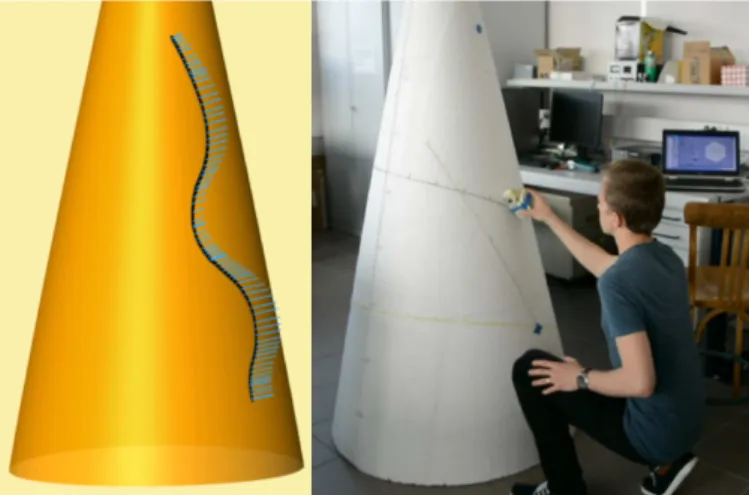
mo-bile devices moving on the surface of an object provide tangential and positional data along geodesic curves – see Figure2for an example acquisition setup. In this context, we focus on the resulting problem of surface reconstruc-tion and leave aside all issues related to acquisireconstruc-tion and transformation of sensor signals into geometric data.
We address the problem of fitting a smooth surface to given discrete positional and normal data along a net-work of 3D curves. The goal is to obtain a fully auto-matic, efficient and robust method producing fair and vi-sual pleasing surfaces consistent with the shape suggested by the input curves. A common practice in shape mod-eling is to rely on normal vector input in order to en-hance shape quality and fidelity. Normal input can be found e.g. as boundary constraints in variational modeling [4,5,6], as geometric invariants [7], for computing flow-fields guiding the surface construction process, as Hermite data in surface fitting [8,9] or indirectly describing
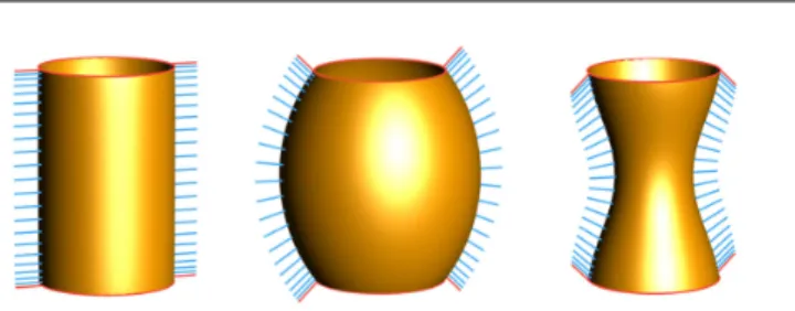
silhou-Figure 1: Influence of input normals: the two circular curves (red) are given as input together with normal vectors of different orientation (red normals). Propagation of the input normals over the surface (blue) guides the computation of three different shapes.
ette constraints [10,11] or shading behavior of 2D and 3D shapes [12,13,14] to cite a few possible applications.
More generally, surfacing 3D networks is a fundamen-tal problem in geometric modeling. Apart from traditional CAD modeling [15,8,16,9], sketch-based interfaces [17,
18,19] and sketch-based modeling techniques [20,21,22,
23,24,25] have recently become increasingly popular in a range of versatile application areas. Even though normal vectors are not part of a typical sketch-based modeler out-put [26,17,18], recent state of the art [24] in surfacing 3D curve networks however requires estimation of normal vectors along the curve network.
The method we propose is a new mesh-based data-driven variational approach. We show how to generate high quality surfaces faithful to the input data by solving linear systems only. The key insight is the decoupling of normals from positions for the curve-to-patch extrapola-tion. The method first interpolates positions and normals separately over patches enclosing cycles of curves, then
Figure 2: In this example, we scan curves with normals on the cone using the Morphorider, a small mouse-like device instrumented with microsensors. The position and normal information along the scanned curves can serve as input to our algorithm.
estimates mean curvature values at vertices, and finally optimizes for positions that best match the mean curva-ture vector formed by the mean curvacurva-ture value and nor-mal computed in the previous steps. The combination of shape and normal optimization into a compact expression has the advantage of not requiring the usual reformulation of normal constraints into layers of positional boundary constraints.
Contributions. This paper is an extended version of the earlier short paper [27] in which we have first introduced a variational approach for smooth surface modeling to fit a given curve network with surface normals. The main contribution of the earlier short paper was to combine the standard Laplacian with a term based on estimation of the mean curvature normal. The intuition behind this original approach was to guide the standard Laplacian-based vari-ational methods by the curvature information extracted from input normals. The normal input increases shape fi-delity and allows to achieve globally smooth and visually pleasing shapes.
In comparison with the original short paper, this pa-per provides an expanded discussion of a modified mean curvature estimation used inside our Laplacian-based sur-face modeling framework that supports the generation of a continuously varying normal vector field. Our mean curvature estimation blends the positional and normal in-put so that the solution of our optimization conforms to both constraints. Additionally, we propose a simplified and more compact version of the energy functional used to compute a globally smooth surface with constraints along curve network. Most importantly, we provide more re-sults, a convergence analysis and an in-depth comparison of our algorithm with state of the art methods.
2. Related work
Surfacing curve networks. With the advent of sketch-based modeling tools, such as interactive 3D sketching tools [26,
28,17,18] or methods inferring 3D curve networks from
2D sketches [29, 19], considerable effort has been
ded-icated to the design of methods for surfacing curve net-works originating from sketching tools [20, 30, 31, 32,
24]. The common assumption in these works is that the
underlying curve network was created with some design intent, and that the input information is minimal. Rose
et al. [20] solve the patch finding problem and compute
a developable boundary triangulation. Bessmeltsev et al.
[31] interpolate a general 3D network of curve cycles by
computing quad-mesh patches whose isolines capture the design flow inherent in the network. Sadri and Singh [32] compute self-intersection-free surface patches based on a flow complex induced by the boundary curves. Both methods compute surface patches individually and do not seek a globally smooth surface across dedicated boundary
curves as we do. Pan et al. [24] use rotation-minimizing
frames along the curves to estimate normal vector input and construct globally smooth surface patches having a curvature direction field consistent with an orthogonal flow field implied by the boundary curves. This makes sense in the setting of sketch-based modeling where the artist-drawn input represents particular characteristic shape cur-ves, such as representative flow-lines. This is a strong as-sumption on the input network we do not make; our input curves, in contrast, can have arbitrary shapes (Figure9). n-sided patches. n-sided boundary patches – possibly with prescribed tangent ribbons to achieve G1-continuity across
boundary curves – can be computed using transfinite
inter-polation methods (Coons patches [15], Gregory patches
[8], Generalized B´ezier patches [9] or subdivision
approa-ches [33]). The first group of methods assumes a
pre-segmentation of each input cycle into n curve segments with low-distortion mapping to a convex planar n-sided polygon. Prescribed tangent ribbons must be defined con-sistently and twists estimated accordingly. Methods in the second group quadrangulate the input cycles with topo-logical guarantees on the extraordinary vertices and ap-proximate the coarse mesh using well-known subdivision schemes. The variational approach of Boier-Martin et al. [34] integrates normal constraints by locally fitting the vertex neighborhood with a quadratic polynomial in order to estimate partial derivatives. However, the integration of normal constraints violates the independence of spatial dimensions of the linear system to solve.
Shading-based variational modeling. Gingold and Zorin [12] modify a given input shape by drawing strokes on a shaded image of the surface. The strokes indirectly impose nor-mal constraints that are solved by modifying the position of the surface along the strokes, while the normals of the surface outside the strokes should not change. In contrast, 2
we impose both positional and normal constraints along input curves, and compute new positions and normals ev-erywhere else.
Variational modeling with normal constraints. The mini-mum variation surfaces [35] enable direct prescription of normals and principal curvatures along a curve network and may result in high quality shapes; however, the result-ing optimization is nonlinear. Thanks to their speed and robustness, linear variational surface modeling and defor-mation methods have attracted an impressive amount of interest in the past few years, even though they only pro-vide approximate results with respect to nonlinear
prob-lems; see the survey by Botsch and Sorkine [36]. We
focus on linear methods using normal constraints in ad-dition to standard positional constraints. The boundary
constraint modeling methods of Botsch and Kobbelt [4],
Jacobson et al. [5], and Andrews et al. [6] prescribe Ck
continuity indirectly either by fixing k − 1 rings of vertices or by adding a ghost geometry. Setting additional rings of vertices consistently with Ckcontinuity at intersections
of constrained curves is not a trivial task. This issue, re-ferred to as twist compatibility problem or vertex
consis-tency problem [37], arises when joining smooth patches
around a common vertex of arbitrary valence with tangent plane continuity. Jacobson et al. [5] solve the problem by freezing the 1-neighborhood of each vertex with normal constraint. Vertices with conflicting neighborhoods are fixed in the least-squares sense. Andrews et al. [6] propose a linear variational modeling system from curve networks using a ghost geometry for solving inconsistent Laplacian constraints. This technique only enables to generate sharp
edges along arbitrary curves. Schneider and Kobbelt [38]
propose a multigrid fairing method with prescribed posi-tions and normals; only constraints along simple curves are considered. Crane et al. [39] present a fairing method using Willmore flow expressed in curvature space that al-lows to prescribe positions and binormal vectors along the surface boundary.
All these methods share the treatment of normals as boundary constraints when computing the positions. Our approach is different. By separately interpolating normals and positions before combing them into a mean curvature vector field which is then used to compute the best match-ing surface, the propagated normals serve as a guidmatch-ing vector field as illustrated in Figure1. We therefore avoid the vertex consistency problem and can deal with nor-mal constraints even at the intersection of multiple curves. More importantly, unlike all the approaches above, our method does not require an extra parameter to control the magnitude of normals.
3. Framework
The surface S we aim to reconstruct is a connected 2-manifold, with or without boundary, parameterized by
p : Ω ⊂ R2 → S ⊂ R3. Moreover, the tangent space
Tp(S)varies continuously. Next, we consider a curve
net-work C ⊂ S which is connected and closed. The curves ck(t) = p (u(t), v(t)) ∈ C are C1 smooth and without
self-intersections; the intersection of two different curves is ei-ther empty or a discrete set of points. Knowing the topol-ogy of the curve network C, the input to our algorithm is a discrete sample of positions pi= ck(ti)= p (u(ti), v(ti)) ∈ C,
together with the unit surface normals ni⊥ Tpi(S).
3.1. Overview of the method
We use the following pipeline to generate a globally smooth surface from curve and normal vector input:
1. Raw data are first interpolated with cubic splines and resampled uniformly. We efficiently detect the network cycles, then triangulate them in plane. 2. By solving two biharmonic systems with boundary
constraints, we both propagate the surface normals and obtain an initial guess for the vertex positions; this allows us to compute discrete mean curvature for the whole mesh.
3. Finally, we solve a linear optimization problem com-puting a surface that best matches the mean curva-ture vector formed by the mean curvacurva-ture value and the normal computed in the previous step.
3.2. Exploiting local tangent space to detect cycles
The detection of cycles in a general curve network is a complex and ambiguous problem, often without a unique solution. In order to overcome this problem, methods for surfacing sketched networks adopt a variety of heuristics
to mimic the human perception [30]. In our specific
set-ting, due to the assumptions on surface smoothness and manifoldness, and the availability of the oriented normals, any possible ambiguity can be efficiently resolved as fol-lows.
Let us call a node the intersection between two or more curves. A segment is a portion of curve bounded by two ad-jacent nodes. A cycle is a set of adad-jacent segments which constitute a boundary of some surface patch; the curve cy-cles are assumed to be contractible on S. Our algorithm is inspired by face extraction in edge-based data structures for manifolds. First, the segments adjacent to any node are cyclically sorted with respect to the orientation given by the input normal at that node. Then, starting from any (Node, Segment) pair, we trace a unique cycle by choos-ing the next node as the other endpoint of the current seg-ment. The next segment is then picked from the ordered set. To handle surfaces with boundary, we require the user to tag all boundary segments.
3.3. Network tessellation
We represent the surface S as a triangle mesh M =
(V, F )with vertices V and faces F . Prior to the tessella-tion, the positions piand normals ni along the curve
with arc length parameterization, providing a uniformly
sampled network (Figure 8 top). Each cycle defines a
closed 3D curveΓ bounding an n-sided surface patch. We
triangulate a planar projection of each cycle individually to obtain the topology F of the whole mesh; the
triangu-lation is computed using Shewchuk’s Triangle [40]. The
plane of projection for each cycle is defined by the aver-age position ˜p and averaver-age unit normal ˜n computed from
resampledΓ.
Even though this simple planar projection is not nec-essarily injective, we have found that it leads to a much smaller distortion between the planar triangulation and the mesh triangulation, in comparison with other planar
embeddings ofΓ with guaranteed injectivity (e.g. mapping
to a circle or a polygon). Notice that a more robust but
time-consuming 3D curve tessellation method can be used [41].
3.4. Variational smoothing
At this point of the process we have computed the topology F of the mesh M, and we have the constraints – positions and normals – for vertices along the resampled curve network C. In this section, we describe a variational method for computing the positions of the free vertices, based on the discretization of the Laplace-Beltrami opera-tor and of the mean curvature vecopera-tor for piecewise linear surfaces.
Discretization of∆. Given a piecewise-linear function fi =
f(vi)defined over the vertices vi∈ Vof M, the
discretiza-tion of the Laplace-Beltrami has the form [36] ∆ f (vi)= wi
X
j∈N1(i)
wi j( fj− fi)
where N1(i)is the index set of 1-ring neighborhood of vi.
The vertex weights are stored in the diagonal mass ma-trix Mii = 1/wi, while the edge weights wi j are stored in a
symmetric matrix Ls (Ls)i j = −P k∈N1(i)wik, i = j, wi j, j ∈ N1(i), 0, otherwise.
The discrete Laplace operator is then characterized by the matrix L= M−1L
s. In the following, we use the cotangent
Laplacian wi = 1/Ai, wi j = 21(cot αi j+ cot βi j)where αi jand
βi j are the two angles opposite to the edge (i, j), and Aiis
the Voronoi area of vi[42].
Initial vertices and propagated normals. Let Vcdenote the
set of vertices lying on the curve network C, and Vf
de-note the remaining free vertices. We start by computing initial positions and initial normals for all vertices by
solv-ing two biharmonic systems: L2V∗ = 0 for positions and
L2N∗ = 0 for normals. The propagated normals N∗ are
then normalized. We choose L as the cotangent Lapla-cian based on the planar triangulation computed in
Sec-tion3.3. The positional and normal boundary conditions
are incorporated into the systems as hard constraints by
eliminating the corresponding rows of the matrix L2 as
described in [43].
Mean curvature guide. From the initial vertices v∗and the
propagated normals n∗we now compute mean curvature
information that will guide the optimization. Following Sullivan [44], the discrete mean curvature vector at a mesh vertex v is proportional to the integral of the conormal η = n × e, i.e. the vector product of the normal and the unit tangent to the boundary,
2h(v)=
I
∂N1 η ds
computed along the boundary of the 1-neighborhood N1of
v. Sullivan [44] evaluates this integral using the triangle normals defined by the mesh vertices v.
v∗i+1 v∗ v∗i n∗i n∗i+1 n∗ h
In order to take the input data into account, we evaluate this inte-gral using the
propa-gated normals n∗ rather
than the triangle nor-mals. More precisely, we compute the mean
cur-vature vector for the initial surface by summing the con-tributions for all oriented edges opposite to v∗:
h(v∗)= 1 A n−1 X i=0 n∗+ n∗i + n∗i+1 kn∗+ n∗ i + n ∗ i+1k × (v∗i+1− v∗i), (1)
where n∗ denotes the propagated normal at the vertex v∗
of valence n, whose Voronoi area is A and its neighbors are v∗i (indices taken modulo n, see inset).
Formula (1) for computing the mean curvature is a key part to our method. Its originality lies in blending together the positional information (the initial vertices v∗) with the
additional normal information (the propagated normals n∗) not directly inferred from the positions. In contrast,
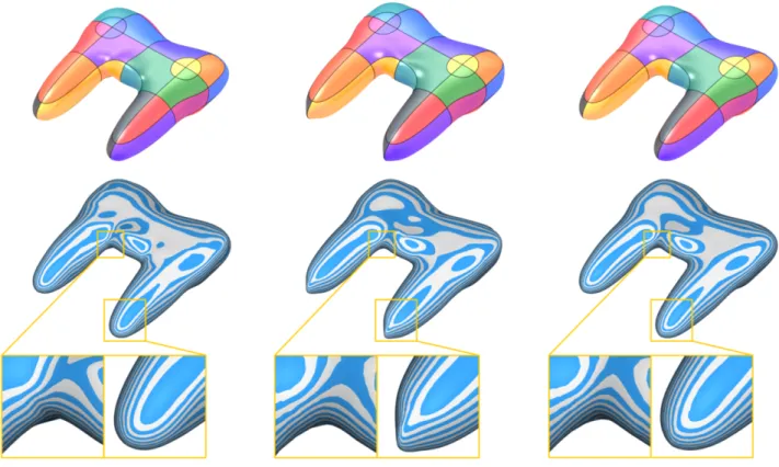
the usual discrete mean curvature formulations, such as the cotan formula [42], rely solely on vertex positions. We illustrate this originality in Figure3, where we show three
discrete mean curvatures, one based on [42] (left), and
two on our formula (1) (middle and right) computed with
the same geometry, but using two different normal fields. It can further be observed in Figure3that our mean curva-ture measure behaves at least as well as the standard mea-sures even with a low quality mesh. Since we apply the mean curvature formula in this paper to good quality tri-angulations resulting from a planar Delaunay tessellation (Section 3.3) we did not investigate the incorporation of propagated normals into more robust discrete mean cur-vature measures such as [45].
Figure 3: Mean curvature of the irregular horse mesh. (Left) the cotan formula [42] which is based solely on the mesh vertices, (middle & right) the 3-averaging formula (1), which additionally takes into account a normal at each vertex. For the middle image, the vertex normal is taken as the average of the face normals. In the rightmost example we smoothed the vertex normals before applying formula (1).
Optimization. We can now define the energy functional
E(V)=X
v∈V
k∆v + h(v)n∗k2 (2)
with h(v) = kh(v)k being the scalar mean curvature at v.
This formulation, derived from the well-known formula ∆v = −h n, enables us to match the mean curvature and the propagated normals. In order to exactly interpolate
the positional constraints Vc, we perform the following
optimization:
min E (V) s.t. v= v∗for all v ∈ Vc. (3)
The energy E is written in matrix form as E(V)= kLV − 2Hk2 and minimized by solving
"L>L C> C 0 # "V Λ # ="LV>H∗ c # with C=hIc 0i , V = "Vc Vf # ,
whereΛ is the matrix of Lagrange multipliers, Icis the c×c
identity matrix, and H is the matrix of propagated normals
N∗scaled by the mean curvature h.
4. Results
4.1. Normal control
In Figure1we demonstrate the shape control provided
by the input normals. The fixed vertex positions are sam-pled along two parallel circles from the same cylinder while prescribing three different sets of normal vectors along the circles. With the original normals (Fig. 1left), the cylin-drical surface is nicely reconstructed. Using the two other
sets of rotated normals (Fig. 1 middle, right) results in
the barrel and bottleneck surfaces, as expected intuitively. The method works well even for challenging input data, such as the networks with large normal curvature
vari-ations and high valence curve intersections in Figure 8,
or networks with large curvature variation in the tangent plane in Figure9.
4.2. Comparison with previous methods
Botsch and Kobbelt [4] state that solving for the kth
-order Laplacian while imposing boundary conditions up to Ck−1implies a non-trivial smooth solution:
∆kS(x)= 0, x ∈Ω\δ Ω;
∆jS(x)= b
j(x), x ∈δ Ω , j < k.
(4) Notice that the authors in [4] did not implement boundary constraints directly; instead, they fixed positions of k − 1
rings of vertices to prescribe Ck−1 boundary constraints.
This setting prevents dealing with arbitrary constrained curve networks without knowing the positions of k − 1 rings of vertices. It is therefore impossible to compare our method to theirs; we can however compare our method to
the analogous formulation given by (4). To this end, we
have implemented the system (4) for k= 2. To avoid fixing the positions of 1-ring vertices along constrainted curves, we directly cast the b1as equality constraints of the linear
system. See Figure5 for visual comparison of various
er-ror metrics on sphere and torus, and Table1for numerical
analysis of distance to ground truth.
The method of Pan et al. [24] is considered the state of the art in surfacing sketched curves. We find it interesting to include a comparison with this method, although the
two algorithms do not share the same input since [24] do
not know the normals a priori. The comparison with their
method on the gamepad is shown in Figure4. The normals
along the constrained curves, required by our method,
were sampled from the final surface of Pan et al. [24].
From left to right, we show the output of Pan et al. [24], the surface computed with constrained linear differential
equation method (4) with direct prescription of normals,
and our surface.
Our method combines the algorithmic simplicity with high fidelity to the reconstructed shape, and at the same time maintains the fairness of the final surface. Inter-esting details are revealed by looking at the isophotes.
On the surface of Pan et al. [24], the isophotes are of
globally poor quality, with undesirable wiggles visible at closer inspection, see the close-up to the concave region.
Figure 4: On sketched networks, the results of our algorithm are similar to the method of Pan et al. [24], which assumes the input curves capture the flow field of the underlying surface. The isophotes on our surface vary more smoothly, suggesting higher order of continuity. Left to right: the method of Pan et al. [24]; the formulation (4) (Section4.2) with direct prescription of normals; our algorithm. All three meshes have the same normals along the curve network.
While the middle surface computed with (4) seems
glob-ally smoother than the left surface, the linearization arti-facts are evident (close-up, handle). The colored render-ings of the three surfaces look similar at the first glance; notice however the improved quality of specular highlights on our gamepad compared to the left surface.
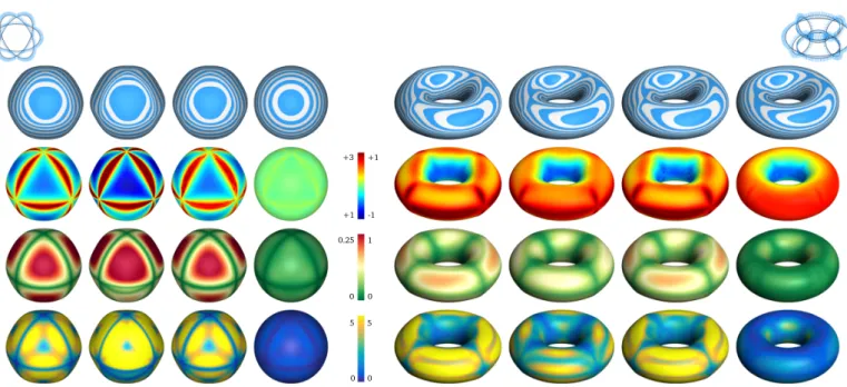
4.3. Measuring the error
In Figure5we compare three error measures on well
known geometries, the sphere and the torus: mean cur-vature, distance to ground truth and difference between propagated and computed normals. We compare the error from the standard biharmonic and triharmonic surfaces with positional constraints along the curve network (left
two columns) and the method (4) (middle right) with our
surfaces (right column). We also show the isophote pat-tern which indicates globally smooth shapes, also across the curve network.
Notice that the standard linear variational methods ex-hibit the well-known undesired defects due to the lineariza-tion of the energy funclineariza-tionals, and the shapes have high curvatures along the curve network and low curvature ev-erywhere else. In contrast our solution has a much smaller curvature variation. Many authors spend considerable ef-fort in improving the shape of linear methods using e.g. reparameterizations or multigrid methods [38, 4, 5]. It can be observed that our shapes succeed in mimicking the
data method # Vf/ Vc
distance error (Vfonly)
min max mean RMS
sphere, r= 1 ours 19545 / 738 0.0004 0.0502 0.0319 0.0343 method (4) 0.0001 0.3262 0.1412 0.1635 biharmonic 0.0006 0.2887 0.1465 0.1669 triharmonic 0.0003 0.3994 0.1641 0.1918 torus, R= 4, r = 2 ours 24321 / 564 0.0008 0.3207 0.1260 0.1464 method (4) 0.0021 0.7917 0.4095 0.4587 biharmonic 0.0028 0.7967 0.4122 0.4624 triharmonic 0.0016 0.6068 0.3255 0.3626
Table 1: Distance from analytic ground truth, measured on the free ver-tices.
desired non-linear shape behaviors simply by combining two linear processing steps: normal propagation and con-strained fitting, see the curvature plots in Figure5. We ar-gue that the normal propagation step which precomputes a continuously varying normal field is a key ingredient for this nice property.
4.4. Convergence analysis
Given an input curve network, we have computed a se-quence of initial planar triangulations (Section3.3) with a sampling distance divided by two, resulting in a num-ber of triangles approximately multiplied by four. We then
applied our variational smoothing method (Section3.4).
This process results in a sequence of meshes Mi. Since
there is no analytic form of limi→∞Mi, we illustrate the
0.25 +3 +1 +1 -1 0 1 0 5 0 5 0
Figure 5: Various error measures on the unit sphere and the torus with radii 4 and 2. Top to bottom: isophotes, mean curvature, distance from ground truth (Table1), difference between propagated and computed normals (in degrees). Left to right: biharmonic surface∆2 = 0, triharmonic surface
∆3= 0, method (4), our algorithm.
d/2 d/4 d/8 d/16 d/32 2.05E-05 1.67E-04 3.64E-05 1.91E-02 8.92E-03 7.79E-03 3.36E-03 2.07E-03 2.34E-03 7.62E-04 4.71E-04 6.18E-04 4.16E-05 1.26E-04 2.58E-04 sampling distance Hausdorff distance to the previous level : RMS sphere : d=1.44E-01 bumpy cube : d=1.33E-01 beetle : d=8.86E-02
Figure 6: The meshes computed using our method converge towards a limit surface upon refinement of the sampling distance; see Section4.4 for details.
convergence in Figure6by plotting the Hausdorff distance
between the consecutive meshes Mi, Mi+1. The three curves
correspond to the sphere (Fig.5), the beetle and the bumpy cube (Fig.8) networks.
4.5. Hard constraints vs. soft constraints
Until now, in all of our examples, the positions of all vertices along input curves were exactly interpolated as hard constraints by solving (3). In case of noisy input data, which usually occurs when acquiring data with scanning
or mobile devices (see Section 1), it might be useful to
modify the problem (3) in order to incorporate soft posi-tional constraints as follows:
Eso f t(V)= X v∈V k∆v + 2h(v)n∗k2+ ω X vs∈Vs kvs− v∗sk 2
where the constrained vertices Vcare further partitioned
into hard constraints Vhand soft constraints Vs. Figure7
illustrates the robustness of this approach; in this test, we artificially perturbed the positions and normal directions along the input network. Our method with soft constraints produces stable output, while still preserving the shape fidelity.
Figure 7: If the input data are noisy, soft constraints (right) produce better results than hard constraints (left) while still maintaining high overall shape fidelity. In this example, we artificially added 5% of noise to both positions and normals.
5. Limitations
A weakness of our method lies in the fact that the cotangent weights for the Laplacian matrix L are inferred from the planar triangulation, computed for each patch
in-dividually as explained in Section3.4. Such
parametriza-tion is not isometric to the actual surface patch; as a con-sequence, the weights are not optimal. Nevertheless our examples show that it does not impact the smoothness of our results across surface patches.
The framework cannot automatically handle curve net-works which are open or consist of more than one compo-nent. However, the optimization (3) is not limited by the
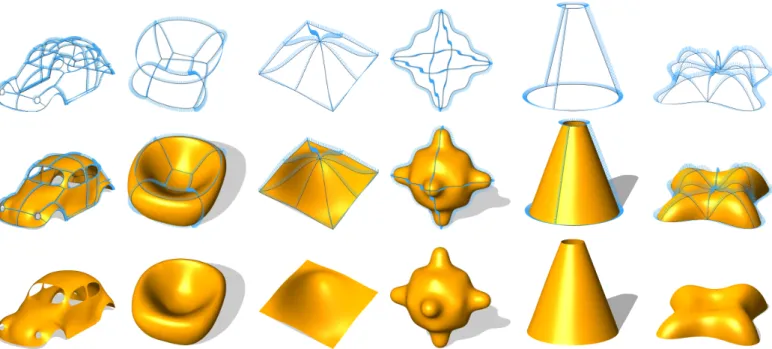
Figure 8: Smooth surfaces reconstructed using our method.
topology of the network, only by the availability of the initial mesh.
6. Conclusion
We have introduced a Laplacian-based surface recon-struction method from curve and normal input. After prop-agating the input normals smoothly over the surface and computing the corresponding mean curvature vectors, the normal constraints are integrated into the energy func-tional. Efficiency and robustness are achieved by using a linearized objective functional, such that the global op-timization amounts to solving a sparse linear system of equations.
The presented framework is intended to serve for curve networks with normal vectors acquired by mobile devices equipped with microsensors. For this application we plan the following extensions. The method, currently requiring a closed curve network, could be modified to work with open curve networks. The initial tessellation could be im-proved by using a more advanced 3D patching algorithm. Since our current implementation runs at interactive time rates (order of 0.1s for a mesh with 10k vertices and 1k constraints), we plan to allow the user to scan shapes in-teractively by incrementally adding curves. We therefore want to investigate how to update the optimization when the input data changes locally.
Acknowledgment. The meshes used in our tests were kindly
provided by Pan et al. [24] (gamepad), Leif Kobbelt (bee-tle), Cindy Grimm1(bowl), and libigl2(lilium, bumpy cube).
1
http://web.engr.oregonstate.edu/~grimmc/
2http://libigl.github.io/libigl/
References
[1] Sprynski N, David D, Lacolle B, Biard L. Curve Reconstruction via a Ribbon of Sensors. In: 14th IEEE Int. Conf. on Electronics, Circuits and Systems. 2007, p. 407–10.
[2] Hoshi T, Shinoda H. 3D Shape Measuring Sheet Utilizing Gravi-tational and Geomagnetic Fields. In: SICE Annual Conf. 2008, p. 915–20.
[3] Saguin-Sprynski N, Jouanet L, Lacolle B, Biard L. Surfaces Recon-struction Via Inertial Sensors for Monitoring. In: 7th European Workshop on Structural Health Monitoring. 2014, p. 702–9. [4] Botsch M, Kobbelt L. An Intuitive Framework for Real-time
Freeform Modeling. ACM Trans Graph (Proc SIGGRAPH)
2004;23(3):630–4.
[5] Jacobson A, Tosun E, Sorkine O, Zorin D. Mixed Finite Elements for Variational Surface Modeling. Computer Graphics Forum (Proc SGP) 2010;29(5):1565–74.
[6] Andrews J, Joshi P, Carr N. A Linear Variational System for Mod-elling From Curves. Computer Graph Forum 2011;30(6):1850–61. [7] Huard M, Sprynski N, Szafran N, Biard L. Reconstruction of Quasi Developable Surfaces from Ribbon Curves. Numerical Algorithms 2013;63(3):483–506.
[8] Gregory JA, Zhou J. Filling Polygonal Holes with Bicubic Patches. Computer Aided Geometric Design 1994;11(4):391 – 410. [9] V´arady T, Salvi P, Karik´o G. A Multi-sided B´ezier Patch with a
Simple Control Structure. CGF 2016;35(2):307–17.
[10] Igarashi T, Matsuoka S, Tanaka H. Teddy: A Sketching Interface for 3D Freeform Design. In: Proceedings of SIGGRAPH 99, Annual Conference Series. New York, NY, USA: ACM Press/Addison-Wesley Publishing Co. ISBN 0-201-48560-5; 1999, p. 409–16.
[11] Nealen A, Sorkine O, Alexa M, Cohen-Or D. A Sketch-based Inter-face for Detail-preserving Mesh Editing. ACM Trans Graph (Proc SIGGRAPH) 2005;24(3):1142–7.
[12] Gingold Y, Zorin D. Shading-based Surface Editing. ACM Trans Graph (Proc SIGGRAPH) 2008;27(3):1–9.
[13] S´ykora D, Kavan L, ˇCad´ık M, Jamriˇska O, Jacobson A, Whited B, et al. Ink-and-ray: Bas-relief Meshes for Adding Global Illumina-tion Effects to Hand-drawn Characters. ACM Trans Graph (Proc SIGGRAPH) 2014;33(2):16:1–16:15.
[14] Iarussi E, Bommes D, Bousseau A. Bendfields: Regularized Curva-ture Fields from Rough Concept Sketches. ACM Trans Graph (Proc SIGGRAPH) 2015;34(3):24.
[15] Farin G. Curves and Surfaces for CAGD: A Practical Guide. 5th ed.; 8
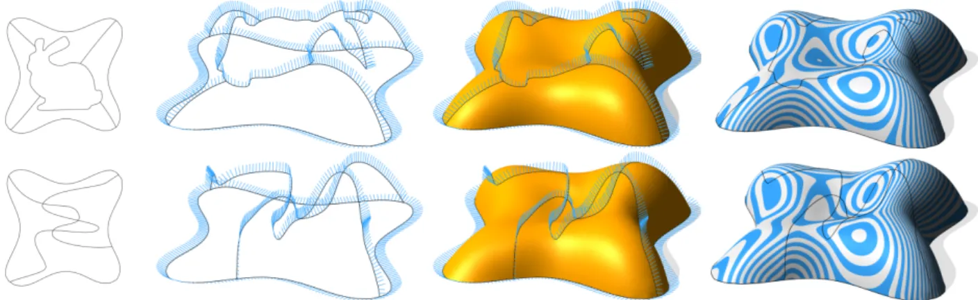
Figure 9: In terms of geometry, we place no constraints on the input. Our method can handle even these challenging networks with winding curves, all while preserving the global smoothness across patches.
San Francisco, CA, USA: Morgan Kaufmann Publishers Inc.; 2002. ISBN 1-55860-737-4.
[16] Farin G, Hansford D. Discrete Coons Patches. Computer Aided Geometric Design 1999;16(7):691 – 700.
[17] Bae SH, Balakrishnan R, Singh K. ILoveSketch: As-Natural-As-Possible Sketching System for Creating 3D Curve Models. In: UIST 08. ACM; 2008, p. 151–60.
[18] Schmidt R, Khan A, Singh K, Kurtenbach G. Analytic Draw-ing of 3D Scaffolds. ACM Trans Graph (Proc SIGGRAPH Asia) 2009;28(5):149:1–149:10.
[19] Xu B, Chang W, Sheffer A, Bousseau A, McCrae J, Singh K.
True2Form: 3D Curve Networks from 2D Sketches via
Se-lective Regularization. ACM Trans Graph (Proc SIGGRAPH) 2014;33(4):131:1–131:13.
[20] Rose K, Sheffer A, Wither J, Cani MP, Thibert B. Developable Sur-faces from Arbitrary Sketched Boundaries. In: Proc. Symp. Geom. Proc. 2007, p. 163–72.
[21] Rivers A, Durand F, Igarashi T. 3D Modeling with Silhouettes. ACM Trans Graph (Proc SIGGRAPH) 2010;29(4):1–8.
[22] Umetani N, Kaufman DM, Igarashi T, Grinspun E. Sensitive Cou-ture for Interactive Garment Modeling and Editing. ACM Trans Graph (Proc SIGGRAPH) 2011;30(4):90:1–90:12.
[23] Tasse FP, Emilien A, Cani MP, Hahmann S, Dodgson N. Feature-Based Terrain Editing from Complex Sketches. Computers & Graphics 2014;45:101 –15.
[24] Pan H, Liu Y, Sheffer A, Vining N, Li CJ, Wang W. Flow-Aligned Surfacing of Curve Networks. ACM Trans Graph (Proc SIGGRAPH) 2015;34(4):127:1–127:10.
[25] Jung A, Hahmann S, Rohmer D, Begault A, Boissieux L, Cani MP. Sketching Folds: Developable Surfaces from Non-Planar Silhou-ettes. ACM Trans Graph 2015;34(5):155:1–155:12.
[26] Nealen A, Igarashi T, Sorkine O, Alexa M. FiberMesh: Designing Freeform Surfaces with 3D Curves. ACM Trans Graph (Proc SIG-GRAPH) 2007;26(3).
[27] Stanko T, Hahmann S, Bonneau GP, Saguin-Sprynski N. Smooth interpolation of curve networks with surface normals. In: Bashford-Rogers T, Santos LP, editors. EG 2016 – Short Papers. Lisbon, Portugal: Eurographics Association; 2016, p. 21 –4. [28] Kara LB, Shimada K. Sketch-Based 3D-Shape Creation for
Indus-trial Styling Design. IEEE Computer Graphics and Applications 2007;27(1):60–71.
[29] Das K, Diaz-Gutierrez P, Gopi M. Sketching FreeForm Surfaces Us-ing Network of Curves. In: Jorge J, Igarashi T, editors. Eurograph-ics Workshop on Sketch-Based Interfaces and Modeling. 2005,. [30] Zhuang Y, Zou M, Carr N, Ju T. A General and Efficient Method
for Finding Cycles in 3D Curve Networks. ACM Trans Graph (Proc SIGGRAPH Asia) 2013;32(6):180:1–180:10.
[31] Bessmeltsev M, Wang C, Sheffer A, Singh K. Design-driven Quad-rangulation of Closed 3D Curves. ACM Trans Graph (Proc SIG-GRAPH Asia) 2012;31(6):178:1–178:11.
[32] Sadri B, Singh K. Flow-complex-based Shape Reconstruction from
3D Curves. ACM Trans Graph 2014;33(2):20:1–20:15.
[33] Schaefer S, Warren J, Zorin D. Lofting Curve Networks Using Sub-division Surfaces. In: Proc. Symp. Geom. Proc. 2004, p. 103–14. [34] Boier-Martin I, Ronfard R, Bernardini F. Detail-preserving
Varia-tional Surface Design with Multiresolution Constraints. In: Proc. Shape Modeling Applications. 2004, p. 119–28.
[35] Moreton HP, S´equin CH. Functional Optimization for Fair Surface Design. Computer Graphics (SIGGRAPH) 1992;26(2):167–76. [36] Botsch M, Sorkine O. On Linear Variational Surface Deformation
Methods. IEEE Trans Vis Comput Graphics 2008;14(1):213–30. [37] Farin G. A Construction for Visual C1 Continuity of
Polyno-mial Surface Patches. Computer Graphics and Image Processing 1982;20(7):272–82.
[38] Schneider R, Kobbelt L. Geometric Fairing of Irregular Meshes for FreeForm Surface Design. Computer Aided Geometric Design 2001;18(4):359–79.
[39] Crane K, Pinkall U, Schr¨oder P. Robust Fairing via Conformal Cur-vature Flow. ACM Trans Graph (Proc SIGGRAPH) 2013;32. [40] Shewchuk JR. Triangle: Engineering a 2D Quality Mesh Generator
and Delaunay Triangulator. In: Applied computational geometry towards geometric engineering. Springer; 1996, p. 203–22. [41] Zou M, Ju T, Carr N. An Algorithm for Triangulating Multiple 3D
Polygons. Computer Graphics Forum (SGP) 2013;32(5):157–66. [42] Meyer M, Desbrun M, Schr¨oder P, Barr AH. Discrete Differential
Geometry Operators for Triangulated 2-manifolds. In: Visualiza-tion and mathematics III. Springer; 2003, p. 35–57.
[43] Botsch M, Kobbelt L, Pauly M, Alliez P, L´evy B. Polygon Mesh Pro-cessing. CRC press; 2010.
[44] Sullivan J. Curvatures of Smooth and Discrete Surfaces. In: Bobenko A, Sullivan J, Schr¨oder P, Ziegler G, editors. Discrete Differential Geometry; Oberwolfach Seminars Vol. 38. Birkhauser Basel; 2008, p. 175–88.
[45] Grinspun E, Gingold Y, Reisman J, Zorin D. Computing Discrete Shape Operators on General Meshes. Computer Graphics Forum (Proc Eurographics) 2006;25(3):547–56.
![Figure 3: Mean curvature of the irregular horse mesh. (Left) the cotan formula [42] which is based solely on the mesh vertices, (middle & right) the 3-averaging formula (1), which additionally takes into account a normal at each vertex](https://thumb-eu.123doks.com/thumbv2/123doknet/13574482.421458/6.892.88.806.125.289/figure-curvature-irregular-formula-vertices-averaging-formula-additionally.webp)