Solutions of the Cahn–Hilliard equation with time-and space-fractional derivatives

(1)

International Journal of Nonlinear Science Vol.8(2009) No.1,pp.19-26

Solutions of the Cahn-Hilliard Equation with Time-and Space-Fractional

Derivatives

Zoubir Dahmani1 ∗_{, Maamar Benbachir}2

1_{Department of Mathematics,University of Mostaganem , Mostaganem, Algeria} 2_{Faculty of Sciences and Technology, Bechar University, Bechar, Algeria}

(Received 4 April 2009, accepted 7 July 2009)

Abstract: In this paper, by introducing the fractional derivative in the sense of Caputo, we apply the Adomian decomposition method for Cahn-Hilliard with time-and space-fractional derivative. As a result, numerical solutions are obtained in a form of rapidly convergent series with easily computable components.

Keywords: Caputo Fractional derivative; Adomian method; Cahn-Hilliard equation; Evo-lution Equations.

1 Introduction

Since the introduction by Adomian of the decomposition method [4, 5] at the begin of 1980s, the algorithm has been widely used for obtaining analytic solutions of physically significant equations [4–6, 20, 30–35]. With this method, we can easily obtain approximate solutions in the form of a rapidly convergent infinite series with each term computed conveniently[1, 2, 10, 17].

As it is known, for the nonlinear equations with derivatives of integer order, many methods are used to derive approximation solutions [3, 9, 14, 22, 27, 29]. However, for the fractional differential equations, there are only limited approaches, such as Laplace transform method [24], the Fourier transform method [21], the iteration method [25] and the operational method [23].

In recent years, considerable interest in fractional differential equations has been stimulated due to their numerous applications in the area of physics and engineering [11, 18, 36], like phenomena in electromag-netic theory, acoustics, electrochemistry and material science [12, 16, 24, 25, 36]. In [28], the Adomian decomposition method ( ADM ) is applied to the Cahn-Hilliard equation

u_t= γu_x+ 6u(u_x)2+ (3u2− 1)u_xx− u_xxxx, γ ≥ 0. (1) This equation is related with a number of interesting physical phenomena like the spinodal decomposi-tion, phase separation and phase odering dynamics. It is also very crucial in material sciences [7, 8, 15]. On the other hand this equation is very hard and difficult to solve. Many articles have investigated mathemati-cally and numerimathemati-cally this equation [13, 19].

The aim of this paper is to use the ADM method to study the Cahn-Hilliard equation with time-and space-fractional derivatives of this form

Dα_tu − γD_xβu − 6u(Dβ_xu)2− (3u2− 1)uxx+ uxxxx= 0. (2) Here α and β are the parameters standing for the order of the fractional time and space derivatives, respectively and they satisfy 0 < α ≤ 1, 0 < β ≤ 1 and x > 0. In fact, different response equations can be

∗_{Corresponding author.} _{E-mail address: zzdahmani@yahoo.fr}

Copyright c°World Academic Press, World Academic Union IJNS.2009.08.15/239

(2)

obtained when at lest one of the parameters varies. When α = β = 1, the fractional equation reduces to the Cahn-Hilliard equation (1).

We introduce Caputo fractional derivative and apply the ADM to derive numerical solutions of the equation (2).

The paper is organized as follows. In SecII, some necessary details on the fractional calculus are pro-vided. In SecIII, the Cahn-Hilliard equation with time and space-fractional derivative is studied with the ADM. Finally, conclusions follow.

2 Description of Fractional Calculus

There are several mathematical definitions about fractional derivative [24, 25]. Here, we adopt the two usually used definitions: the Caputo and its reverse operator Riemann-Liouville. That is because Caputo fractional derivative allows traditional initial condition assumption and boundary conditions. More details one can consult [24]. In the following, we will give the necessary notation and basic definitions.

Definition 1 A real valued function f (x), x > 0 is said to be in the space Cµ, µ ∈ IR if there exists a real

number p > µ such that f (x) = xp_f

1(x) where f1(x) ∈ C([0, ∞)).

Definition 2 A function f (x), x > 0 is said to be in the space Cn

µ, n ∈ IR, if f(n)∈ Cµ.

Definition 3 The Riemann-Liouville fractional integral operator of order α ≥ 0, for a function f ∈ C_µ, (µ ≥ −1) is defined as Jα_{f (x) =} 1 Γ(α) R_x 0(x − t)α−1f (t)dt; α > 0, x > 0 J0_{f (x) = f (x).} (3)

For the convenience of establishing the results for the Cahn-Hilliard equation, we give one basic prop-erty:

JαJβf (x) = Jα+βf (x). (4) For the expression (3), when f (x) = xβ_{we get another expression that will be used later:}

Jαxβ = Γ(β + 1) Γ(α + β + 1)x

α+β_. ₍₅₎

Definition 4 The fractional derivative of f ∈ Cn

−1in the Caputo’s sense is defined as

Dαf (t) = ( 1 Γ(n−α) R_t 0(t − τ )n−α−1f(n)(τ )dτ, n − 1 < α < n, n ∈ IN∗, dn dtnf (t), α = n. (6)

According to the Caputo’s derivative, we can easily obtain the following expressions:

Dα_{K = 0; K is a constant.} Dαtβ = ( Γ(β+1) Γ(β+1−α)tβ−α, β > α − 1, 0, β ≤ α − 1. (7)

Details on Caputo’s derivative can be found in [24].

Remark 1 In this paper, we consider equation (2) ( with time-and space fractional derivatives). When α ∈ IR+_{, we have:} D_tαu(x, t) = ∂ α_{u(x, t)} ∂tα = ( 1 Γ(n−α) R_t 0(t − τ )n−α−1 ∂ n_{u(x,τ )} ∂τn dτ, n − 1 < α < n ∂n_u(x,t) ∂tn , α = n. (8)

(3)

3 Applications of the ADM Method

Consider the Cahn-Hilliard equation with time and space-fractional derivatives Eq.(2). In order to solve numerical solutions for this equation by using ADM method, we rewrite it in the operator form:

Dα_tu = γD_xβu + 6u(Dβ_xu)2+ (3u2− 1)u_xx− u_xxxx, β > 0, α > 0, γ > 0, (9) where the operators Dα

t and Dxβstand for the fractional derivative and are defined as in (6). Take the initial condition as

u(x, 0) = f (x). (10)

Applying the operator Jα_{, the inverse of D}α _{on corresponding sub-equation of Eq.(9), using the initial} condition ( 10), yields:

u(x, t) = f (x) + γJαΦ1(u(x, t)) + 6JαΦ2(u(x, t)) + JαΦ3(u(x, t)) − JαL(u(x, t), (11)

where Φ1(u) = Dxβu, Φ2(u) = u(Dxβu)2, Φ3(u) = (3u2− 1)uxx, L(u(x, t)) = uxxxx.

Following Adomian decomposition method [4, 5], the solution is represented as infinite series like

u(x, t) =

∞ X n=0

un(x, t). (12)

The nonlinear operators Φ1(u), Φ2(u) and Φ3(u) are decomposed in these forms

Φ1(u) = ∞ X n=0 An, Φ2(u) = ∞ X n=0 Bn, Φ3(u) = ∞ X n=0 Cn, (13)

where An, Bn, Cnare the so-called Adomian polynomials and have the form

An= _n!1 d n dλn " Φ1 Ã _∞ X k=0 λkuk !# λ=0 = 1 n! dn dλn " Dβ_x Ã _∞ X k=0 λkuk !# λ=0 , (14) Bn= _n!1 d n dλn " Φ2 Ã_∞ X k=0 λkuk !# λ=0 = 1 n! dn dλn   Ã_∞ X k=0 λkuk ! Ã Dβ_x ∞ X k=0 λkuk !₂  λ=0 , (15) Cn= _n!1 d n dλn    3 Ã _∞ X k=0 λkuk !₂ − 1   Ã _∞ X k=0 λkukxx !  λ=0 .

In fact, these Adomian polynomials can be easily calculated. Here we give the first three components of these polynomials:

A0 = Dβxu0, A1= Dxβu1,

A2 = Dβxu2, A3= Dxβu3.

(16) The first three components of Bnare

B₀= u₀(Dβxu0)2, B1 = 2u0Dxβu0Dβxu1+ (Dβxu0)2u1,

B2= 4u0Dβxu0Dxβu2+ 2u0(Dβxu1)2+ 3u1Dβxu0Dβxu1+ u2(Dxβu0)2,

B3= 1₃(12u0Dxβu1Dxβu2+ 5u1(Dxβu1)2+ 10u1Dβxu0Dβxu2+

+12u₀Dβxu0Dβxu3+ 6u2Dxβu0Dxβu1+ 2u1u2Dxβu0+ 3u3(Dxβu0)2).

(17)

and those of Cnare given by:

C0= 3u20u0xx− u0xx, C1= 3(2u0u1u0xx+ u20u1xx) − u1xx,

C2 = 3(u21u0xx+ 2u0u2u0xx+ 2u0u1u1xx+ u20u2xx) − u2xx,

C3 = 3((2u1u2+ 2u0u3)u0xx+ (u21+ 2u0u2)u1xx+ 2u0u1u2xx+ u20u3xx) − u3xx.

(4)

Other polynomials can be generated in a like manner. Substituting the decomposition series (12) and (13) into Eq.(11), yields the following recursive formula:

u₀(x, t) = f (x), u_n+1(x, t) = γJα(A_n) + 6Jα(B_n) + Jα(C_n) − Jα(L_x(u_n)); n ≥ 0. (19) The Adomian decomposition method converges generally very quickly. Details about its convergence and convergence speed can be found in [1, 2, 10, 17]. Here, according to the above steps, we will derive the numerical solution for the Eq.(9) in details.

3.1 Numerical Solutions of Time-Fractional Cahn-Hilliard Equation Consider the following form of the time-fractional equation (for γ = 1)

Dα_tu = u_x+ 6u(u_x)2+ (3u2− 1)u_xx− u_xxxx, (20) with the initial condition [28]

u(x, 0) = f (x) = tanh( √

2

2 x), (21)

The exact solution of (20) for the special case α = β = 1 is :

u(x, t) = tanh( √

2

2 (x + t)). (22)

In order to obtain numerical solution of equation (20), substituting the initial condition (21) and using the Adomian polynomials (15-18) into the expression (19), we can compute the results. For simplicity, we only give the first few terms of series:

u0 = tanh( √ 2 2 x), u1 = Jα(A0) + 6Jα(B0) + Jα(C0) − Jα(u0xxxx) = Jα(u0x) + 6Jα(u0u20x) + Jα(3u20u0xx− u0xx) − Jα(u0xxxx) = f1 t α Γ(α + 1), u2 = Jα(A1) + 6Jα(B1) + Jα(C1) − Jα(u1xxxx) = Jα(u1x) + 6Jα(2u0u0xu1x+ (u0x)2u1) + Jα(3(2u0u1u0xx+ u20u1xx) − u1xx) − Jα(u1xxxx) = f2 t 2α Γ(2α + 1), u3 = Jα(A2) + 6Jα(B2) + Jα(C2) − Jα(u2xxxx) = Jα(u2x) + 6Jα(4u0u0xu2x+ 2u0(u1x)2+ 3u1u0xu1x+ u2(u0x)2) + Jα(3(u2₁u0xx+ 2u0u2u0xx+ 2u0u1u1xx+ u20u2xx) − u2xx) − Jα(u1xxxx) = f₃ t3α Γ(3α + 1), (23) where f (x) = u₀= tanh( √ 2 2 x), (24) f1(x) = fx+ 6f fx2+ (3f2fxx− fxx) − fxxxx, (25) f2(x) = f1x+ 6(2f fxf1x+ f2f1) + 3(2f f1fxx+ f2f1xx) − f1xx− f1xxxx, (26) f3(x) = f2x+ 6(4f fxf2x+ 2f (f1x)2 Γ(2α+1)_Γ2_(α+1) + 3f1fxf1xΓ(2α+1)_Γ2_(α+1) + f2(fx)2)+ +(3(f₁2fxxΓ(2α+1)_Γ2_(α+1) + 2f f2fxx+ 2f f1f1xx Γ(2α+1) Γ2_(α+1) + f2f2xx) − f2xx) − f1xxxx. (27)

(5)

Then we have the numerical solution of time-fractional equation (20) under the series form u(x, t) = f (x) + f₁(x) tα Γ(α + 1) + f2(x) t2α Γ(2α + 1)+ f3(x) t3α Γ(3α + 1)+ ... (28) In order to check the efficiency of the proposed ADM for the equation (20), we draw figures for the numerical solutions with α = 1₂ as well as the exact solution (22) when α = β = 1. Figure(a) shows the exact solution. Figure(b) stands for the numerical solution (28). From these figures, we can appreciate how closely are the two solutions. This is to say that good approximations are achieved using the ADM method.

Figure 1: Exact solution of Eq.(20)

Figure 2: Solution of Eq.(20)obtained by ADM method for α = 1₂

3.2 Numerical Solutions of Space-Fractional Cahn-Hilliard Equation

In this section, we will take the space-fractional equation as another example to illustrate the efficiency of the method. As the main computation method is the same as the above, we will omit the heavy calculation and only give some necessary expressions.

Considering the operator form of the space-fractional equation (for γ = 1)

ut= Dβxu + (3u2− 1)uxx+ 6u(Dxβu)2− uxxxx, 0 < β < 1. (29) Assuming the initial condition as

u(x, 0) = f (x) = x2. (30) Initial condition has been taken as the above polynomial to avoid heavy calculation of fractional differ-entiation.

In order to estimate the numerical solution of equation (29), substituting (15-17) and the initial condition (30) into (19), we get the Adomian solution. Here, we give the first few terms of the series solution:

u0 = f (x) = x2,

u₁ = J(A₀) + 6J(B₀) + J(C₀) − J(D₀)

= J(Dβ_xu₀) + 6J(u₀(D_xβu₀)2) + J(3u2₀u_0xx− u_0xx) − J(u_0xxxx) = (f1x2−β+ f2x6−2β+ 6x4− 2)t, u₂ = J(A₁) + 6J(B₁) + J(C₁) − J(L_x(u₁)) = J(Dβ_xu1) + 6J ³ 2u0Dxβu0Dxβu1+ (Dxβu0)2u1 ´ + J¡3(2u0u1u0xx+ u20u1xx) − u1xx ¢ − J (u1xxxx) = t 2 2 (f3(x) + 6f4(x) + f5(x) − f6(x)) (31)

(6)

where f (x) = x2, f1 = Γ(3) Γ(3 − β), f2= 6Γ2₍₃₎ Γ2_{(3 − β)}, f3(x) = f1_{Γ(3 − 2β)}Γ(3 − β) x2−2β+ f2Γ(7 − 2β)_{Γ(7 − 3β)}x6−3β+ 6_{Γ(5 − β)}Γ(5) x4−β (32) f4(x) = 2f1_Γ(3−2β)Γ(3) x6−3β+ 2f2_{Γ(3−β)Γ(7−3β)}Γ(3)Γ(7−2β) x8−3β +12_{Γ(5−β)Γ(3−β)}Γ(3)Γ(5) x6−β₊ Γ2(3) Γ2_(3−β)(f1x6−3β+ f2x10−4β + x8−2β− 2x4−2β), (33) f5(x) = 12f1x4−β + 12f2x8−2β+ 72x6− 24x2+ 3(2 − β)(1 − β)f1x4−β +3(6 − 2β)(5 − 2β)f2x8−2β+ 3.72x6+ −(2 − β)(1 − β)f1x−β− (6 − 2β)(5 − 2β)f2x4−2β− 72x2, f6(x) = (2 − β)(1 − β)(−β)(1 − β − 1)f1x−2−β+ (6 − 2β)(5 − 2β)(4 − 2β)(3 − 2β)f2x2−2β. (34)

Then we obtain a numerical solution of space-fractional equation (29) in series form

u(x, t) = x2_{+ t}¡_f

1x2−β+ f2x6−2β+ 6x4− 2

¢ +t2

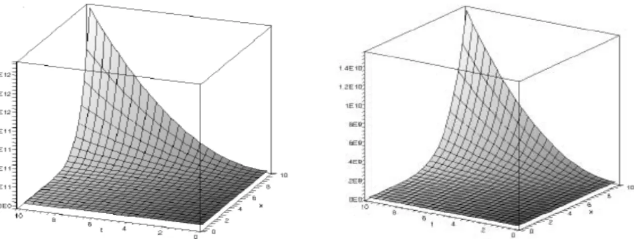
2 (f3(x) + 6f4(x) + f5(x) − f6(x)) + ... (35) Figures(c,d) show, respectively, the numerical solutions given by expression (35) for the equation (29) with β = 1

2 and β = 1. From these figures, we can appreciate the convergence rapidity of Adomian

solutions.

Figure 3: Solution of Eq.(29) obtained by ADM method for β = 1

2.

Figure 4: Solution of Eq.(29)obtained by ADM method for β = 1.

4 Conclusion

In this paper, the ADM has been successfully applied to derive explicit numerical solutions for the time-and space-fractional Cahn-Hilliard equation. The above procedure shows that the ADM method is efficient and powerful in solving wide classes of equations in particular evolution fractional order equations.

References

[1] K. Abbaoui, Y. Cherruault: Convergence of Adomian’s method applied to differnetial equations.

Com-put. Math. Appl. 28(5):103-109 (1994)

[2] K. Abbaoui, Y. Cherruault: New ideas for proving convergence of decomposition method. Comput.

(7)

[3] M.J. Ablowitz, P.A. Clarkson: Solitons, nonlinear evolution equations and inverse scatting. Cambridge

University Press, New York. (1991)

[4] G. Adomian: Nonlinear stochastic Systems theory and applications to Physics. Kluwer Academic

Pub-lishers, Dordrecht. (1989)

[5] G. Adomian: Solving frontier problems of Physics: The decomposition method. Kluwer Academic

Publishers, Boston. (1994)

[6] E. Baboblian, A. Davari: Numerical implementation of A domian decomposition method for linear Volterra integral equation of the second kind. Appl. Math. Comput. 165: 223-227 (2005)

[7] J.W. Chan: On spinodal decomposition. Acta Metall. 9: 795-803 (1961)

[8] S.M. Choo, S. K. Chung, Y.J. Lee: A conservative difference scheme for the viscous Cahn-Hilliard with a nonconstant gradient energy coefficient.Appl. Numb. Math. 51: 207-219 (2004)

[9] Y. Chen, Y.Z. Yan: Weierstrass semi rational expansion method and new doubly periodic solutions of the generalized Hirota-Satsuma coupled KdV system. Appl. Math. Comput. 177:85-91 (2006)

[10] Y. Cherruault: Convergence of Adomian’s method .Kybernetes. 18:31-38 (1989)

[11] V. Daftardar-Gejji, H. Jafari. Adomian decomposition: A tool for solving a system of fractional differ-ential equations. J. Math. Anal. Appl. 301:508-518 (2005)

[12] Z. Dahmani, M. M. Mesmoudi, R. Bebbouchi: The foam-drainage equation with time and space frac-tional derivative solved by the ADM method. E. J. Qualitative Theory of Diff. Equ.30:1-10 (2008) [13] E.V.L. De Mello, T. Otto, F. Da Silveira: Numerical study of the Cahn-Hilliard equation in one, two

and three dimensions. Physica A.347, 429-443 (2005)

[14] E. Fan: Extended tanh function method and its applications to nonlinear equations. Phys. Lett.

A.277:212-218 (2000)

[15] M. Gurtin: Generalised Ginzburg-Landau and Cahn-Hilliard equations based on a microforce balance.

Physica D.92: 178-192 (1996)

[16] J.H. He: Some applications of nonlinear fractional differential equations and their approximations.

Bull. Sci. Techno. 15(2): 86-90 (1999)

[17] N. Himoun, K. Abbaoui, Y. Cherruault: New results of convergence of Adomian’s method. Kybernetes. 28(4-5): 423-429(1999)

[18] H. Jafari, V. Daftardar-Gejji: Solving a system of nonlinear fractional differential equations using Adomian decomposition. J. Comput. Appl. Math. 196: 644-651 (2006)

[19] K. Junseok: A numerical method for the Cahn-Hilliard equation with a variable mobility.Commun.

Nonlinear Sci. Numer. Simul. 12: 1560-1572 (2007)

[20] D. Kaya, S.M. El Sayad: A numerical implementation of the decomplosition method for the Lienard equation. Appl. Math. Comput. 171:1095-1103(2005)

[21] S. Kemple, H. Beyer: Global and causal solutions of fractional differential equations in : Transform Method and Special Functions . Varna96, Proceding of the 2nd International Workshop (SCTP),

Sin-gapore. (1997)

[22] Y. Luchko, R. Gorenflo: The initial value problem for some fractional differential equations with the Caputo derivaitve. Preprint Series A 08-98, Fachbereich Mathematik und Informatik, Freie Universitat

(8)

[23] Y. Luchko, H.M. Srivastava: The exact solutions of certain differential equations of fractional order by using operational calculus. Comput. Math. Appl. 29:73-85 (1995)

[24] I. Podlubny: Fractional Differential Equations. Academic Press, San Diego.(1999)

[25] G. Samko, A.A. Kilbas, O.I. Marichev: Fractional integral and derivative: Theory and Applications .

Gordon and Breach, Yverdon. (1993)

[26] S M. El- Sayed, D. Kaya: An application of ADM to seven-order Sawada-Kotara equations. Appl.

Math. Comput. 157:93-101 (2004)

[27] S. Momani, Z. Odibat: Numerical approach to differential equations of fractional order. J. Comput.

Appl. Math. 207:96-110 (2007)

[28] Y. Ugurlu, D. Kaya: Solutions of the Cahn-Hilliard equation. Comput. Math. Appl. 56 :3038-3045(2008)

[29] Q. Wang: Numerical solutions for fractional KdV-Burgers equation by Adomian decomposition method. Appl. Math. Comput. 182: 1049-1055 (2006)

[30] A.M. Wazwaz: A new approch to the nonlinear advection problem. Appl. Math. Comput. 72: 175-181(1995)

[31] A.M. Wazwaz: A reliable modification of Adomian decomposition method. Appl. Math. Comput. 102:77-86 (1999)

[32] A.M. Wazwaz: A new algorithm for calculating Adomian polynomials for nonlinear operators. Appl.

Math. Comput. 111:53-69 (2000)

[33] A.M. Wazwaz: A computational approach to solitons of the Kadomtsev-Petviashvili equation. Appl.

Math. Comput. 123: 205-217 (2001)

[34] A.M. Wazwaz: Partial differential equations: Methods and Applications.Balkema Publishers. The

Netherlands. (2002)

[35] A.M. Wazwaz, A. Georguis: An analytic study of Fisher’s equations by using Adomian decomposition method. Appl. Math. Comput. 154:609-620 (2004)