A new parameter to empirically describe and predict the non-linear seismic response of sites derived from the analysis of Kik-Net database

HAL Id: hal-02418730

https://hal.archives-ouvertes.fr/hal-02418730

Submitted on 26 Nov 2020

HAL is a multi-disciplinary open access

archive for the deposit and dissemination of

sci-entific research documents, whether they are

pub-lished or not. The documents may come from

teaching and research institutions in France or

abroad, or from public or private research centers.

L’archive ouverte pluridisciplinaire HAL, est

destinée au dépôt et à la diffusion de documents

scientifiques de niveau recherche, publiés ou non,

émanant des établissements d’enseignement et de

recherche français ou étrangers, des laboratoires

publics ou privés.

A new parameter to empirically describe and predict the

non-linear seismic response of sites derived from the

analysis of Kik-Net database

David Castro-Cruz, Julie Regnier, Etienne Bertrand, Françoise Courboulex

To cite this version:

David Castro-Cruz, Julie Regnier, Etienne Bertrand, Françoise Courboulex. A new parameter to

empirically describe and predict the non-linear seismic response of sites derived from the analysis

of Kik-Net database. Soil Dynamics and Earthquake Engineering, Elsevier, 2020, 128, pp.105833.

�10.1016/j.soildyn.2019.105833�. �hal-02418730�

A new parameter to empirically describe

1

and predict the non-linear seismic

2

response of sites derived from the

3

analysis of Kik-Net database

4 5 6

Authors 7

David Castro-Cruza,b,*_{, Julie Régnier}a_{, Etienne Bertrand}a_{, Françoise Courboulex}b

8

a _{CEREMA, Agence de Sophia Antipolis, 06903 Valbonne, France}

9

b _{Université Côte d'Azur, CNRS, Observatoire de la Côte d'Azur, IRD, Géoazur, 06560 Valbonne, France}

10

Email addresses: 11

david.castro@cerema.fr (D. Castro-Cruz) , julie.regnier@cerema.fr (J. Régnier), etienne.bertrand@cerema.fr 12

(E. Bertrand), courboulex@geoazur.unice.fr ( F. Courboulex) 13

Corresponding author: David Castro-Cruz 14

Abstract

15

We evaluate the non-linear site response at the stations of the Japanese Kik-Net network by computing the ratio 16

between the Fourier spectra of the recordings at the surface and at the downhole station. When the amplitude 17

of the input signal increases, we observe a shift of the resonance peaks towards lower frequencies, characteristic 18

of non-linear soil behavior. We propose a new parameter called fsp to characterize this shift. We observe that 19

fsp is a good proxy for the shear modulus reduction by comparing fsp and the modulus reduction curve obtain 20

by both laboratory test measurements and numerical approaches. The fsp is used to correct the linear site 21

response and surface ground motion in frequency domain in order to take into account the non-linear soil 22

behavior. We show that the procedure we established reduces the error in predicting the main frequency peak 23

by 50% compared to an elastic evaluation of the site response during the 2016 Kumamoto earthquake 24

(Mw=7.1). 25

26

Keywords: Non-linear site behavior; site effect; Kik-net; Ground motion prediction; Kumamoto Earthquake

27 28

Highlights:

29

• Quantification of non-linear site effects during a ground motion. 30

• Quantification of the propensity of a site to develop non-linear site effects. 31

• Prediction of strong motion during the Kumamoto 2016 (Mw 7.1) earthquake. 32

• A parameter based on borehole recordings to quantify non-linear site behavior. 33

Funding: This research has been funded by a PhD Grant and work environment from CEREMA.

34

© 2019. This manuscript version is made available under the Elsevier user license https://www.elsevier.com/open-access/userlicense/1.0/

Version of Record: https://www.sciencedirect.com/science/article/pii/S0267726118304159

1

Introduction

35

It is widely recognized that soft soils can amplify dramatically the seismic motion compared to rock reference 36

site because of seismic waves being trapped in sub-surface sedimentary layers [1–3]. The seismic site response 37

depends on the site geometric configuration, the nature of the soil and the incoming ground motion [4]. For 38

weak ground motion, the combination of a complex site configuration and various incident wave field induces 39

a variability on the site response [5]. For strongest ground motions, the soil non-linear behavior can, in 40

addition, have a strong influence on the site response [6,7]. An accurate prediction of strong ground motion 41

on sedimentary site will, therefore, require the consideration of non-linear soil behavior. 42

In laboratories, under cyclic and seismic loading, the soil non-linear behavior is illustrated in terms of 43

hysteretic loops in the stress-strain plan [8,9]. The effects of non-linearity in the soil mechanical behavior are 44

generally a reduction of the shear modulus with increasing strain and an increase of the dissipation of energy 45

within the material. Consequently, the hysteretic behavior of the soil can be recovered knowing the shear 46

modulus reduction curve (G/Gmax) and the damping (ξ) curves .

47

For the transfer function, that quantify the site response, the effects of the non-linear soil behavior leads in a 48

shift of the resonance frequencies of the site towards lower frequency, induced by a decrease of the apparent 49

shear wave velocity, associated in most of the cases to an attenuation of the high frequency amplifications 50

[10]. Nevertheless, an increase of the amplification at high frequency has been also sometimes reported, 51

which was associated with a decrease of the pore water pressure when cyclic mobility occurs [11] or soil 52

hardening [12]. Many studies show that these differences are larger when the intensity of the incident motion 53

increases (e.g. [13–15]). 54

The non-linear soil parameters can be characterized by various methods from laboratory testing on soil 55

samples to lower cost method based on correlations between non-linear parameters and other soil 56

parameters (e.g. [16,17]). In-situ measurements can also be used in addition to laboratory tests to infer these 57

non-linear parameters. Some authors use accelerometric data to determine the shear modulus reduction and 58

damping curves. These parameters are often estimated by finding the best numerical model that reproduces 59

the accelerometric time histories. It has been applied mainly in Taiwan and in Japan (e.g. [18–20]). Other 60

authors use interferometry between recordings at different depth to derive the instantaneous wave 61

propagation velocity in the media depending on the input motion intensity [21,22]. 62

Another way to study soil non-linear behavior is to compare site-response curves computed from weak motion 63

and strong motion. In Noguchi and Sasatani [23] the ratio between the Fourier spectrum of records at the 64

surface and at downhole (BSR) are computed. They compared BSR from weak and strong ground motion by 65

the summation of the differences at each frequency between each BSR, parameter that was called DNL 66

(Degree of Non-linearity). They showed a link between the nonlinear effects (defined as DNL), and an intensity 67

parameter of the shaking (PGA). In Lussou et al. [24] and Régnier et al. [7], several parameters are proposed 68

to quantify those differences, such as an estimation of the modification of the BSR curves and a measurement 69

of the frequency shift. In Field et al. [25] ratios between spectral ratios were computed using synthetic rock 70

reference seismograms. Similarly, in Régnier et al. [10] the ratio of the non-linear to linear spectral ratios are 71

analyzed, but using vertical arrays. In all cases, the authors found that the non-linear to linear site response 72

discrepancy is related to the frequency range and increase with increasing PGA of the incident ground motion. 73

Following a similar approach, we compare weak motion and strong motion site responses in order to propose 74

a methodology for correcting the linear site response in order to reproduce the effects of non-linear soil 75

behavior based on the analysis of recordings from vertical arrays of the Japanese Kiban Kyoshin network (KiK-76

Net). After a description of our approach, an application will be detailed on the recordings of the 2016 77

Kumamoto Japanese earthquake. 78

2

Data

79

To study the influence of the non-linearity of the soil behavior on the empirical BSR, we use the KiK-net dataset 80

in Japan. These data are available on the web page of the National Research Institute for Earth Science and 81

Disaster Prevention (http://www.kyoshin.bosai.go.jp). The network is composed of 688 stations, among them, 82

650 sites are characterized with Vs and Vp profiles, soil description, and information on the stations (location 83

and information of recording devices). For each recorded earthquake, the acceleration time histories are 84

provided, with the event origin time, the epicenter location, the depth of the hypocenter, and the magnitude 85

of the earthquake determined by the Japanese Meteorological Agency. 86

We selected recordings according to two criteria: signals from earthquakes with a magnitude higher than 3 87

and with an epicentral distance lower than 500 km. Under those two criteria, we use 75 232 signals (each one 88

recorded in the three directions at the surface and at downhole) from 5 535 earthquakes with magnitudes 89

between 3 and 9, recorded between November 1997 to December 2017. Figure 1 presents the whole selected 90

records used in our analysis. 91

92

Figure 1. Magnitude/distance distribution of earthquakes recordings used in this study.

93

Subsequently, for all of the selected seismograms a signal processing based on Boore [26] recommendations 94

was applied. It consists in: (1) removing the mean, (2) removing the data before the first zero-crossing point, 95

(3) Applying an Hanning’s window to improve the trimming process of the signal [27], and finally (4) Applying 96

two times a high pass filter of 2nd order with fc=0.1 Hz. This processing allows to remove the low-frequency 97

noise and to ensure compatibility between acceleration, velocity and displacement time series and Fourier 98

and response spectra. In particular, effects of spurious low frequency can be removed from the data through 99

this procedure. 100

The empirical site response is assessed on the horizontal components by computing the Borehole Spectral 101

Ratios (BSR), defined as the ratio between the geometric average of the Fourier amplitude spectra of the 102

horizontal components at the surface and at downhole (Equation (1)). 103 ( ) = 2

₊

₊

Where EW and NS are the amplitude of the Fourier transform of the accelerograms for East-West, and North-104

south horizontal components respectively. In this study, we applied a Konno-Ohmachi smoothing [28] to each 105

spectrum, improving the comparison between spectra and avoiding zero values at the denominator of 106

(Equation (1)). BSR shows, in the frequency domain, how the seismic signal varies between the downhole 107

sensor and the one at the surface. BSR curves indicate the site resonance frequencies f(n) _{if the downhole}

108

sensor is located at the main sediment to substratum interface. Otherwise, the curve includes pseudo-109

resonances that are induced by the destructive interferences of the down-going waves with the incident ones 110

at the downhole sensor [29]. However, the comparison of weak and strong site response remains relevant to 111

characterize non-linear site behavior. 112

3

Method

113

Our method defines a parameter called fsp that characterize the non-linear site behavior. To illustrate our 114

methodology, we detail the whole procedure on one site of the KiK-net database (IBRH11) that has recorded 115

both weak and strong ground motions. Then, we compare the parameter fsp to laboratory data (shear 116

modulus reduction curves) obtained from cyclic tri-axial test at one Kik-net site (KSRH10), that was 117

characterized during a previous PRENOLIN project [30]. Finally, the parameter is tested analytically by using 118

non-linear site response calculations on simple site configuration (1-D, non-linear, mono-layer cases). 119

120

3.1

fsp: a new parameter to characterize non-linear site behavior

121

In order to explain our methodology, we detail the whole method on one site of the KiK-net database that has 122

recorded a large panel of earthquakes from weak to strong motions. Then, we will generalize the procedure 123

to all of the stations. Station IBRH11 has recorded 515 earthquakes and it is located in the prefecture of Ibaraki 124

(Figure 2) on a D-site according to the Eurocode 8 (EC8) with a Vs30 of 242 m/s ( = 30 ∑ℎ / ) and a

125

depth of 103 meters. The bedrock is reached at 30m depth and is characterized with a Vs of 2100 m/s. The 126

downhole station is situated at 100m depth. 127

128

Figure 2. Location and Vs profiles of stations IBRH11 and KSRH10 and the other stations (Japanese

129

Kik-net network).

130

Figure 3 illustrates four BSR computed at IBRH11 from ground motions with different levels (PGAdownhole). We

131

observe that weak ground motions share a similar BSR. This is because for weak ground motion the site 132

response is linear [13]. The variability that can still be observed in the site response for these small seismic 133

solicitations is mainly due to complex site geometry associated to the distribution of earthquake sources 134

around the site [5]. For stronger ground motions, the peak frequencies occur at a lower frequency bandwidth. 135

We interpret this shift as a direct effect of the shear modulus reduction of the soil when the seismic solicitation 136

increases. Furthermore, the decrease in the amplitude of BSR is another effect of non-linear soil behavior 137

linked to the increase of damping with shear strain, but in the following we will only discuss about the 138

frequency shift impact. 139

140

Figure 3. BSR at IBRH11 station (KiK-net) for four earthquakes with different PGA at the downhole

141

station.

142

The weak ground motions for which the site behaves linearly are selected based on their maximal peak 143

accelerations. Indeed, the ground motions with a PGAdownhole from 10-4 m/s2 to 6. 10-3 m/s2 are considered.

144

Figure 4 presents the BSRlinear with a dotted line. It is the arithmetic average of all of the weak ground motions

145

BSR (grey curves). The black line represents the BSR computed from a strong ground motion with PGAdownhole

146

of 2.6 m/s2_{. It is easy to appreciate that the resonance peaks of the BSR from this strong ground motion are}

147

shifted to lower frequencies and that their amplitude are the smallest. 148

149

Figure 4. Definition of BSRlinear as the average of all of the weak ground motions (142 events) and

150

comparison between BSRlinear with the BSR computed from one strong ground motion.

151

BSRlinear is compared to each BSR from all of the recorded ground motions, allowing us to define a parameter

152

that characterizes the observed frequency shift. The logarithmic frequency shift is the gap in logarithmic scale 153

between BSRlinear and BSR. In linear scale, it is a coefficient that changes the frequency scale. The algorithm to

154

find this logarithmic shift minimizes the misfit between BSRlinear and BSR as defined in the Equation (2). Note

155

that the misfit is weighted by the logarithmic sampling. 156

= ! " # $%&'( ̅ _{* , −} . ̅/" ∆1

∆1 = 2345 ( 65/ ) 78 ̅ = 0.5 ∙ ( 65+ )

(2)

In the Equation (2) Ls is the logarithmic shift applied to BSRlinear. The misfit is defined as a discrete

157

approximation of the area between the shifted BSRlinear and BSR, considering a logarithmic scale as the length

158

of the base (∆x). The computation is done over a frequency window going from 0.3 Hz to 30 Hz. 159

Finally, we define a frequency shift parameter, so called fsp, as the square of the Ls, which produces the 160

minimum value of misfit (fsp=Ls2 _{when misfit is minimized). The fsp is a coefficient that is applied to the linear}

161

resonance frequency to obtain the non-linear ones for a specific ground motion. It means that if no shift is 162

needed to fit both curves, both Ls and fsp are equal to one. If BSRlinear needs to be logarithmically shifted to

163

higher frequencies to fit BSR, fsp will be higher than one. In the opposite case, fsp will be lower than one. Non-164

linear soil behavior is expected to shift the BSR to lower frequency range and therefore linked to an fsp below 165

one. 166

fsp is computed for every recording collected at station IBRH11. The results (Figure 5) shows the evolution of

167

fsp in function of the ground motion intensity, expressed in terms of the PGA recorded at the downhole

168

station. For small PGA, fsp is close to 1, but as the solicitation level increases, the value starts to decrease. The 169

decrease is gentle for PGA smaller than 0.1 m/s2 _{but is growing rapidly for larger seismic solicitations. A}

170

hyperbolic curve is used to fit the fsp values (Equation (3)), with a formulation equivalent to the one used to 171

describe the modulus reduction curves [31,32]. 172

= 5

56_{<=>FEG?@ABC@DE}<=>?@ABC@DE (3)

Where HIJ_K%LMNO$PN#% is a parameter that describes the hyperbolic function for each site. It is equal to the 173

PGAdownhole corresponding to fsp=0.5, this parameter being the counterpart of γref in the hyperbolic models

174

and the only parameter that is needed to fully describe the hyperbolic function. In order to quantify the 175

variability of fsp, a single standard deviation is computed for each station considering the whole number of 176

data. The dashed lines on Figure 5 represents the mean plus or minus one standard deviation. 177

Here, PGAdownhole can be considered as an estimator of the strain level that the site can experience during each

178

earthquake. Others proxy of strains have already been proposed in the literature. For example, Chandra [33] 179

proposed PGV/VS30 as a strain proxy. We decided to use first the PGA recorded at the downhole station

180

instead because the integration from acceleration to velocity may add some uncertainties in the PGV 181

calculation. Also PGA is a relevant parameter for describing the amount of non-linearity a soil may produce 182

[7]. 183

Figure 5. fsp value against PGA at downhole (fsp curves). Black line best hyperbolic function that fits

185

the data. Station IBRH11 - VS30: 242 m/s.

186 187

3.2

fsp parameter compared to the shear modulus reduction curves

188

We compute the fsp parameter for the earthquakes recorded at station KSRH10. This site is situated in the 189

Hokkaido prefecture, has recorded 283 events, and is located on a D-site according to EC8 (Vs30 of 212 m/s).

190

This station is particularly interesting because it has been well characterized by in-situ and laboratory data 191

measurements performed during the PRENOLIN project [30]. We plot the fsp values computed for this site 192

against the PGV at the surface divided by Vs30, as a proxy for strain, to compare with the shear modulus

193

reduction curves obtain from cyclic tri-axial tests performed at this station (Figure 5). We observe that the fsp 194

values are in the range of the shear modulus reduction curves. From this comparison we are convinced that 195

fsp is a good proxy for the shear modulus reduction with shear strain.

196

197

Figure 6: Shear modulus reduction curves defined in the PRENOLIN project at station KSRH10 (green

198

lines) at different depths from cyclic triaxial tests and fsp against PGV/ Vs30 calculated at the site.

199

The color version of this figure is available only in the electronic edition.

200 201

3.3

Comparison with analytical and numerical modeling

202

We also test fsp analytically and with numerical modeling. First, we analyze the fsp analytically in a very simple 203

case and then we apply our calculations to a more complex wave propagation in truly non-linear soil model. 204

In linear domain with 1-D configuration of a mono-layer soil and considering vertical incidence of the shear 205

waves, the resonance frequencies (f{n}_{) depend on the shear velocity (Vs) and the layer thickness (H) through}

206

f{n}_{=Vs(1+2n)/(4H). The shear velocity (V}

s) can be expressed as a function of the shear modulus as Q_R= SI T⁄

207

where G and ρ are the shear modulus and the density respectively. The shear modulus of the layer can thus 208

be derived knowing the associated resonance frequencies using the Equation (4). 209

I = (2 ∙ V ∙ {$}Y_{(0.5 + 8)},ZT (4)

210

In the equivalent linear approximation (EQL), the nonlinearity of the soil behavior is taken into account in an 211

iterative process that adjusts the elastic properties to the level of strain induced in the layer, knowing both 212

the modulus reduction and the attenuation curves. In this frame, the shear modulus at a linear strain rate 213

(Gmax) can be compared to the shear modulus at larger strain (G), by the ratio between both. Using the

214

Equation (4) for both modulus, the ratio will be expressed as followed: 215

I I[&\= ] {$} # $%&'{$} Y ^Z= (5) 216

The Equation (5) shows that the ratio of the shear modulus is proportional to the square root of the ratio 217

between the linear resonance frequency flinear and the non-linear ones (whatever the order of the harmonic).

218

In logarithmic scale, this ratio (f/flinear) represents a logarithmic shift, and this shift can be found minimizing

219

the Equation (2). Computing the square of the logarithmic shift that minimizes the Equation (2) is, once again, 220

the definition of the fsp parameter. Therefore, in this very simple case, the shear modulus reduction is equal 221

to the previously defined fsp. 222

In a fully non-linear model, it is not possible to derive an analytical formulation as for the equivalent linear 223

approach. Therefore, the relationship between the shear module reduction with strain increase and the shift 224

of the resonance frequencies towards lower frequencies must be analyzed using numerical simulation and 225

numerical BSR calculation. To simulate the seismic response, we are using a 1-D fully non-linear approach 226

implemented in CyberQuake software proposed by Modaressi et al. [34] and based on a plastic constitutive 227

model with hardening based elastoplastic theory [35]. We compare the results to the ones computed with an 228

equivalent linear model also implemented in CyberQuake. We are considering a model composed of a single 229

layer of 40 m of thickness with a shear wave velocity of 200 m/s over an elastic bedrock. In the linear domain, 230

the fundamental resonance frequency of this soil column is equal to 1.25 Hz. For the EQL, the non-linear 231

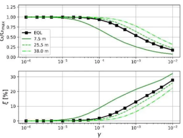
properties are homogeneous along the depth and illustrated in Figure 7. For the fully non-linear approach, 232

the soil mechanical parameters are also shown in Figure 7. Those parameters were chosen as they characterize 233

a typical non-linear soil layer [36]. The non-linear constitutive model implemented defines non-linear 234

properties that depends on the confining pressure and consequently on the considered depth, while Vs 235

remains the same in the whole layer. Figure 7 shows in green the modulus reduction curves and damping 236

curves at different depths. 237

The bedrock is modeled as an infinite monotonic and elastic material with shear velocity of 1500 m/s, a density 238

of 2000 kg/m3_{, and a Poisson coefficient of 0.3. A Gabor wavelet is used as input signal. This simple wavelet}

239

makes easier the evaluation of non-linear effects in the BSR. The Gabor’s wavelet is defined with the Equation 240 (6). 241 _( ) = J `abcde(fgfh)i j b k3 (2l [( − 3)) (6) 242

In the simulations, γ is taken as 3, to as 2.5s. The central frequency (fm=1.25 Hz) is chosen in agreement with

243

the fundamental resonance frequency of the site and only frequencies lower than 2 Hz are analyzed, as the 244

energy of the input signal at higher frequencies is too small to make the ratio computation relevant. A 245

corresponds to the maximal amplitude of the signal. 246

247

Figure 7. Modulus reduction curve and damping curve that are used in: Equivalent Linear approx.

248

(black line-squares), and at different depths for the full non-linear model (green lines). The color

249

version of this figure is available only in the electronic edition.

250 251

For the fully non-linear approach, the soil mechanical parameters are given in Table 1. They were chosen as 252

they characterize a typical non-linear soil layer [36]. In the linear domain, the fundamental resonance 253

frequency of this soil column is equal to 1.25 Hz. 254

Table 1. Parameters of the soil layer for the 1-D numerical simulation.

255 Vs1 _{(m/s) 200} Vp2 _{(m/s) 374} ρ3 _(Kg/m3_{) 1750} Φ4_{(°) 25} β5 ₁₀ σci/σv6 2 Ep7 ₂₀ C8 _{(kPa) 0} γelastic9 1x10-9 b10 _0.9 nr11 _0.4 ψ12_{(°) 20}

1 _{Shear wave velocity (m/s)} 2 _{Primary wave velocity (m/s)} 3 _{Density (Kg/m}3₎

4 _{Friction angle at totally mobilized plasticity (°)} 5 _{Plastic modulus}

6 _{Compaction ratio}

7 _{Plastic stiffness coefficient} 8 _{Cohesion (kPa)}

9 _{Extent of the truly elastic domain} 10 _{Shape parameter of the yield Surface} 11 _{Numerical parameter of isotropic hardening} 12 _{Slope of the characteristic line (°)}

αψ13 0.8

256

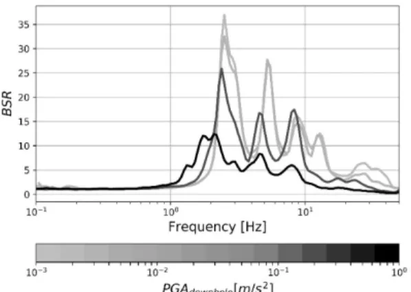
We test different input signal amplitudes and calculate the BSR in each case. The maximum amplitudes of the 257

signals are: 0.001, 0.01, 0.05, 0.1, 0.3, 0.7 and 1 m/s2_{, results are shown in Figure 8. For the smallest PGA, the}

258

computed BSR is equivalent to the analytical elastic case (black dash line). As expected for the larger input 259

motions, the amplification peak is smaller, and it is shifted towards lower frequencies. The equivalent linear 260

computation (Figure 8A) leads to resonance frequency shift larger than the fully non-linear approach (Figure 261

8B). Indeed, besides the limitations of EQL approaches at large strain [37], the non-linear soil properties differ 262

in the two numerical approaches as mentioned above. Indeed, at the soil to bedrock interface, the non-linear 263

soil properties are much more linear in the fully non-linear computation. 264

265

Figure 8. BSR for the equivalent linear approach (a) and the fully non-linear simulation (b) for a

266

different level of input solicitation. Black dash is the elastic response curve.

267

In the linear equivalent approach, the effective strain (γeff) is used to calculate the equivalent shear modulus

268

and damping at each iteration. It is defined from the maximal strain as γeff= 0.65γmax. In Figure 9a, the values

269

of the G/Gmax ratio computed using γeff and γmax are compared to the appropriate fsp values. Taking into

270

account γmax leads to a misfit between fsp and the ratio at high deformation level. Those differences are

271

related to the EQL methodology who computes the non-linear parameters with γeff instead γmax. Considering

272

G/Gmax at yeff, the frequency shift equals almost the shear modulus reduction. The small error can be

273

attributed to the iteration scheme implemented in the linear equivalent method. The good fitting between 274

G/Gmax and fsp curves shows that fsp parameter is able to quantify the amount of shear modulus reduction as

275

equivalent linear method does in this very simple mono-layer case. 276

Figure 9b presents the G/Gmax ratio at different depths in function of the fsp parameter calculated from the

277

BSR curves for a full non-linear approach. The G/Gmax ratio used in these graphs is computed considering the

278

effective strain (γeff) at the middle of the layer for various depths in the non-linear computations (Figure 7).

279

From this figure, we observe that G/Gmax and fsp are not equivalent at all depths in the fully non-linear

280

approach. Indeed, the curves showed on the graph depend on the depth considered for the computation of 281

the shear modulus, as both the non-linear soil properties and the shear strain varies with depth. However, we 282

notice that Equation (5) still can be applied to the curve computed at 25.5 m at depth. At this specific depth, 283

the reason why fsp is not perfectly equal to the G/Gmax ratio on the whole fsp range could be related to the

284

definition of γeff using an approximation of the shear strain during the shaking. At shallower depths, fsp

285

overestimates the shear modulus decrease. On the contrary, at larger depths fsp underestimates slightly the 286

G/Gmax ratio.

287 288

289

Figure 9. Evolution of the shear decay reduction in function of fsp. Left: equivalent linear approach.

290

Right: full non-linear simulation. Red dotted curve: G/Gmax = fsp. The color version of this figure is

291

available only in the electronic edition.

292 293

3.4

Prediction of non-linear surface ground motion using fsp curves

294

In order to go further, we aim to develop a methodology to predict the non-linear surface ground motion 295

using the fsp curves previously computed. For a given site, knowing the PGA value at the downhole sensor, 296

we propose to estimate fsp from the non-linear regression defined in the Equation (3) previously computed 297

at the station. Combining fsp and BSRlinear, it is possible to estimate the BSR for the predicted ground motion.

298

This estimation consists in applying the predicted frequency shift to BSRlinear as shown in Equation (7).

299

m

S

where

m

300

ratio, and fsp, the estimated frequency shift from the hyperbolic curve defined for the site (Equation (3)). 301

We then assume that

m

With this assumption, using

m

motion at the surface : 304

JRn'L&o%= p( ) ∙ JMNO$PN#% (8)

Where Asurface represents the Fourier transform of the accelerogram at the surface, Adownhole is the Fourier

305

transform of the accelerogram at downhole, and

m

Equation (7). 307

4

Results

308

4.1

Application to the whole KiK-net database

309 310

We compute the fsp curves for the 650 considered sites (Figure 10). In order to take into account only the 311

sites where a reliable fsp could be derived, we choose to select the 462 sites having a standard deviation lower 312

than 0.07. On figure 10, the curves are drawn with plain lines in the PGA range covered by the data and are 313

represented with dashed lines in the PGA range where the curve is extrapolated. At some sites, the curve is 314

linear over the whole PGA domain, meaning that there is no shift of frequency no matters the intensity of the 315

ground motion is. In other sites, the decrease of fsp starts at low PGA, meaning that even for weak motions a 316

shift of the peak frequencies is significant. The variability of the curves reflects the variability of the non-linear 317

soil behavior at the different sites. The figure shows as well, that for some PGA at the downhole, all of the 318

sites are prone to develop non-linear soil behavior. For example, for the evaluated stations in this study, 50% 319

of the stations have an fsp lower than 0.8 for a PGAdownhole of 4.4x10-1 m/s2. 25% have developed a lower value

320

of fsp for a PGAdownhole of 2.3 x10-1 m/s2, and 75% for PGAdownhole of 8.4x10-1 m/s2.

321

322

Figure 10. fsp curves for 462 sites of the Kik-Net network. Continuous lines indicate that the curves

323

are interpolated using data, dash lines indicate the portion of curves that are extrapolated. Orange

324

line data is shown in Figure 11. The color version of this figure is available only in the electronic

325

edition.

326

Among all of the KiK-net sites, we performed a selection of 8 sites to show in more details the fsp curves. We 327

select sites with different range of PGArefdownhole and sites that have recorded very large earthquakes as

328

Fukushima or Kumamoto earthquakes. The fsp curves derived at these stations are already shown in orange 329

in Figure 10. They are presented in Figure 11 together with the individual fsp obtained for each recorded 330

earthquake. In this figure, the graphs are organized from very non-linear stations to linear ones. The Table 2 331

shows the PGArefdownhole, the Vs30, and the depth where the downhole station is located.

333

Figure 11. fsp curve for several stations that represents the general behavior of the data set. The

334

blue line is the hyperbolic function that is fitted in each case. The color version of this figure is

335

available only in the electronic edition.

336

Table 2. General data for 10 selected sites.

337 Station Name PGArefdownhole [m/s2_] Vs30 [m/s] Depth [m] HRSH13 3.08E-01 399 200 IWTH21 5.03E-01 521 100 IBRH16 7.05E-01 626 300 AKTH16 1.45E+00 375 154

YMTH02 3.55E+00 279 150 YMTH01 4.95E+00 328 207 MYGH08 1.00E+01 203 100 AICH04 ∞ 241 1055 338

PGArefdownhole is the parameter that quantifies the susceptibility of a site to show a non-linear behavior. The

339

higher it is, the less non-linear the site is. We can observe that the variation between stations is significant. 340

The PGArefdownhole go from 3.1x10 -1 m/s2 for the station HRSH13 to infinite for AICH04. The hyperbolic trend

341

previously describe is well suited for the fsp distribution in function of PGAdownhole at almost all of the stations.

342

However, we can note that at station IWTH21, the hyperbolic model (blue line) is not necessarily the function 343

that would produce the best fit. 344

In Table 2, we conclude that the higher Vs30 is, the smaller PGArefdownhole is, meaning that larger non-linear

345

behavior is observed for site characterized by high Vs30. This has already been reported in previous papers 346

(e.g. Régnier et al., 2014 [7]) with the conclusion that high Vs30 sites, composed of a thin soft soil over a stiff 347

shallow bedrock, create a very large impedance contrast that can induce strong amplification and large strain 348

in the superficial layer during earthquakes. 349

350

4.2

Application to 2016 Kumamoto earthquake recordings, Mw 7.1

351 352

We apply our methodology to the Kumamoto Earthquake recordings. The earthquake mainshock occurred 353

April 15th, 2016 in the south of Japan (island of Kyushu), with a magnitude Mw of 7.0. This earthquake initially 354

started on a deep portion of the northern part of the Hinagu fault and then finished in the Futagawa fault [38], 355

it was the largest earthquake in Japan in 2016. In this section, the recorded ground motions at KIK-net sites 356

(FKOH03, OITH11, and KMMH03) are compared to predicted ones using the methodology described 357

previously. Figure 12 gives the location of the three sites in the Island of Kyushu, the location of the fault and 358

the epicenter according to Yagi et al., (2016). Station FKOH03 is located at 91 km of the fault located in Umi 359

Fukuoka prefecture, with a Vs30 of 497 m/s (site EC8 type C). The bedrock is reached at 25m depth with a Vs

360

of 2030 m/s and the downhole station is located at 100m depth. Station OITH11 is located at 72 km from the 361

epicenter in Kokonoe Oita prefecture. It has been characterized with a Vs30 of 458 m/s (site EC8 type C) and

362

the S wave velocity reaches 800 m/s starting from 65m depth, the downhole station is located at 160 m depth 363

with a Vs of 1000m/s. Finally, KMMH03 is located in the prefecture of Kumamoto in Kikuchi at 27.7 km from 364

the epicenter. Like the two other sites, it is a EC8 type C class with a Vs30 of 421 m/s. The bedrock was found

365

at 80m with a Vs of 1200 m/s and the downhole station is located at 200m depth where Vs of reaches 366

2000m/s. 367

368

Figure 12. Island of Kyushu Japan with the location of the studied stations. The line and the star

369

represent the location of the active fault and the epicenter for Kumamoto earthquake 15th _{April 2016}

370

[39].

371

372

Figure 13. Vs profiles of evaluated sites for the earthquake of Kumamoto 2016. (a) site FKOH03. (b)

373

site OITH11. (c) site KMMH03.

374

We compute the fsp curves for the three sites (Figure 14) using 140, 57, and 111 earthquakes for station 375

FKOH03, OITH11, and KMMH03 respectively leaving on the side the recordings of the main Kumamoto event. 376

On figure 14, we report together with the fsp curves, the PGA values at downhole recorded during the 377

Kumamoto earthquake (orange vertical line). We note that the ground motions recorded during this event 378

were larger than all the other events of the database for stations OITH11 and KMMH03. Therefore, for these 379

stations, fsp is estimated by extrapolation of the fsp curves calculated on weaker motions. The performance 380

of the extrapolation depends on the site and the available data. If no large or medium earthquakes have been 381

recorded at a site, the non-linear regression is not well constrained at larger PGA and the estimated shift will 382

be assorted with important uncertainties. On the contrary, at FKOH03, the fsp is assessed by interpolation 383

leading to a better confidence. However, even here, the dispersion between the curve and the real data 384

remains. 385

386

Figure 14. fsp parameter in function of the PGAdownhole. (a) site FKOH03. (b) site OITH11. (c) site

387

KMMH03. The vertical line represents the PGAdownhole generated by the Kumamoto 2016 earthquake

388

at each site.

389

The p derived from the BSRlinear with the predicted frequency shift are illustrated in Figure 15 in black thick

390

lines along with the observed BSR in grey lines and the linear BSR in dotted line. For the three cases, the 391

estimated p is closer to the observed BSR than to the linear BSR. This result shows that the shift correction 392

we propose is relevant for large ground motions, when the nonlinear soil behavior is running. Furthermore, 393

we observe that the shift in the BSR is well predicted even with an extrapolated fsp. 394

At station FKOH03 that experienced the weaker motion during this earthquake (PGAdownhole ~ 0.2 m/s2), the

395

correction on BSRlinear is very small and do not particularly change the frequency content of the motion. But

396

at station OITH11, that recorded a larger PGAdownhole (about 2m/s2), the correction is important leading in a

397

prediction fiting very well the real surface data. On this station, the BSR has one main peak and a simple shape. 398

Station KMMH03 also recorded a strong PGAdownhole but its BSR is more complex, with various peak frequencies

399

(mainly two around 1Hz and 10Hz) over a large frequency band. This station is located within few kilometers 400

of the active fault. Consequently, it is subject to near-source high frequency effects. The correction applied is 401

very efficient on the lower frequency of the BSR but tends to shift a little too much the higher frequency part 402

(> 10z). For this station, we observe that the shift shouldn’t be the same for all frequencies. This could be due 403

to others causes than the non-linear soil behavior alone. 404

405

Figure 15. Comparison between the BSRlinear for each site (black dashed line) computed on weak

406

motion, the BSR computed on the Kumamoto earthquake recordings (orange line), and the

407

correction of the borehole transfer function (qrs

m

408

(b) site OITH11. (c) site KMMH03. The color version of this figure is available only in the electronic

409

edition.

410

Table 3 illustrates the improvement offered by the proposed methodology in the predicting of strong ground 411

motion. We compute the difference in frequency of the BSR peaks between the observation and the related 412

prediction. From this table, it is clear that the differences are lower when the BSR is corrected by the fsp shift. 413

Indeed, at OITH11 and KMMH03, the methodology improves the prediction of the frequency peak by around 414

50%. At FKOH03, the ground motion was not strong enough to show some non-linear soil behavior during the 415

main event. However, even in this case, we can see that a little improvement is provided by our approach. 416

Table 3. Relative comparison between the main peak frequencies in the observed BSR, the estimated

417 BSR, and BSRlinear. 418 FKOH03 OITH11 KMMH03 BSRObserved to p 2% 8% 2% BSRObserved to BSRlinear 15% 58% 50% 419

The Fourier spectrum for the geometric average of the horizontal components is computed according to the 420

Equation (1). The results are presented in Figure 16 for the three sites on which we are focusing here. 421

422

Figure 16. Fourier spectrum at the surface of the horizontal components. Earthquake of Kumamoto

423

15th _{April. (a) site FKOH03. (b) site OITH11. (c) site KMMH03. The color version of this figure is}

424

available only in the electronic edition.

The predictions of the surface ground motion are improved when the site response is corrected by the 426

adequate frequency shift. Comparing the main peaks frequency position of the Fourier spectra at the surface, 427

Table 4 shows the relative difference between observations and predictions. In the case of the site FKOH03, 428

the difference is small since the target ground motion isn’t strong enough to exhibit a non-linear behavior of 429

the soil. But even in this case, the spectra obtained with the fsp correction is closer to the observed spectra. 430

For the two other sites, the prediction of the main peak frequency position is improved by more than 40% in 431

both cases in comparison with the direct use of BSRlinear.

432

Table 4. Comparison of the main peaks in the spectra at the surface between the observation and

433

the computed spectra using qrsp and BSRlinear.

434

FKOH03 OITH11 KMMH03 Asurface to p ·Adownhole 4% 8% 0% Asurface to BSRlinear· Adownhole 10% 60% 44%

5

Discussion

435 436

To estimate precisely the ground motion at the surface in the time domain, an inverse Fourier transform 437

should be applied to the estimation of the Fourier spectrum. Additionally, the same previously described 438

process should be applied independently for each horizontal components of then ground motion. However, 439

the phase modification due to the site effects should also be taken into account. This effect has been studied 440

before, and usually, it is assumed that 1D site effect does not modify consequently the phase [40]. Since we 441

are using borehole arrays configuration, the applicability of the same assumptions must be evaluated, and it 442

will be part of future studies. 443

The application of the parameter fsp is very promising for the prediction of the non-linear ground motion. In 444

a simple case, we demonstrate that the parameter fsp provides a good evaluation of the shear modulus 445

reduction. In a full non-linear approach, the parameter provides an average quantification of the decrease of 446

the shear modulus. For both cases, the parameter gives a good quantification of the impact of the non-linear 447

soil behavior in the site response. 448

For now, the definition of the fsp parameter requires a vertical array of accelerometers and weak to moderate 449

earthquake recordings to define the fsp curves. To overpass this limitation, we are currently working on the 450

prediction of the fsp curves at non-instrumented sites but characterized by specific geotechnical parameters 451

as Vs30 and f0 that has been demonstrated to be a good proxy parameter for describing the potential

non-452

linear site behavior of a site (e.g. [10] Régnier et al 2016). To predict the rock motion at the downhole station 453

(with the effects of the down-going waves) several methods could be applied such as the Empirical Green’s 454

Function directly at downhole or with a correction method to transfer from surface to borehole as proposed 455

in Cadet et al. [41] or the use of numerical models. 456

6

Conclusions

457 458

We propose in this paper to quantify the effects of non-linear site behavior by measuring the frequency shift 459

that it produces in the Borehole Spectral Ratio (BSR) from weak motion to stronger one. The logarithmic shift 460

of BSR, that we called frequency shift parameter (fsp), is related to the intensity of the ground motion. For 461

each site, we, therefore, defined fsp curves that relate the fsp parameter to the PGA at the downhole station 462

following the classic hyperbolic model. We thus are able to estimate the non-linear effects of strong ground 463

motions at sites using enough recorded data. 464

We showed that the frequency shift parameter (fsp) is a good proxy for non-linear site behavior, as the fsp 465

curves could mimic the shear modulus reduction curves. This fitting is better accomplished when an 466

appropriate parameter to approximate the shear strain in the soil column during the shaking is used. 467

For the earthquake of Kumamoto 2016, we estimated the non-linear site response and the Fourier spectrum 468

at the surface, including the non-linear effects based on the linear site response and the corresponding rock 469

downhole recording of the earthquake. The prediction provided very close results to the observations and, 470

for sites with high nonlinearity, it improves in our case by more than 40% the frequency position of the main 471

peak compared to a linear evaluation. The fsp curves provide, as shear modulus reduction curves do, an 472

evaluation of the propensity of a site to develop non-linearity as well a possible way to quantify the level of 473

non-linearity of the site under strong earthquakes. 474

Acknowledgments

475

All authors are thankful with the National Research Institute for Earth Science and Disaster Resilience (NIED) 476

in Japan for making Kik-net data available and collected the used data in this paper. Those data can be 477

obtained from web site www.kyoshin.bosai.go.jp (last accessed October 2017). 478

We are thankful to the anonymous reviewers for their fruitful comments that improved the manuscript. 479

Also, we thank the professor Fernando Lopez Caballero from Centrale Supelec, Paris-Saclay France, for his 480

help to interpret the CyberQuake analysis. 481

The data in this study for any station and ground motion (e.g. fsp, PGA, PGV) are available upon request. 482

Bibliography

483

[1] Bard P-Y, Bouchon M. The two-dimensional resonance of sediment-filled valleys. Bull Seismol Soc Am 484

1985;75:519–41. 485

[2] Cranswick E, King K, Carver D, Worley D, Williams R, Spudich P, et al. Site response across downtown 486

Santa Cruz, California. Geophys Res Lett 1990;17:1793–6. 487

[3] Lermo J, Chavez-Garcia FJ. Site effect evaluation using spectral ratios with only one station. Bull Seismol 488

Soc Am 1993;83:1574–94. 489

[4] Kramer L. Geotechnical earthquake engineering. vol. 1. Prentice-Hall International Series; 1996. 490

[5] Thompson EM, Baise LG, Kayen RE, Guzina BB. Impediments to Predicting Site Response: Seismic 491

Property Estimation and Modeling Simplifications. Bull Seismol Soc Am 2009;99:2927–49. 492

doi:10.1785/0120080224. 493

[6] Rubinstein JL. Nonlinear Site Response in Medium Magnitude Earthquakes near Parkfield, 494

CaliforniaNonlinear Site Response in Medium Magnitude Earthquakes near Parkfield, California. Bull 495

Seismol Soc Am 2011;101:275–86. doi:10.1785/0120090396. 496

[7] Régnier J, Cadet H, Bonilla LF, Bertrand E, Semblat J-F. Assessing Nonlinear Behavior of Soils in Seismic 497

Site Response: Statistical Analysis on KiK-net Strong-Motion Data. Bull Seismol Soc Am 2013;103:1750– 498

70. doi:10.1785/0120120240. 499

[8] Zeghal M, Elgamal A. Analysis of Site Liquefaction Using Earthquake Records. J Geotech Eng 500

1994;120:996–1017. doi:10.1061/(ASCE)0733-9410(1994)120:6(996). 501

[9] Assimaki D, Li W, Steidl J, Schmedes J. Quantifying Nonlinearity Susceptibility via Site-Response 502

Modeling Uncertainty at Three Sites in the Los Angeles Basin. Bull Seismol Soc Am 2008;98:2364–90. 503

doi:10.1785/0120080031. 504

[10] Régnier J, Cadet H, Bard P-Y. Empirical Quantification of the Impact of Nonlinear Soil Behavior on Site 505

Response. Bull Seismol Soc Am 2016;106:1710–9. 506

[11] Bonilla LF, Archuleta RJ, Lavallée D. Hysteretic and Dilatant Behavior of Cohesionless Soils and Their 507

Effects on Nonlinear Site Response: Field Data Observations and Modeling. Bull Seismol Soc Am 508

2005;95:2373–95. doi:10.1785/0120040128. 509

[12] Pavlenko OV. Possible Mechanisms for Generation of Anomalously High PGA During the 2011 Tohoku 510

Earthquake. Pure Appl Geophys 2017;174:2909–24. doi:10.1007/s00024-017-1558-2. 511

[13] Aguirre J, Irikura K. Nonlinearity, liquefaction, and velocity variation of soft soil layers in Port Island, 512

Kobe, during the Hyogo-ken Nanbu earthquake. Bull Seismol Soc Am 1997;87:1244–58. 513

[14] Iai S, Morita T, Kameoka T, Matsunaga Y, Abiko K. Response of a Dense Sand Deposit during 1993 514

Kushiro-Oki Earthquake. Soils Found 1995;35:115–31. doi:10.3208/sandf1972.35.115. 515

[15] Wen K-L. Non-linear soil response in ground motions. Earthq Eng Struct Dyn 1994;23:599–608. 516

doi:10.1002/eqe.4290230603. 517

[16] Ishibashi I, Zhang X. Unified dynamic shear moduli and damping ratios of sand and clay. SOILS Found 518

1993;33:182–91. doi:10.3208/sandf1972.33.182. 519

[17] Vucetic Mladen. Cyclic Threshold Shear Strains in Soils. J Geotech Eng 1994;120:2208–28. 520

doi:10.1061/(ASCE)0733-9410(1994)120:12(2208). 521

[18] Zeghal M, Elgamal AW, Tang HT. Lotung Downhole Array. II: Evaluation of Soil Nonlinear Properties | 522

Journal of Geotechnical Engineering | Vol 121, No 4. J Geotech Eng 1995;121. doi:10.1061/(ASCE)0733-523

9410(1995)121:4(363). 524

[19] Glaser S, Baise L. System identification estimation of soil properties at the Lotung site - ScienceDirect. 525

Soil Dyn Earthq Eng 2000;19:521–31. doi:10.1016/S0267-7261(00)00026-9. 526

[20] Pavlenko OV, Irikura K. Estimation of Nonlinear Time-dependent Soil Behavior in Strong Ground Motion 527

Based on Vertical Array Data. Pure Appl Geophys 2003;160:2365–79. doi:10.1007/s00024-003-2398-9. 528

[21] Nakata N, Snieder R. Estimating near-surface shear wave velocities in Japan by applying seismic 529

interferometry to KiK-net data. J Geophys Res Solid Earth 2012;117. doi:10.1029/2011JB008595. 530

[22] Bonilla LF, Guéguen P, Lopez-Caballero F, Mercerat ED, Gélis C. Prediction of non-linear site response 531

using downhole array data and numerical modeling: The Belleplaine (Guadeloupe) case study. Phys 532

Chem Earth Parts ABC 2017;98:107–18. doi:10.1016/j.pce.2017.02.017. 533

[23] Noguchi S, Sasatani T. Quantification of degree of nonlinear site response, 2008, p. 0049. 534

[24] Lussou P, Bard P-Y, Modaressi H, Gariel J-C. Quantification of soil non-linearity based on simulation. Soil 535

Dyn Earthq Eng 2000;20:509–16. doi:10.1016/S0267-7261(00)00100-7. 536

[25] Field EH, Johnson PA, Beresnev IA, Zeng Y. Nonlinear ground-motion amplification by sediments during 537

the 1994 Northridge earthquake. Nature 1997;390:599–602. doi:10.1038/37586. 538

[26] Boore DM. On Pads and Filters: Processing Strong-Motion Data. Bull Seismol Soc Am 2005;95:745–50. 539

doi:10.1785/0120040160. 540

[27] Oppenheim AV, Schafer RW. Discrete-time signal processing. Pearson Higher Education; 2010. 541

[28] Konno K, Ohmachi T. Ground-motion characteristics estimated from spectral ratio between horizontal 542

and vertical components of microtremor. Bull Seismol Soc Am 1998;88:228–41. 543

[29] Field EH, Jacob KH. A comparison and test of various site-response estimation techniques, including 544

three that are not reference-site dependent. Bull Seismol Soc Am 1995;85:1127–43. 545

[30] Régnier J, Bonilla L-F, Bard P-Y, Bertrand E, Hollender F, Kawase H, et al. PRENOLIN: International 546

Benchmark on 1D Nonlinear Site-Response Analysis—Validation Phase Exercise. Bull Seismol Soc Am 547

2018. 548

[31] Duncan J, Chang C. Nonlinear analysis of stress and strain in soils. ASCE J Soil Mech Found 1970;96:1629– 549

53. 550

[32] Ishihara K. Soil Behaviour in Earthquake Geotechnics. Oxford: Clarenton Press; 1996. 551

[33] Chandra J, Guéguen P, Bonilla LF. PGA-PGV/Vs considered as a stress–strain proxy for predicting 552

nonlinear soil response. Soil Dyn Earthq Eng 2016;85:146–60. doi:10.1016/j.soildyn.2016.03.020. 553

[34] Modaressi H, Foerster E. CyberQuake. User’s Man BRGM Fr 2000. 554

[35] Hujeux J. Une loi de comportement pour le chargement cyclique des sols. Génie Parasismique 555

1985:287–302. 556

[36] Lopez-Caballero F, Modaressi-Farahmand-Razavi A, Modaressi H. Nonlinear numerical method for 557

earthquake site response analysis I — elastoplastic cyclic model and parameter identification strategy. 558

Bull Earthq Eng 2007;5:303–23. doi:10.1007/s10518-007-9032-7. 559

[37] Kaklamanos J, Bradley BA, Thompson EM, Baise LG. Critical Parameters Affecting Bias and Variability in 560

Site-Response Analyses Using KiK-net Downhole Array DataCritical Parameters Affecting Bias and 561

Variability in Site-Response Analyses. Bull Seismol Soc Am 2013;103:1733–49. 562

doi:10.1785/0120120166. 563

[38] Asano K, Iwata T. Source rupture processes of the foreshock and mainshock in the 2016 Kumamoto 564

earthquake sequence estimated from the kinematic waveform inversion of strong motion data. Earth 565

Planets Space 2016;68:147. doi:10.1186/s40623-016-0519-9. 566

[39] Yagi Y, Okuwaki R, Enescu B, Kasahara A, Miyakawa A, Otsubo M. Rupture process of the 2016 567

Kumamoto earthquake in relation to the thermal structure around Aso volcano. Earth Planets Space 568

2016;68:118. doi:10.1186/s40623-016-0492-3. 569

[40] Fleur SS, Bertrand E, Courboulex F, Lépinay BM de, Deschamps A, Hough S, et al. Site Effects in Port-au-570

Prince (Haiti) from the Analysis of Spectral Ratio and Numerical Simulations. Bull Seismol Soc Am 2016. 571

doi:10.1785/0120150238. 572

[41] Cadet H, Bard P-Y, Rodriguez-Marek A. Site effect assessment using KiK-net data: Part 1. A simple 573

correction procedure for surface/downhole spectral ratios. Bull Earthq Eng 2012;10:421–48. 574

doi:10.1007/s10518-011-9283-1. 575