HAL Id: hal-01650998
https://hal.archives-ouvertes.fr/hal-01650998
Submitted on 11 Jan 2018
HAL is a multi-disciplinary open access
archive for the deposit and dissemination of
sci-entific research documents, whether they are
pub-lished or not. The documents may come from
teaching and research institutions in France or
abroad, or from public or private research centers.
L’archive ouverte pluridisciplinaire HAL, est
destinée au dépôt et à la diffusion de documents
scientifiques de niveau recherche, publiés ou non,
émanant des établissements d’enseignement et de
recherche français ou étrangers, des laboratoires
publics ou privés.
Extensibility and Composability of a Multi-Stencil
Domain Specific Framework
Hélène Coullon, Julien Bigot, Christian Pérez
To cite this version:
Hélène Coullon, Julien Bigot, Christian Pérez. Extensibility and Composability of a Multi-Stencil
Domain Specific Framework. International Journal of Parallel Programming, Springer Verlag, 2017,
�10.1007/s10766-017-0539-5�. �hal-01650998�
(will be inserted by the editor)
Extensibility and Composability of a Multi-Stencil
Domain Specific Framework
H´el`ene Coullon · Julien Bigot · Christian Perez
the date of receipt and acceptance should be inserted later
Abstract As the computation power of modern high performance architec-tures increases, their heterogeneity and complexity also become more impor-tant. One of the big challenges of exascale is to reach programming models that give access to high performance computing (HPC) to many scientists and not only to a few HPC specialists. One relevant solution to ease parallel program-ming for scientists is Domain Specific Language (DSL). However, one problem to avoid with DSLs is to mutualize existing codes and libraries instead of im-plementing each solution from scratch. For example, this phenomenon occurs for stencil-based numerical simulations, for which a large number of languages has been proposed without code reuse between them. The Multi-Stencil Frame-work (MSF) presented in this paper combines a new DSL to component-based programming models to enhance code reuse and separation of concerns in the specific case of stencils. MSF can easily choose one parallelization technique or another, one optimization or another, as well as one back-end implemen-tation or another. It is shown that MSF can reach same performances than a non component-based MPI implementation over 16.384 cores. Finally, the performance model of the framework for hybrid parallelization is validated by evaluations.
H´el`ene Coullon
DAPI IMT Atlantique, LS2N, Inria. Nantes, France E-mail: [email protected]
Julien Bigot
Maison de la Simulation, CEA, CNRS, Univ. Paris-Sud, UVSQ, Universit´e Paris-Saclay, 91191 Gif-sur-Yvette, France
E-mail: [email protected] Christian Perez
Univ. Lyon, Inria, CNRS, ENS de Lyon. Lyon, France E-mail: [email protected]
Keywords Component programming models · Domain Specific Language (DSL) · Stencil · Numerical simulation · Data parallelism · Task parallelism · Scheduling · MPI · OpenMP
1 Introduction
As the computation power of modern high performance architectures increases, their heterogeneity and complexity also become more important. For example, the current fastest supercomputer Tianhe-21is composed of multi-cores pro-cessors and accelerators, and is able to reach a theoretical peak performance of about thirty peta-flops (floating-point operations per second). However, to be able to use such machines, multiple programming models, such as MPI (Message Passing Interface), OpenMP, CUDA, etc., and multiple optimiza-tion techniques, such as cache optimizaoptimiza-tion, have to be combined. Moreover, current architectures evolution seems to indicate that heterogeneity and com-plexity in HPC will continue to grow in the future.
One of the big challenges to be able to use those upcoming Exascale com-puters is to propose programming models that give access to high performance computing (HPC) to many scientists and not only to a few HPC specialists [15]. Actually, applications that run on supercomputers and need such computa-tion power (e.g. physics, weather or genomic) are typically not implemented by HPC specialists but by domain scientists.
Many general purpose languages and frameworks have improved the sim-plicity of writing parallel codes. For example PGAS models [23] or task-based frameworks, such as OpenMP [13], Legion [4] or StarPU [2], partially hide intricate details of parallelism to the user. For non-expert users however, these languages and frameworks are still difficult to use. Moreover, tuning an ap-plication for a given architecture is still very complex to achieve with these solutions. An interesting approach that combines simplicity of use, due to a high abstraction level, with efficient execution are domain specific languages (DSL) and domain specific frameworks (DSF). These solutions are specific to a given domain and propose a grammar or an API which is easy to understand for specialists of this domain. Moreover, knowledge about the targeted domain can be embedded in the compiler that can thus automatically apply paralleliza-tion and optimizaparalleliza-tion techniques to produce high performance code. Domain specific solutions are therefore able to separate end-user concerns from HPC concerns which is a requirement to make HPC accessible to a wider audience. Many domain specific languages and frameworks have been proposed. Each one claims to handle a distinct specific optimization or use case. Each solution is however typically re-implemented from scratch. In this paper, we claim that the sharing of common building blocks when designing DSLs or DSFs would in-creases re-use, flexibility and maintainability in their implementation. It would also ease the creation of approaches and applications combining multiple DSLs and DSFs.
For example, some of the approaches to numerically solve partial differen-tial equations (PDEs) lead to stencil computations where the values associated to one point in space at a given time are computed from the values at the pre-vious time at the exact same location together with a few neighbor locations. Many DSLs have been proposed for stencil computations [7, 8, 14, 26, 30] as detailed in Section 7. Many of them use the same kind of parallelization, data structures or optimization techniques, however each one has been built from scratch.
We propose the Multi-Stencil Framework (MSF) that is built upon a meta-formalism of multi-stencil simulations. MSF produces a parallel orchestration of a multi-stencil program without being aware of the underlying implementa-tion choices (e.g., distributed data structures, task scheduler etc.). Thanks to this meta-formalism MSF is able to easily switch from one parallelization tech-nique to another and from one optimization to another. Moreover, as MSF is independent from implementation details, MSF can easily choose one back-end or another, thus easing code reuse of existing solutions. To ease composition of existing solutions, MSF is based on component-based programming [29], where applications are defined as an assembly of building blocks, or components.
After a short overview of the Multi-Stencil Framework given in Section 2, the paper is organized as follows. The meta-formalism of a multi-stencil pro-gram is presented in Section 3; from this formalism are built both a light and descriptive domain specific language, namely MSL, as well as a generic com-ponent assembly of the application both described in Section 4; the compiler of the framework is described in Section 5; finally a performance evaluation is detailed in Section 6 .
2 The Component-Based Multi-Stencil Framework
This section first presents a background on component models and particularly on the Low Level Components. This background is needed to understand the second part of the section which gives an overview of the overall Multi-Stencil Framework (MSF).
2.1 Background on component models
Component-based software engineering (CBSE) is a domain of software en-gineering [29] which aims at improving code re-use, separations of concerns, and thus maintainability. A component-based application is made of a set of component instances linked together, this is also called a component assembly. A component is a black box that implements an independent functionality of the application, and which interacts with its environment only through well defined interfaces: its ports. For example, a port can specify services provided or required by the component. With respect to high performance computing, some works have also shown that component models can achieve the needed
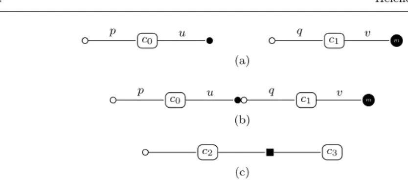
c0 c1 m p u q v (a) c0 c1 m p u q v (b) c2 c3 (c)
Fig. 1: Example of components and their ports representation. a) Component c0 has a provide port (p) and a use port (u); Component c1has also a provide port (q) but also a use multiple port (v). b) A use port is connected to a (com-patible) provide port. c) Component c2and c3 shares an MPI communicator.
level of performance and scalability while also helping in application portabil-ity [1, 6, 27].
Many component models exist, each of them with its own specificities. Well known component models include, for example, the CORBA Component Model (CCM) [24], and the Grid Component Model (GCM) [3] for distributed computing, while the Common Component Architecture (CCA) [1], and Low Level Components (L2C) [5] are HPC-oriented. This work makes use of L2C for the experiments.
L2C [5] is a minimalist C++ based HPC-oriented component model where a component extends the concept of class. The services offered by the compo-nents are specified trough provide ports, those used either by use ports for a single service instance, or use − multiple ports for multiple services instances. Services are specified as C++ interfaces. L2C also offers M P I ports that enable components to share MPI communicators. Finally, components can also have attribute ports to be configured. In this paper, and as illustrated in Figure 1, a provide port is represented by a white circle, a use port by a black circle, a use − multiple port by a black circle with a white m in it. MPI port are connected with a black rectangle. A L2C-based application is a static assem-bly of components instances and the connections between their ports. Such an assembly is described in LAD, an XML dialect, and is managed by the L2C runtime system that minimize overheads by loading simple dynamic libraries. One can also notice that L2C can achieve performance if the granularity of components is high enough and attentively chosen by the user. The typical overhead of a L2C is a C++ indirect virtual method invocation.
2.2 Multi-Stencil Framework overview
The Multi-Stencil Framework helps end-users to produce high performance parallel applications for the specific case of multi-stencils. The multi-stencil
Numerician Generic Assembly Multi-Stencil Language Multi-Stencil Compiler Specialized assembly HPC spec. Developer Multi-St encil Fr amework +
Fig. 2: The Multi-Stencil Framework (MSF) is composed of the Multi-Stencil Language (MSL), the Generic Assembly (GA) and the Multi-Stencil Compiler (MSC) to produce a specialized assembly of components. The numerician, or mathematician uses MSL to describe its simulation. The developer will imple-ment components responsible for numerical codes. A third party HPC special-ist can interact with MSF to propose different version of HPC components.
domain will be formally defined in the next section. A multi-stencil program numerically solves PDEs using computations that can use neighborhood values around an element, also called a stencil computation.
Figure 2 gives an overview of the Multi-Stencil Framework that is entirely detailed throughout this paper. It is composed of four distinct parts described hereafter. As illustrated in Figure 2, MSF targets two different kinds of end-users: the numerician, in other words the mathematician, and the developer. Most of the time numericians do have programming knowledge, however as it is not their core domain and because of a lack of time, development is often left to engineers according to numerician needs. MSF has the interesting particularity to propose a clear separation of concerns between these two end-users by distinguishing the description of the simulation from the implementation of numerical codes.
MSF also has the interesting capability to be more flexible than existing solutions thanks to a possibility for a third party to interact with the frame-work. This third party is a High Performance Computing (HPC) specialist as displayed in Figure 2.
Multi-Stencil Language The Multi-Stencil Language, or MSL, is the do-main specific language proposed by the framework for the numerician. It is a descriptive language, easy to use, without any concern about implementation details. It fits the need of a mathematician to describe the simulation. The description written with MSL can be considered as an input of the frame-work. MSL is described in details in Section 4. The language is built upon the formalism described in Section 3.
Generic Assembly In addition to the language MSL, used by the numeri-cian to describe its simulation, MSF needs a Generic Assembly (GA) of a
multi-stencil program as input. What is called a GA is a component assembly for which meta-types of components are represented and for which some parts need to be generated or specialized. A GA could be compared respectively to a template or a skeleton in object programming languages (such as C++) or functional languages. From this generic assembly will be built the final special-ized assembly of the simulation where component types will be specified, and where parts of GA will be transformed. As well as MSL, this generic assembly is described in Section 4 and is built upon the meta-formalism described in Section 3.
Multi-Stencil Compiler The core of the framework is the Multi-Stencil Compiler, or MSC. It is responsible for transforming the generic assembly into the final parallel assembly which is specific to the simulation described by the numerician with MSL. MSC is described in Section 5.
Specialized assembly Finally, the output of MSF is the component assembly generated by MSC. It is an instantiation and a transformation of the generic component assembly, by adding component types, transforming some part of the assembly, and by adding specific components generated by MSC. From this final component assembly which is specific to the simulation initially described with MSL, the developer will finally write components associated to numerical codes, or directly re-use existing components from other simulations. This final specialized component assembly is a parallel orchestration of the computations of the simulation initially described by the numerician. Finally, the specialized assembly produced by MSF is written in L2C.
3 Formalism of a Multi-Stencil Program
The numerical solving of partial differential equations relies on the discretiza-tion of the continuous time and space domains. Computadiscretiza-tions are typically iteratively (time discretization) applied onto a mesh (space discretization). While the computations can have various forms, many direct methods can be expressed using three categories only: stencil computations involve access to neighbor values only (the concept of neighborhood depending on the space dis-cretization used); local computations depend on the computed location only (this can be seen as a stencil of size one); finally, reductions enable to transform variables mapped on the mesh to a single scalar value.
This section gives a complete formal description of what we call a multi-stencil program and its computations. This formalism is general enough to be common to any existing solution already proposed for stencil computations. As a result it can be considered as a meta-formalism or a meta-model of a Multi-Stencil Program. This meta-formalism will be used to define MSL and GA in the next section.
3.1 Time, mesh and data
Let us introduce some notations. Ω is the continuous space domain of a nu-merical simulation (typically Rn). A mesh M defines the discretization of the continuous space domain Ω and is defined as follows.
Definition 1 A mesh is a connected undirected graph M = (V, E), where V ⊂ Ω is the (finite) set of vertices and E ⊆ V2 the set of edges. The set of edges E of a mesh M = (V, E) does not contain bridges. It is said that the mesh is applied onto Ω.
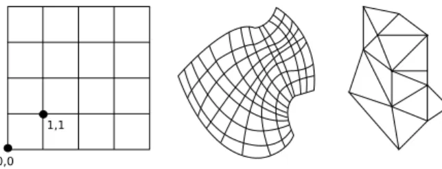
0,0 1,1
Fig. 3: From left to right, Cartesian, curvilinear and unstructured meshes.
A mesh can be structured (as Cartesian or curvilinear meshes), unstructured, regular or irregular (without the same topology for each element) as illustrated in Figure 3.
Definitions (mesh)
– An entity φ of a mesh M = (V, E) is defined as a subset of its vertices and edges, φ ⊂ V ∪ E.
– A group of mesh entities G ∈ P(V ∪ E) represents a set of entities of the same topology.
– The set of all groups of mesh entities used in a simulation is denoted Φ. For example, in a 2D Cartesian mesh, an entity could be a cell, made up of four vertices and four edges. A group of entities could contain all the cells, another would for example contain the vertical edges at the frontier between cells. Both groups would be part of Φ. This example is illustrated in Figure 4a. Definition 2 The finite sequence T : (tn)n∈J0,TmaxK represents the discretiza-tion of the continuous time domain T = R.
The time discretization can be as simple as a constant time-step with a fixed number of steps. The time-step and the number of steps can also change on the fly during execution.
– ∆ are the mesh variables. A mesh variable δ ∈ ∆ associates to each couple entity and time-step a value δ : G × T 7→ Vδ where Vδ is a value type. – The group of entities a variable is mapped on is denoted entity(δ) = G. – S are the scalar variables. A scalar variable s ∈ S associates to each
time-step a value s : T 7→ Vδ where Vδ is a value type. – V = ∆ ∪ S is the set of variables or quantities.
– Among the scalar variables is one specific boolean variable conv ∈ S, the convergence criteria, whose value is 0 except at the last step where it is 1. This scalar can be updated on the fly according to other variables, typically by using a reduction as detailed later.
3.2 Computations
Definitions
– A computation domain D is a subpart of a group of mesh entities, D ⊆ G ∈ Φ.
– The set of computation domains of a numerical simulation is denoted D. – N is the set of neighborhood functions n : Gi 7→ Gjm which for a given
entity φ ∈ Gi returns a set of m entities in Gj. One can notice that i = j is possible. Most of the time, such a neighborhood is called a stencil shape. Definition 3 A computation kernel k of a numerical simulation is defined as k = (S, R, (w, D), comp), where
– S ∈ S is the set of scalar to read,
– w ∈ V is the single quantity (variable) modified by the computation kernel, – D is the computation domain on which w is computed, D ⊆ entity(w), or
is null if w ∈ ∆,
– R ∈ ∆ × N is the set of tuples (r, n) representing the data read where r is a mesh variable read by the kernel to compute w, and n : entity(w) → entity(r)m is a neighborhood function that indicates which entity of r are read to compute w.
– Finally, comp is the numerical computation which returns a value from a set of n input values, comp : Vn
i → Vj, where Vi and Vj are value types. Thus, comp represents the actual numerical expression computed by a kernel.
In a Multi-Stencil simulation, at each time-step, a set of computations is performed. During a computation kernel, it can be considered that a set of old states (t − 1) of quantities are read (S and R), and that a new state (t) of a single quantity is written (w). Such a definition of a computation kernel covers a large panel of different computations. For example, the four usual types of computations (stencil, local, boundary and reduction) performed into a simulation can be defined as follow :
– A computation kernel k(S, R, (w, D), comp) is a stencil kernel if ∃(r, n) ∈ R such that n 6= identity.
– A boundary kernel is a kernel k(S, R, (w, D), comp) where D is a specific computation domain at the border of entities, and which does not intersect with any other computation domain.
– A computation kernel k(S, R, (w, D), comp) is a local kernel if ∀(r, n) ∈ R, n = identity.
– A computation kernel k(S, R, (w, D), comp) is a reduction kernel if w is a scalar. A reduction can for example be used to compute the convergence criteria of the time loop of the simulation.
Since we only consider explicit numerical schemes in this paper, a kernel cannot write the same quantity it reads, except locally, i.e. if ∃(w, n) where w ∈ R ⇒ n = identity.
It could seem counter-intuitive to restrict kernels to the computation of a single quantity. As a matter of fact, one often performs multiple computations in a single loop, for example for performance reasons (cache optimization, temporary computation factorization, etc.) or for readability (code length, semantically close computations, etc.). One can however notice that it is always possible to re-express a computation modifying n quantities as n computations modifying a single quantity each. Both approaches are therefore equivalent from an expressiveness point of view.
Modifying multiple quantities in a single loop nest does however not al-ways improve performance. For example, it reduces the number of concurrent tasks available and limits the potential efficiency on parallel resources as will be shown in Section 6. We therefore introduce the concept of fusion in Sec-tion 5 where multiple logical kernels can be executed in a single loop nest that modifies multiple quantities. This transformation is much easier to implement than splitting a kernel would be, leaving more execution choices open.
In addition, the modification of multiple quantities in a single loop nest can lead to subtle ordering errors when executing in parallel as it will be discussed in Section 5.4. Automatically detecting kernels that can be fused instead of leaving this to the responsibility of the domain scientist avoids these potential errors. We have therefore chosen to restrict kernels to the computation of a single quantity.
Definition 4 The set of n ordered computation kernels of a numerical simu-lation is denoted Γ = [ki]0≤i≤n−1, such that ∀ki, kj ∈ Γ , if i < j, then ki is computed before kj.
Definition 5 A multi-stencil program is defined by the octuplet
MSP(M, Φ, D, N , ∆, S, T, Γ ) (1)
Example For example, in Figure 4b, assuming that the computation domain (full lines) is denoted dc1 and the stencil shape described by the neighborhood function is n1, the stencil kernel can be defined as:
Mesh Cells Edgex
(a) On the left a mesh is represented, on the right two examples of groups of mesh entities are represented: cells and vertical edges. x,y x,y x y+1 x y-1 x-1 y x+1 y A B (b) A is computed with a 4-neighborhood stencil applied on B. A is computed onto a computation domain which does not include all entities of the group.
x,y x1y1 x1+1y1
A C
(c) A is computed with a 2-neighborhood stencil applied on C. A is computed onto a computation domain includes all entities of the group.
Fig. 4: (a) a Cartesian mesh and two kind of groups of mesh entities, (b) an example of stencil kernel on cells, (c) an example of stencil kernel on two different groups of mesh entities.
comp : A(x, y) = B(x + 1, y) + B(x − 1, y) + B(x, y + 1) + B(x, y − 1). On the other hand, in the example of Figure 4c, assuming the computation domain is dc2 and the stencil shape is n2, the stencil kernel is defined as:
R : {(C, n2), (A, identity)}, w : A, D : dc2,
comp : A(x, y) = A(x, y) + C(x1, y1) + C(x1 + 1, y1).
In this section, we have formally defined a stencil program. This formalism is mainly composed of a mesh abstraction and a simple definition of com-putation. In fact, this formalism is generic enough to be common to many existing modelizations of a stencil computation or a stencil simulation. Thus, the formalism summarized by Equation (1) can be compared to a meta-model of a multi-stencil program. In the next section, we use this meta-model (or meta-formalism) to define both a the domain specific language MSL, and the generic assembly of a multi-stencil program GA.
Driver start m T ime T Computations ∗ Γ Data ∆ ∗ DDS M, Φ, D, N
Fig. 5: Generic Assembly according to the Multi-Stencil program formalism. Components circled by a double line identify those that will be instantiated multiple times by MSC. Component colors represent actors of Figure 2 re-sponsible for the component implementation: green for those automatically generated by the compiler, red for those implemented by HPC specialists and blue for those implemented by the developer.
4 Generic Asssembly and The Multi-Stencil Language
From the octuplet of Equation (1) both the Generic Assembly (GA) of a multi-stencil program and the Multi-Stencil Language (MSL) can be built. GA and MSL are both are described in this section.
4.1 Generic Assembly
As illustrated in Figure 5, the GA has five components: Driver, Time, DDS, Data, and Computations. These components are generic components or abstract components. It means that interfaces of these components are well defined but that they are not implemented yet in GA. They can be compared to abstract classes and templates in C++ for which an implementation must be given as well as specific parameters.
Driver This component can be compared to the main function of a usual program. It is responsible for both the initialization and the execution of other components (like variable initialization and function calls). This component is generated by MSC (represented in green).
Time This component is responsible for the time T defined in Equation (1). It is composed of a time loop and potentially of a convergence reduction. This component is generated by MSC (represented in green).
DDS This component is responsible for the mesh and its entities M and Φ, the set of computation domains D, and the set of neighborhood functions N . When the generic assembly is instantiated and specialized by MSC, an implementation of DDS is selected to handle a specific type of mesh. The interfaces exposed by this component are well defined and any component providing these interfaces can be indifferently used. A third party specialist can therefore propose new implementation of DDS. In this paper, both data and task parallelism are used. In the case of data parallelism DDS handles mesh partitioning and provides a synchronization interface as detailed in Section 5. The implementation of this component is the responsibility of HPC specialists (represented in red).
Data This component is responsible for the set of mesh variables ∆. Each instance of the component uses the DDS component to handle one single mesh variable. It is closely related to DDS and its implementation is typically provided by the same HPC specialist as DDS (represented in red).
Computations This component is responsible for Γ , i.e., the computations of the simulation. It is automatically replaced by a sub-assembly of components produced by MSC for which the parallel part is automatically generated. On the other hand, components responsible for the numerical kernels are filled by the developer. This is why this component is represented in green and blue in Fig. 5. The sub-assembly generation is described in Section 5.
4.2 The Multi-Stencil Language
The second element of MSF which is built upon the meta-model represented by Equation (1) is the Multi-Stencil Language and its grammar. This grammar is light and descriptive only. However it is sufficient (in addition to GA) for MSC to automatically extract a parallel pattern of the simulation, which is finally dumped as a specialized instantiation of GA.
The grammar of the Multi-Stencil Language is given in Figure 6 and an example is provided in Figure 7. A Multi-Stencil program is composed of eight parts that match those of Equation (1).
1. The mesh keyword (Fig. 6, l.1) introduces an identifier for M, the single mesh of the simulation. For example cart in Fig. 7, l.1. The language, based on the meta-model is independent of the mesh topology, thus this identifier is actually not used by the compiler.
2. The mesh entities keyword (Fig. 6, l.2) introduces identifiers for the groups of mesh entities G ∈ Φ. For example cell or edgex in Fig. 7, l.2. 3. The computation domains keyword (Fig. 6, l.3) introduces identifiers for
the computation domains D ∈ D. For example d1 and d2 in Fig. 7, l.4-5. For reference, each domain is associated to a group of entities (Fig. 6, l.12) such as cell for d1 in Fig. 7, l.4.
1 program : : = ” mesh : ” meshid 2 ” mesh e n t i t i e s : ” l i s t g r o u p 3 ” c o m p u t a t i o n domains : ” l i s t c o m p d o m 4 ” i n d e p e n d e n t : ” l i s t i n d e 5 ” s t e n c i l s h a p e s : ” l i s t s t e n c i l 6 ” mesh q u a n t i t i e s : ” l i s t q u a n t i t i e s 7 ” s c a l a r s : ” l i s t s c a l a r 8 l i s t l o o p 9 10 l i s t g r o u p : : = g r o u p i d ” , ” l i s t g r o u p | g r o u p i d 11 l i s t c o m p d o m : : = compdom l i s t c o m p d o m | compdom 12 compdom : : = compdomid ” i n ” g r o u p i d 13 l i s t i n d e : : = i n d e l i s t i n d e | i n d e 14 i n d e : : = compdomid ” and ” compdomid
15 l i s t s t e n c i l : : = s t e n c i l l i s t s t e n c i l | s t e n c i l 16 s t e n c i l : : = s t e n c i l i d ” from ” g r o u p i d ” t o ” g r o u p i d 17 l i s t q u a n t i t i e s : : = q u a n t i t y l i s t q u a n t i t i e s | q u a n t i t y 18 q u a n t i t y : : = g r o u p i d l i s t q u a n t i t y i d 19 l i s t q u a n t i t y i d : : = q u a n t i t y i d ” , ” l i s t q u a n t i t y i d | q u a n t i t y i d 20 l i s t s c a l a r : : = s c a l a r i d ” , ” l i s t s c a l a r | s c a l a r i d 21 l i s t l o o p : : = l o o p l i s t l o o p | l o o p 22 l o o p : : = ” t i m e : ” i t e r a t i o n 23 ” c o m p u t a t i o n s : ” l i s t c o m p 24 i t e r a t i o n : : = num | s c a l a r i d 25 l i s t c o m p : : = comp l i s t c o m p | comp 26 comp : : = w r i t t e n ”=” compid ” ( ” l i s t r e a d ” ) ” 27 w r i t t e n : : = q u a n t i t y i d ” [ ” compdomid ” ] ” | s c a l a r 28 l i s t r e a d : : = d a t a r e a d l i s t r e a d | d a t a r e a d 29 d a t a r e a d : : = q u a n t i t y i d ” [ ” s t e n c i l i d ” ] ” | q u a n t i t y i d | s c a l a r
Fig. 6: Grammar of the Multi-Stencil Language.
4. The independent keyword (Fig. 6, l.4) offers a way to declare that com-putation domains do not intersect, such as d1 and d2 in Fig. 7, l.7. This is used by the compiler to compute dependencies between computations. 5. The stencil shapes keyword (Fig. 6, l.5) introduces identifiers for each
stencil shape n ∈ N . For each n, the source and destination group of entities (Fig. 6, l.16) are specified. For example nec in Fig. 7, l.11 is a neighborhood from edgex to cell.
6. The mesh quantities keyword (Fig. 6, l.6) introduces identifiers for δ ∈ ∆, the mesh variables with the group of entities they are mapped on (Fig. 6, l.16). For example the quantities C and H are mapped onto the groups of mesh entities edgex.
7. The scalars keyword (Fig. 6, l.7) introduces identifiers for s ∈ S, the scalars. For example mu and tau in Fig. 7, l.15.
8. Finally, the last part (Fig. 6, l.8) introduces the different computation loops of the simulation. Each loop is made of two parts:
– the time keyword (Fig. 6, l.22) introduces either a constant number of iterations or conv, the convergence criteria that is a scalar (Fig. 6, l.24). For example, 500 iterations are specified in Fig. 7, l.16,
1 mesh : c a r t 2 mesh e n t i t i e s : c e l l , e d g e x 3 c o m p u t a t i o n domains : 4 d1 in c e l l 5 d2 in e d g e x 6 i n d e p e n d e n t : 7 d1 and d2 8 s t e n c i l s h a p e s : 9 n c c from c e l l t o c e l l 10 n c e from c e l l t o e d g e x 11 n e c from e d g e x t o c e l l 12 mesh q u a n t i t i e s : 13 c e l l A, B , D, E , F , G, I , J 14 e d g e x C, H 15 s c a l a r s : mu, t a u 16 t i m e : 500 17 c o m p u t a t i o n s : 18 B [ d1 ] = k0 ( tau , A) 19 C [ d2 ] = k1 (B [ n e c ] ) 20 D[ d1 ] = k2 (C) 21 E [ d1 ] = k3 (C) 22 F [ d1 ] = k4 (D, C [ n c e ] ) 23 G[ d1 ] = k5 (mu, tau , E) 24 H [ d2 ] = k6 (F) 25 I [ d1 ] = k7 (G, H) 26 J [ d1 ] = k8 (mu, I [ n c c ] )
Fig. 7: Example of program using the Multi-Stencil Language.
– the computations keyword (Fig. 6, l.23) introduces identifiers for each computation k = (S, R, (w, D), comp) ∈ Γ . Each computation (Fig. 6, l.26) specifies:
– the quantity w written and its domain D, for example in Fig. 7, l.22, kernel k4 computes the variable F on domain d1,
– the read scalars S and mesh variables with their associated stencil shape (R). For example in Fig. 7, l.16, k4 reads C with the shape nce and D with the default identity shape; it does not read scalars. One can notice that in the example of Figure 7, there are no kernel asso-ciated to the scalars mu and tau (reduction). In this case, those scalars are in fact constants. One can also notice that the computation to execute for each kernel is not specified. Only an identifier is given to each kernel, for example k4. The numerical code is indeed not handled by MSL that generates a paral-lel orchestration of computations only. The numerical computation is specified after MSC compilation by the developer (Fig. 2).
5 The Multi-Stencil Compiler
In a computation k(S, R, (w, D), comp), the comp part is provided by the developer after the MSC compilation phase. This part does therefore not
have any impact on compilation concerns. Thus, to simplify notations in the rest of this paper, we use the shortcut notation k(S, R, (w, D)) instead of k(S, R, (w, D), comp).
5.1 Data parallelism
In a data parallelization technique, the idea is to split data, or quantities, on which the program is computed into sub-domains, one for each execution resource. The same program is applied to each sub-domain simultaneously with some additional synchronizations to ensure coherence.
More formally, the data parallelization of a multi-stencil program of equa-tion (1) consists in a partiequa-tioning of the mesh M in p sub-meshes M = {M0, . . . , Mp−1}. This step can be performed by an external graph parti-tioner [11, 21, 25] and is handled by the DDS implementation of the third party HPC specialist.
As entities and quantities are mapped on the mesh, the set of groups of mesh entities and the set of quantities ∆ are partitioned the same way as the mesh: Φ = {Φ0, . . . , Φp−1}, ∆ = {∆0, . . . , ∆p−1}.
The second step of the parallelization is to identify in Γ the synchroniza-tions required to update data. It leads to the construction of a new ordered list of computations Γsync.
Definition 6 For n the number of computations in Γ , and for i, j such that i < j < n, a synchronization is needed between ki and kj, denoted ki ≺≺≺ kj, if ∃(rj, nj) ∈ Rj such that wi = rj and nj 6= identity (kj is a stencil computation). The quantity to synchronize is {wi}.
A synchronization is needed for the quantity read by a stencil computation (not local), if this quantity has been written before. This synchronization is needed because a neighborhood function n ∈ N of a stencil computation involves values computed on different resources.
However, as a multi-stencil program is an iterative program, computations that happen after kj at the time iteration t have also been computed before kj at the previous time iteration t − 1. For this reason another case of syn-chronization has to be defined.
Definition 7 For n the number of computations in Γ and j < n, if ∃(rj, nj) ∈ Rj such that nj 6= identity and such that for all i < j, ki 6≺≺≺ kj, a synchro-nization is needed between kt−1l and kt
j, where j < l < n, denoted k t−1 l ≺≺≺ k
t
j,
if wl= rj. The quantity to synchronize is {wl}.
Definition 8 A synchronization between two computations ki ≺≺≺ kj is defined as a specific computation
ki,jsync(S, R, (w, D)),
where S = ∅, R = {(r, n)} = {(wi, nj ∈ N }, (w, D) = (wi,Sφ∈Djnj(φ))). In
other words, wi has to be synchronized for the neighborhood nj for all entities of Dj.
Definition 9 If ki≺≺≺ kj, kj is replaced by the list [ki,jsync, kj]
where the synchronization operation has been added.
When data parallelism is applied, the other type of computation which is responsible for additional synchronizations is the reduction. Actually, the reduction is first applied locally on each subset of entities, on each resource. Thus, p (number of resources) scalar values are obtained. For this reason, to perform the final reduction, a set of synchronizations are needed to get the final reduced scalar. As most parallelism libraries (MPI, OpenMP) already propose a reduction synchronization with their own optimizations, we simply replace the reduction computation by itself annotated by red.
Definition 10 A reduction kernel kj(Sj, Rj, (wj, Dj)), where w is a scalar, is replaced by kredj (Sj, Rj, (wj, Dj)).
Definition 11 The concatenation of two ordered lists of respectively n and m computations l1 = [ki]0≤i≤n−1 and l2 = [ki0]0≤i≤m−1 is denoted l1· l2 and is equal to a new ordered list l3= [k0, . . . , kn−1, k00, . . . , k0m−1].
Definition 12 From the ordered list of computation Γ , a new synchronized ordered list Γsyncis obtained from the call Γsync= Fsync(Γ, 0), where Fsyncis the recursive function defined in Algorithm 1.
Algorithm 1 follows previous definitions to build a new ordered list which includes synchronizations. In this algorithm, lines 7 to 19 apply Definition (6), lines 20 to 29 apply Definition (7), and finally lines 34 and 35 apply Defini-tion (10). Finally, line 37 of the algorithm is the recursive call.
The final step of this parallelization is to run Γsyncon each resource. Thus, for each resource 0 ≤ r ≤ p − 1 the multi-stencil program
MSPr(Mr, Φr, Dr, N , ∆r, S, T, Γsync), (2) is performed.
Example Figure 7 gives an example of a MSP program. From this example, the following ordered list of computation kernels is extracted:
Γ = [k0, k1, k2, k3, k4, k5, k6, k7, k8]
From this ordered list of computation kernels Γ , and from the rest of the multi-stencil program, synchronizations can be automatically detected from the call to Fsync(Γ, 0) to get the synchronized ordered list of kernels:
Γsync= [k0, k0;1sync, k1, k2, k3, k1;4sync, k4, k5, k6, k7, k7;8sync, k8], (3) where
ksync0;1 = (∅, {(B, nce)}, (B, ∪φ∈D1nce(φ))), (4a)
k1;4sync= (∅, {(C, nec)}, (C, ∪φ∈D4nec(φ))), (4b)
Algorithm 1 Fsync recursive function 1: procedure Fsync(Γ ,j) 2: kj= Γ [j] 3: list = [] 4: if j = |Γ | then 5: return list
6: else if ∃(rj, nj) ∈ Rjsuch that nj6= identity then
7: for all (rj, nj) ∈ Rjsuch that nj6= identity do
8: found = false 9: for 0 ≤ i < j do 10: ki= Γ [i] 11: if ki≺≺≺ kjthen 12: found = true 13: S = ∅ 14: R = {(wi, nj)} 15: (w, D) = (wi,Sφ∈Djnj(φ)))
16: list.[ki;jsync(S, R, (w, D))]
17: end if 18: end for 19: if !found then 20: for j < i ≤ n do 21: ki= Γ [i] 22: if ki≺≺≺ kjthen 23: S = ∅ 24: R = {(wi, nj)} 25: (w, D) = (wi, S φ∈Djnj(φ)))
26: list.[ki;jsync(S, R, (w, D))]
27: end if 28: end for 29: end if 30: list · [kj] 31: end for 32: else if wj∈ S then 33: list.[kred j ] 34: else 35: list.[kj] 36: end if
37: return list · Fsync(Γ, j + 1)
38: end procedure
5.2 Hybrid parallelism
A task parallelization technique is a technique to transform a program as a de-pendency graph of different tasks. A dede-pendency graph exhibits parallel tasks, or on the contrary sequential execution of tasks. Such a dependency graph can directly be given to a dynamic scheduler, or can statically be scheduled. In this paper, we consider a computation kernel as a task and we introduce task parallelism by building the dependency graph between kernels of the sequen-tial list Γsync. Thus, as Γsync already takes into account data parallelism, we introduce hybrid parallelism.
Definition 13 For two computations ki and kj, with i < j, it is said that kj is dependent from ki with a read after write dependency, denoted ki ≺rawkj,
if ∃(rj, nj) ∈ Rj such that wi= rj. In this case, ki has to be computed before kj.
Definition 14 For two computations ki and kj, with i < j, it is said that kj is dependent from ki with a write after write dependency, denoted ki ≺wawkj, if wi= wj and Di∩ Dj6= ∅. In this case, ki also has to be computed before kj. Definition 15 For two computations ki and kj, with i < j, it is said that kj is dependent from ki with a write after read dependency, denoted ki ≺warkj, if ∃(ri, ni) ∈ Ri such that wj = ri. In this case, ki also has to be computed before kj is started so that values read by ki are relevant.
These definitions are known as data hazards classification. However, a spe-cific condition on the computation domain, due the multi-stencils spespe-cific case, is introduced for the write after write case. One can note that the independent keyword of Fig. 6 is useful in this case as the user explicitly indicates that Di∩ Dj = ∅.
Definition 16 A directed acyclic graph (DAG) G(V, A) is a graph where the edges are directed from a source to a destination vertex, and where, by following edges direction, no cycle can be found from a vertex u to itself. A directed edge is called an arc, and for two vertices v, u ∈ V an arc from u to v is denoted (u, v) ∈ A._
From the ordered list of computations Γsync and from the MSL descrip-tion, a directed dependency graph Γdep(V, A) can be built finding all pairs of computations ki and kj, with i < j, such that ki ≺raw kj or ki ≺waw kj or ki≺warkj.
Definition 17 For two directed graphs G(V, A) and G0(V0, A0), the union (V, A) ∪ (V0, A0) is defined as the union of each set (V ∪ V0, A ∪ A0).
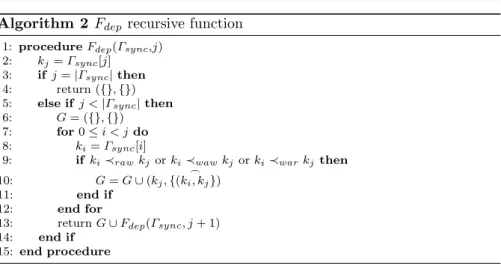
Definition 18 From the synchronized ordered list of computation kernels Γsync, the dependency graph of the computations Γdep(V, A) is obtained from the call Fdep(Γsync, 0), where Fdep is the recursive function defined in Algorithm 2.
This constructive function is possible because the input is an ordered list. Actually, if ki ≺ kj then i < j. As a result, ki is already in V when the arc (
_
ki, kj) is built.
One can note that Γdep only takes into account a single time iteration. A complete dependency graph of the simulation could be built. This is a possible extension of this work.
Proposition 19 The directed graph Γdep is an acyclic graph.
As a result of the hybrid parallelization, each resource 0 ≤ r ≤ p − 1 perform a multi-stencil program, defined by
MSPr(Mr, Φr, Dr, N , ∆r, T, Γdep).
The set of computations Γdep is a dependency graph between computation kernels ki of Γ and synchronizations of kernels added into Γsync. Γdep can be built from the call to
Algorithm 2 Fdep recursive function 1: procedure Fdep(Γsync,j)
2: kj= Γsync[j]
3: if j = |Γsync| then
4: return ({}, {}) 5: else if j < |Γsync| then
6: G = ({}, {}) 7: for 0 ≤ i < j do 8: ki= Γsync[i]
9: if ki≺rawkjor ki≺wawkjor ki≺warkjthen
10: G = G ∪ (kj, {( _
ki, kj})
11: end if
12: end for
13: return G ∪ Fdep(Γsync, j + 1)
14: end if 15: end procedure
Example Figure 7 gives an example of MSP program. From Γsyncthat has been built in Equation (3), the dependency DAG can be built. For example, as k4computes F and k6reads F , k4and k6becomes vertices of Γdep, and an arc (
_
k4, k6) is added to Γdep. The overall Γdepbuilt from the call to Fdep(Γsync, 0) is drawn in Figure 8. By building synchronizations as defined in Definitions (6), (7) and (8), dependencies are respected. For example, ksync0;1 read and write B which guarantees that k0;1syncis performed after k0 and before k1.
k0 k0;1sync k1 k2 k1;4sync k3 k4 k5 k6 k7 k7;8sync k8
Fig. 8: Γdep of the example of program of Figure 7
5.3 Static scheduling
In this section we detail a static scheduling of Γdep by using minimal series-parallel directed acyclic graphs. Such a static scheduling may not be the most efficient one, but it offers a simple fork/join task model which makes possible the design of a performance model. Moreover, such a scheduling offers a simple way to propose a fusion optimization.
In 1982, Valdes & Al [31] have defined the class of Minimal Series-Parallel DAGs (MSPD). Such a graph can be decomposed as a serie-parallel tree,
k0 k1
k2 k3
Fig. 9: Over-constraint on the forbid-den N shape. S P k0 k2 P k1 k3
Fig. 10: TSP tree of Fig. 9.
denoted T SP , where each leaf is a vertex of the MSPD it represents, and whose internal nodes are labeled S or P to indicate whether the two sub-trees form a sequence or parallel composition. Such a tree can be considered as a fork-join model and as a static scheduling. An example is given in Fig. 10.
Valdes & Al [31] have identified a forbidden shape, or sub-graph, called N , such that a DAG without this shape is MSPD.
Thus, as Γdep is a DAG, by removing N-Shapes it is transformed to a MSPD. The intuition is illustrated in Fig. 9. Considering the figure with-out the dashed line, the sub graph forms a ”N” shape. The fact is that this shape cannot be represented as a composition of sequences or parallel executions. To remove such forbidden N-shapes of Γdep = (V, E), we have chosen to apply an over-constraint with the relation k0 ≺ k3, such that a complete bipartite graph is created for the sub-dag as illustrated in Fig-ure 9. By adding this arc to the DAG, it is possible to identify its execution as sequence(parallel(k0; k2); parallel(k1; k3)) represented by the TSP tree of Fig. 10.
After these over-constraints are applied, Γdep is MSPD. Valdes & Al [31] have proposed a linear algorithm to know if a DAG is MSPD and, if it is, to decompose it to its associated binary decomposition tree. As a result, the binary tree decomposition algorithm of Valdes & Al can be applied on Γdepto get the T SP static scheduling of the multi-stencil program.
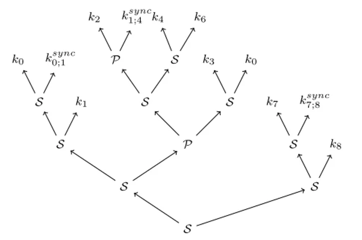
Example From Γdepillustrated in Fig. 8 the TSP tree represented in Fig. 11 can be computed.
5.4 Fusion optimization
Using MSL, it is possible to ask for data parallelization of the application, or for an hybrid parallelization. Even though the MSL language is not dedi-cated to produce very optimized independent stencil codes, but to produce the parallel orchestration of computations, building the T SP tree makes available an easy optimization when the data parallelization technique is the only one used. This optimization consists in proposing a valid merge of some compu-tation kernels inside a single space loop. This is called a fusion. As previously
S S S S k0 ksync0;1 k1 S S k7 k sync 7;8 k8 P S k3 k0 S P k2 k sync 1;4 S k4 k6
Fig. 11: Serie-Parallel tree decomposition of the example of program of Figure 7
explained in Section 3, MSL restrict the definition of a numerical computation by writing a single quantity at a time which avoids errors in manual fusion or counter-productive fusions for task parallelization. MSF guarantees that pro-posed fusions are correct and will not cause errors in the final results of the simulation.
Those fusions can be computed from the canonical form of the T SP tree decomposition. The canonical form consists in recursively merging successive S vertices or successive P vertices of T SP .
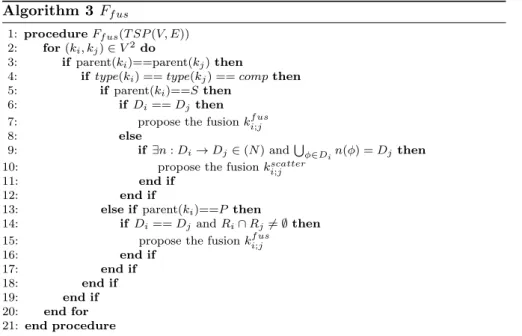
The fusion function Ff usis described in Algorithm 3, where the parent(k) function returns the parent vertex of k in the tree, and where kf usi;j represents the fusion of kiand kjkeeping the sequential order i; j if i is computed before j in T SP . Finally, type(k) returns comp if the kernel is a computation kernel, and sync or red otherwise.
We are not arguing that such a simple fusion algorithm could be as good as complex cache optimization techniques which can be found in stencil DSLs [30] for example. However, this fusion takes place at a different level and can bring performance improvements as illustrated in Section 6. This fusion algorithm relies on the following observations.
First, two successive computation kernels ki and kj which are under the same parent vertex S in TSP are, by construction, data dependent. As a result, what is written by the first one is read by the second one. Thus, wi the quantity written by ki is common to these computations. Thus, if the computation domains verify Di = Dj, the fusion of ki and kj will decrease cache misses.
Second, two successive computation kernels ki and kj which are under the same parent vertex P in TSP are not, by construction, data dependent. However, if the computation domains verify Di = Dj, and if Ri∩ Rj 6= ∅
Algorithm 3 Ff us
1: procedure Ff us(T SP (V, E))
2: for (ki, kj) ∈ V2do
3: if parent(ki)==parent(kj) then
4: if type(ki) == type(kj) == comp then
5: if parent(ki)==S then
6: if Di== Dj then
7: propose the fusion kf usi;j
8: else
9: if ∃n : Di→ Dj∈ (N ) andSφ∈Din(φ) = Djthen
10: propose the fusion kscatter
i;j
11: end if
12: end if
13: else if parent(ki)==P then
14: if Di== Dj and Ri∩ Rj6= ∅ then
15: propose the fusion kf usi;j
16: end if 17: end if 18: end if 19: end if 20: end for 21: end procedure
cache misses could also be decreased by the fusion kf usi;j . These two cases are illustrated by Fig. 12 and Fig. 13.
P ki [Di] kj [Dj] P kf usi;j [Di] Di= Dj
Fig. 12: First fusion case.
S ki [Di] kj [Dj] S kf usi;j [Di] Di= Dj Ri∩ Rj6= ∅
Fig. 13: Second fusion case.
Third, an additional fusion case is possible and more tricky to find. Sim-ilarly to the first observation, two successive computation kernels ki and kj which are under the same parent vertex S in TSP are data dependent and
what is written by the first one is read by the second one. The construction of the tree also guarantees that synchronizations are not needed between these computations, otherwise a ksyncwould have been inserted between them (in-herited from Γsync). Thus, wi the quantity written by ki is common to these computations. Considering the following:
– Di6= Dj, which means that loop fusion is by default not possible,
– (rj, nj) is the pair read by kjfor which rj = wiand for which nj : Dj → Dim the fusion of ki and kj is possible if and only if ∃n : Di→ Dj ∈ N such that
[
φ∈Di
n(φ) = Dj
This means that even if domains are different, a loop fusion is possible if an adequate neighborhood function can be found. One can note that this particular fusion case is equivalent to a scatter optimization, often used when using unstructured meshes. One can also note that the computation kj will be written in a different manner if a scatter fusion is performed or not. This particular case is illustrated in Fig. 14.
S ki [Di] kj [Dj] S kscatter i;j [Di] Di6= Dj ∃n : Di→ Dj S φ∈Din(φ) = Dj
Fig. 14: Third fusion case.
The developer will be notified of fusions in the output of MSC. This is not a problem by using MSF as the fusion is proposed before the developer actually write the numerical code of kj.
5.5 Overall compilation process
MSC takes a MSL file written using the grammar described in Section 4, as well as the Generic Assembly presented in Fig. 5 as inputs, and generates a specialized component assembly that manages the parallel orchestration of the computations of the simulation. In this final assembly, that could be compared to a pattern or a skeleton of the simulation, the developer still has to fill-in the functions corresponding to the various computation kernels by using the DDS instantiation chosen into the specialized assembly. The overall behavior of the compiler is as follows:
1. it parses the MSL input file and generates Γ , the list of computation ker-nels,
2. from Γ , it builds Γsync, the list including synchronizations for data paral-lelism using Algorithm Fsync introduced in Section 5,
3. from Γsync, it builds Γdep, the DAG supporting hybrid parallelism using Algorithm Fdep introduced in Section 5,
4. it then removes the N-Shapes from Γdepto get a MSPD graph, and gener-ates its serie-parallel binary tree decomposition T SP ,
5. it performs the fusion of kernels in T SP if required (data parallelization only),
6. it transforms GA to generate its output specialized component assembly. The last step of this compilation process is detailed below. It is composed of four steps:
1. it instantiates DDS and Data components by using components imple-mented by a third party HPC specialist,
2. it generates the structure of K components responsible for each computa-tion kernel of the simulacomputa-tion,
3. it generates a new Scheduler component,
4. it replaces the Computations component of GA by a generated sub-assembly that matches T SP by using Scheduler, K and Sync components.
New components have been introduced above and need to be explained. A K component is a component into which the developer will write numerical code. It could represents a single computation kernel described by the nu-merician using MSL, or it could represents the fusion of multiple computation kernels. In any case the name of the generated component will use kernel iden-tifiers used in the MSL description. A K kernel is composed of m use ports that are used to be connected to the m quantities needed by the computa-tion (i.e., the numerical code). The component also exposes a provide port to be connected to the Scheduler component. Interfaces of a K component are represented in Fig. 15a.
A Sync component is a static component (not generated) composed of a use-multiple port which is used to request synchronizations for all quantities it is linked to (Data). The component also exposes a provide port to be connected to the Scheduler component. The Sync component is represented in Fig. 15b. Finally, the Scheduler component is the component responsible for imple-menting the T SP tree computed by MSC. Thus, this component represents the specific parallel orchestration of computations. It exposes as many use ports as there are instances of K components to call (i.e., computations and fusions of computations). The component also exposes a provide port to be connected to the T ime component. Interfaces of a Scheduler component are represented in Fig. 15c.
To illustrate how a specialized assembly is generated, the specialized as-sembly of the example that has been used throughout this paper is represented in Fig. 16.
K ∗ (a) K Sync m (b) Sync Scheduler ∗ (c) Scheduler Fig. 15: Specific components used to transform GA to the specialized compo-nent assembly of the simulation.
Driver start m T ime Scheduler A B ... 1 2 3 cart k0 1 2 Sync(0, 1) 3 ...
Fig. 16: Sub-part of the specialized assembly generated by MSC from the ex-ample of the exex-ample of Fig.7 used throughout the paper. For readability some connections are represented by numbers instead of lines. The entire assembly is generated by MSC, however some components are automatically generated by MSC (in green), some are written by HPC specialists (in red) and others by the developer (in blue).
5.6 Performance model
In this subsection we introduce two performance models, one for the data parallelization technique, and one for the hybrid data and task parallelization technique, both previously explained.
The performance model for the data parallelization technique is inspired by the Bulk Synchronous Parallel model. We consider that each process handles its own sub-domain that has been distributed in a perfectly balanced way. The performance model describes the computation time as the sum of the sequential time divided by the number of processes, and of the time spent in communications between processes. Thus, for
– TSEQ the sequential reference time, – P the total number of processes, – TCOM the communications time, the total computation time is
T =TSEQ
Thus, when the number of processes P increase in data parallelization, the performance model limit is TCOM
lim
P →+∞T = TCOM. (6)
As a result, the critical point for performance is when TCOM ≥ TSEQP , which happens naturally in data parallelization as TCOM will increase with the number of processes, and TSEQ
P decrease with the number of processes. This limitation is always true, but can be delayed by different strategies. First, it is possible to overlap communications and computations. Second, it is possible to introduce another kind of parallelization, task parallelization. Thus, for the same total number of processes, only a part of them are used for data parallelization, and the rest are used for task parallelism. As a result, TSEQ
P will continue to decrease but TCOM will increase later. This second strategy is the one studied in the following hybrid performance model.
For an hybrid (data and task) parallelization technique, and for – Pdatathe number of processes used for data parallelization,
– Ptask the number of processes used for task parallelization, such that P = Pdata× Ptask is the total number of processes used,
– Ttask the overhead time due to task parallelization technique, – and Ftask the task parallelization degree of the application, the total computation time is
T = TSEQ
Pdata× Ftask
+ TCOM+ Ttask (7)
The time overhead due to task parallelization can be represented as the time spent to create a pool of threads and the time spent to synchronize those threads. Thus, for
– Tcr the total time to create the pool of threads (may happened more than once),
– Tsync the total time spent to synchronize threads, the overhead is
Ttask= Tcr+ Tsync.
The task parallelization degree of the application Ftask is the limitation of a task parallelization technique. As explained before, a task parallelization technique is based on the dependency graph of the application. Thus, this dependency graph must expose enough parallelism for the number of available threads. For this performance model we consider that
Ftask= Ptask,
however, as it will be illustrated in Section 6 Ftask is more difficult to estab-lish. Actually, the lower and upper bounds of Ftask are constrained by the dependency graph of the application.
As a result when Pdata is small a data parallelization technique may be more efficient, while an hybrid parallelization could be interesting at some point to improve performance. The question is: when is it interesting to use hybrid parallelization ? This paper does not propose an intelligent system to answer this question automatically, however, it offers a way to understand how to answer the question. To answer this question let’s consider the two parallelization techniques, data only and hybrid. We denote
– Pdata1the total number of processes entirely used by the data only
paral-lelization,
– Pdata2 the number of processes used for data parallelization in the hybrid
parallelization,
– and Ptaskthe number of processes used for task parallelization in the hybrid parallelization,
– such that Pdata1= Pdata2× Ptask.
We search the point where the data parallelization is less efficient than the hybrid parallelization. Thus,
TSEQ Pdata1 + TCOM 1≥ TSEQ Pdata2× Ptask + TCOM 2+ Ttask.
This happens when
TCOM 1≥ TCOM 2+ Ttask (8)
This performance model will be validated and will help explain results of Section 6.
6 Evaluation
This section first presents the implementation details chosen to evaluate MSF in this paper, and the studied use case. Then, the compilation time of MSC is evaluated before analyzing both available parallelization techniques, data and hybrid (data and task). Finally, the impact of kernels fusions is studied.
6.1 Implementation details
The main choices to take when implementing a specialized assembly of GA concern the technologies used for data and task parallelizations, i.e., imple-mentation choices of DDS and Scheduler components.
For the data-parallelization, as already detailed many times throughout the paper, a third party HPC specialist is responsible for implementing DDS and Data using a chosen library or external language and by following the specified interfaces of these two components. To evaluate MSF, we have played the role of HPC specialists and have implemented these components using SkelGIS, a
C++ embedded DSL [10] that proposes a distributed Cartesian mesh as well as user API to manipulate structures while hiding their underlying distribution. For task parallelism, we have chosen to use OpenMP [13] to generate the code of the Scheduler component. OpenMP targets shared-memory platforms only. Although the version 4 of OpenMP has introduced explicit support for dynamic task scheduling, our implementation only requires version 3 whose fork-join model is well suited for the static scheduling introduced in Section 5. The use of dynamic schedulers, such as provided by libgomp2, StarPU [2], or XKaapi [17], to directly execute the DAG Γdep is left to future work.
As a result, MSC generates a hybrid code which uses both SkelGIS and OpenMP. It also generates the structure of K components where the developer must provide local sequential implementations of the kernels using SkelGIS API.
6.2 Use case description
All evaluations presented in this section are based on a real case study of the shallow-Water Equations as solved in the FullSWOF2D3[10,16] code from the MAPMO laboratory, University of Orl´eans. In 2013, a full SkelGIS implemen-tation of this use case has been performed by numericians and developers of the MAPMO laboratory [9, 10, 12]. From this implementation we have kept the code of computation kernels to directly use it into K components. Com-pared to a full SkelGIS implementation, where synchronizations and fusions are handled manually, MSF automatically compute where synchronizations are needed and how to perform a fusion without errors. To evaluate MSF on this use case we have described the FullSWOF2D simulation by using MSL. FullSWOF2D contains 3 mesh entities, 7 computation domains, 48 data and 98 computations (32 stencil kernels and 66 local kernels). Performances of the obtained implementation are compared to the plain SkelGIS implementation to show that no overheads are introduced by MSF by using L2C.
6.3 Multi-Stencil Compiler evaluation
Table 1 illustrates the execution time of each step of MSC for the FullSWOF2D example. This has been computed on a laptop with a dual-core Intel Core i5 1.4 GHz, and 8 GB of DDR3. MSC has been implemented in Python 2. While the overall time of 4.6 seconds remains reasonable for a real case study, one can notice that the computation of the T SP tree is by far the longest step. As a matter of fact, the complexity of the algorithm for N-shapes removal is O(n3). If this complexity is not a problem at the moment and onto this use case it could become one for just-in-time compilation or more complex simulations. The replacement of the static scheduling by a dynamic scheduling
2
https://gcc.gnu.org/projects/gomp/
using dedicated tools (such as OpenMP 4, StarPU etc.) should solve this in the future.
Step Parser Γsync Γdep T SP
Time (ms) 1 2 4.2 3998.5
% 0.022 0.043 0.09 86.6
Table 1: Execution times of the MSL compiler
6.4 Data parallelism evaluation
In this part, we disable task-parallelism to focus on data-parallelism. Two versions of the code are compared in this section: first a plain SkelGIS im-plementation of FullSWOF2D, where synchronizations and fusions are han-dled manually; second, a MSF over SkelGIS version where synchronizations and fusions are automatically handled. SkelGIS has already been evaluated in comparison with a native MPI implementation for the FullSWOF2D exam-ple [10]. For this reason, this section uses the plain SkelGIS imexam-plementation as the reference version. This enables to evaluate both the choices made by MSC as well as the potential overheads of using L2C [5] that is not used in the plain SkelGIS version. The evaluations have been performed on the Curie su-percomputer (TGCC, France) described in Table 2. Each evaluation has been performed nine times and the median is presented in results.
TGCC Curie Thin Nodes Processor 2×SandyBridge (2.7 GHz) Cores/node 16 RAM/node 64 GB RAM/core 4GB #Nodes 5040 Compiler [-O3] gcc 4.9.1 MPI Bullxmpi
Table 2: Hardware configuration of TGCC Curie Thin nodes.
Weak scaling Figures 17, 18 and 19 respectively show weak scaling exper-iments tha twe have conducted. Four computation domains are evaluated: 400 × 400 cells by core, 600 × 600 cells by core and 800 × 800 cells by core, from 16 to 16,384 cores, as summarized in Table 3.
From these results, one can notice, first, that performances of MSF are very close to the reference version using plain SkelGIS. This is a very good
Domain size per core Number of iterations
400 × 400 200
600 × 600 200
800 × 800 200
Table 3: Weak scaling experiments of Fig. 17, Fig. 18 and Fig. 19.
24 25 26 27 28 29 210 211 212 213 214 cores 0 5 10 15 20 25 30 time (s) MSF over SkelGIS SkelGIS
Fig. 17: weak-scaling with 400 × 400 domain per core and 200 time itera-tions. 24 25 26 27 28 29 210 211 212 213 214 cores 0 10 20 30 40 50 60 70 time (s) MSF over SkelGIS SkelGIS
Fig. 18: weak-scaling with 600 × 600 domain per core and 200 time itera-tions. 24 25 26 27 28 29 210 211 212 213 214 cores 0 20 40 60 80 100 time (s) MSF over SkelGIS SkelGIS
Fig. 19: weak-scaling with 800 × 800 domain per core and 200 time iterations.
result which shows first that MSC performs good synchronizations and fusions, and second that overheads introduced by L2C are limited thanks to a good component granularity in the Generic Assembly.
However, it seems that a slightly drop of performance happens when the do-main size per core increases. This performance decrease is really small though, with a maximum difference between the two versions of 2.83% in Fig. 19.
25 26 27 28 29 210 211 212 213 214 cores 2-2 2-1 20 21 22 23 24 25 26 27 28
iterations per second
Ideal
MSL + SkelGIS SkelGIS
Fig. 20: Strong scaling on a 10k × 10k domain and 1000 time iterations.
The only noticeable difference between the two versions are due to L2C which load dynamic libraries at runtime. Because of this particularity, compo-nents of L2C are compiled with the -fpic compilation flag4 while the SkelGIS version does not. This flag can have slight positive or negative effects on code performance depending on the situation and might be responsible for the ob-served difference.
Strong scaling Figure 20 shows the number of iteration per second for a 10k×10k global domain size from 16 to 16,384 cores. The total number of time iterations for this benchmark is 1000. In addition to the reference SkelGIS version, the ideal strong scaling is also plotted in the figure.
First, one can notice that the strong scaling evaluated for the MSF version is close to the ideal speedup up to 16,384 cores, which is a very good result. Moreover, no overheads are introduced by MSF which shows that automatic synchronizations and automatic fusions enable the same level of performance than the one manually written into the plain SkelGIS version. Finally, no overheads are introduced by components of L2C. A small behavior difference can be noticed with 29= 512 cores, however this variation is no longer observed with 1024 cores.
6.5 Hybrid parallelism evaluation
In this section, we add task parallelism to evaluate the hybrid parallelization offered by MSF. The MSF implementation evaluated in this paper relies on SkelGIS and OpenMP.
The series-parallel tree decomposition T SP of this simulation, extracted by MSC, is composed of 17 nodes labeled as sequence S and 18 nodes labeled as parallel P.
We define the level of parallelism as the number of parallel tasks inside one fork of the fork/join model. The fork/join model obtained for FullSWOF2D is composed of 18 fork phases (corresponding to P nodes of T SP ). Table 4 represents the number of time (denoted frequency) a given level of parallelism is obtained inside fork phases.
Level 1 2 3 4 6 10 12 16
Frequency 2 1 3 5 3 1 1 2
Table 4: Parallelism level and the number of times this parallelism level appears into fork phases.
One can notice that the level of task parallelism extracted from the Shallow water equations is limited by two sequential parts in the application (level 1). Moreover, a level of 16 parallel tasks is reached two times, and five times for the fourth level. This means that if two cores are dedicated to task parallelism, the two sequential parts of the code will not take advantage of these two cores, and that no part of the code would benefit from more than 16 cores. The task parallelism, as proposed in this paper (i.e., where each kernel is a task) is therefore insufficient to take advantage of a single node of modern clusters that typically supports more than 16 cores.
1 2 4 8 16 32 64 128 256 512 1024 2048 cores 10-4 10-3 10-2 10-1 time (s) Computations Communications
Fig. 21: Computation vs communication times for a single time iteration using the data parallelization technique.