HAL Id: hal-02419516
https://hal.archives-ouvertes.fr/hal-02419516
Submitted on 12 Jan 2021
HAL is a multi-disciplinary open access
archive for the deposit and dissemination of
sci-entific research documents, whether they are
pub-lished or not. The documents may come from
teaching and research institutions in France or
L’archive ouverte pluridisciplinaire HAL, est
destinée au dépôt et à la diffusion de documents
scientifiques de niveau recherche, publiés ou non,
émanant des établissements d’enseignement et de
recherche français ou étrangers, des laboratoires
Numerical study on laminar flame velocity of
hydrogen-air combustion under water spray effects
Guodong Gai, Sergey Kudriakov, Bernd Rogg, Abdellah Hadjadj, Etienne
Studer, Olivier Thomine
To cite this version:
Guodong Gai, Sergey Kudriakov, Bernd Rogg, Abdellah Hadjadj, Etienne Studer, et al.. Numerical
study on laminar flame velocity of hydrogen-air combustion under water spray effects. International
Journal of Hydrogen Energy, Elsevier, 2019, 44 (31), pp.17015-17029. �10.1016/j.ijhydene.2019.04.225�.
�hal-02419516�
Numerical study on laminar flame velocity of hydrogen-air combustion under
water spray e
ffects
Guodong Gaia,∗, Sergey Kudriakova, Bernd Roggb, Abdellah Hadjadjc, Etienne Studera, Olivier Thominea
aDEN-DM2S-STMF, CEA, Universit´e Paris-Saclay, France bFaculty of Mechanical Engineering, Ruhr-University, 44780 Bochum, Germany
cNormandie University, INSA of Rouen, CNRS, CORIA, 76000 Rouen, France
Abstract
In the context of hydrogen safety and explosions in hydrogen-oxygen systems, numerical simulations of laminar, premixed, hydrogen/air flames propagating freely into a spray of liquid water are carried out. The effects on the flame velocity of hydrogen/air flames of droplet size, liquid-water volume fraction, and mixture composition are numerically investigated. In particular, an effective reduction of the flame velocity is shown to occur through the influence of water spray.
To complement and extend the numerical results and the only scarcely available experimental results, a “Laminar Flame Velocity under Droplet Evaporation Model” (LVDEM) based on an energy balance of the overall spray-flame system is developed and proposed. It is shown that the estimation of laminar flame velocities obtained using the LVDEM model generally agrees well with the experimental and numerical data.
Keywords:
Combustion, Laminar Flame Velocity, Water Spray, Hydrogen Safety
1. Introduction
Spray systems are used as emergency devices for the mitigation of effects of explosions involving deflagration waves. Such systems are installed, for example, inside industrial buildings or on offshore facilities. Spray noz-zles are also present inside some nuclear reactor build-ings, and they are designed for preserving the contain-ment integrity in case of a severe accident [1,2]. In case of an explosion, for a spray system to act successfully upon unwanted premixed-flame propagation, an under-standing of, (i), the dynamics of the water spray exposed to the explosion-induced flow field, and, (ii), the ability of the spray to mitigate the explosion, is needed.
The droplets generated by industrial water-spray sys-tems have a Sauter mean diameter of the order of 100 µm. For example, the spray systems usually installed on o ff-shore platforms generate droplets of Sauter mean diame-ters in the range 200-700 µm [3] while those installed in-side reactor buildings produce droplets of a Sauter mean diameter in the range 280-340 µm [1]. Numerous inves-tigations have demonstrated [4–6] that, if certain con-ditions are met, large droplets might break up and cas-cade down into a large number of small droplets, i.e.,
∗
Corresponding author
Email address: guodong.gai@cea.fr (Guodong Gai)
droplets of a volume mean diameter of approximately 10 µm. These small droplets have the capability to evap-orate fully, or almost fully, inside a laminar flame thus modifying the flame structure. Experimental results de-voted to the interaction of a laminar flame with small wa-ter droplets are scarce. Laboratory-scale tests reported in [7] showed that water droplets with diameters of the order of 10 µm have a similar influence on the struc-ture of inert methane-air mixstruc-tures as water vapor. Early small scale experiments [8] as well as recent small and medium scale experiments using hydrogen [9], [10] have revealed that sprays containing small-size droplets can be effective against premixed combustion. The experi-ments performed in [11] were devoted to hydrogen-air laminar flame velocity measurements in the presence of water mist.
In the context of spray-decelerated or spray-retarded deflagration waves that have originated from explosions, laminar-flame velocity – occasionally also termed “lam-inar flame speed” – is an important physical quantity. In particular, most of the combustion models used for sim-ulation of large-scale, turbulent premixed combustion – see, e.g., [12–16] – contain the laminar-flame velocity as input parameter which has to be procured by some means such as suitable numerical simulation or suitable experi-ments. In the literature several correlations exist [17,18]
Nomenclature
A0 area of the burner mouth, m2
Af area of the flame front, m2
cp,g gas heat capacity at constant pressure, J/K/kg
D diameter of the droplet, µm Dc,1 first critical droplet diameter, µm
Dc,2 second critical droplet diameter, µm
Ea global activation energy, kcal/mol
l latent heat of evaporation, kJ/kg ˙
m evaporation rate of droplets, kg/s nvol number of droplets per volume, m−3
P0 initial pressure, bar
r0 initial radius of the droplet, µm
R universal gas constant, J/K/mol SL laminar flame velocity, m/s
tc chemical reaction time, s
tq quenching time, s
T0 initial temperature, K
v0 average flow velocity in the burner, m/s
Vb burnt gas velocity, m/s
Vf fresh gas velocity, m/s
XH2 molar fraction of hydrogen, dimensionless
y coordinates in the Cosilab code, mm YH2 mass fraction of hydrogen, dimensionless
α liquid volumetric fraction, dimensionless αg thermal diffusivity, m2/s
δ flame thickness, m
η hydrogen-air mole ratio, dimensionless λ thermal conductivity, W/m/K
µg dynamic viscosity of gas, Pa · s
ρ mass density, kg/m3
φ equivalence ratio, dimensionless
Nu Nusselt number, dimensionless S c Schmidt number, dimensionless Pe Peclet number, dimensionless Pr Prandt number, dimensionless Re Reynolds number, dimensionless S h Sherwood number, dimensionless Le Lewis number, dimensionless
BM Spalding mass transfer number,
dimen-sionless
BT Spalding temperature transfer number,
di-mensionless
F Correction factor in evaporation model, dimensionless
AIBC Adiabatic IsoBaric complete Combustion
AICC Adiabatic IsoChoric complete Combustion
characterizing the flame speed of purely gaseous laminar
hydrogen/air flames as a function of the mixture equiva-lence ratio. However, the small water droplets of a water spray modify the internal structure of the laminar flame and hence reduce its velocity. Thus a model is needed which takes into account the effect of water spray on flame structure and burning velocity.
In this paper, a “Laminar Flame Velocity under Droplet Evaporation Model” – abbreviated LVDEM – for hydrogen/air mixtures is proposed. This model has been constructed using the idea of Ballal and Lefebvre [19] who considered the energy balance inside the flame zone. The most crucial step is the model validation. For this purpose, the results obtained with the dedicated code Cosilab [20] and the experimental results of [11] are used. The results obtained using the LVDEM model generally agree well with the experimental and numeri-cal data.
2. Phenomenology of Computed Flame Structures In this section, a description of the main phenomena related to the interaction of laminar hydrogen/air pre-mixed, freely propagating flames with small droplets of a liquid water spray is given. The “small droplets” means droplets typically having a volume mean diameter of the order of 10 µm or smaller. For the numerical simulations, the Cosilab code [20] has been our main tool. This code can compute the internal structure of a laminar steady flame, with or without the presence of a liquid-water spray[21–23]. For completeness, the algorithm used in the code is shortly summarized in Appendix A. The main idea in using the code is to identify the mechanisms re-sponsible for flame-droplets interactions, which will sub-sequently be used in our LVDEM model construction.
Specifically, two cases of hydrogen-air combustion are considered, i.e., cases without and cases with water spray. The purely gaseous cases, i.e., the cases without water spray serve as a reference for the two-phase cases with water spray.
In the numerical simulations with Cosilab, detailed chemistry, thermodynamics and molecular transport were taken into account. Specifically, the hydrogen/air system considered in the simulations comprised 10 chemical species which participate in 21 homogeneous reactions. For details of the reaction mechanism and the associated data, [24] should be consulted.
The governing equations for a one-dimensional, flat, spray flame propagating at low Mach number can be found, e.g., in [25], Chaps. 1, 5 and 11. In particular, the dependent variables are discussed in [25] as well as the so-called cold and hot boundaries at either end of the computational domain together with the suitable bound-ary conditions to be applied there. In addition, a detailed description of the so-called burning rate-eigenvalue can
be found, in [25], Chap. 5, and how from that quantity in general the gaseous flow velocity throughout the flame is recovered and, especially, how the burning rate or flame speed is derived from it. Numerical solution methods for the problem are discussed, e.g., in [26] and [21]. There-fore, the governing equations and their solutions are not further discussed here.
At the cold flame boundary – which from the subse-quent figures can be seen to be located at the left bound-ary of the computational domain – the gaseous com-position of pure hydrogen and air is given in terms of the fuel-air equivalence ratio, φ, and the temperature, T0, is prescribed. Since the deflagration waves
consid-ered propagate in an open system at low Mach numbers, we adopt the low-Mach-number approximation [25] and take the pressure, P0, as spatially uniform and constant.
For the cases with water spray, the spray is added at the cold boundary and is taken as mono-disperse with given droplet diameter D and given liquid volume-fraction α. At the cold boundary, zero slip-velocity between gas and liquid phase is assumed. Furthermore, liquid-load or vol-ume fraction in this work are such that the case of a so-called thin spray is considered, that is effects of droplet break-up and agglomeration are neglected.
Interaction of the gaseous and the liquid flame princi-pally occurs throughout the computational domain that, theoretically, extends from minus to plus infinity. Nat-urally, the computer-realized extension of the computa-tional domain is finite, and its finite size has been chosen such that the boundary conditions are cleanly satisfied – for details see [25] – so that the flame speed or burn-ing rate calculated is virtually independent of the size of the computational domain. As will be seen from the following figures, at the cold boundary the interaction of spray and gas consists essentially in spray evapora-tion. Some bit downstream, in the preheat zone where chemical reaction is negligible yet computed, the gas be-gins to accelerate due to the heat gained from the reac-tion zone by conducreac-tion against flow direcreac-tion. In the reaction zone primarily the conduction and the reaction phenomena balance each other, while in the downstream recombination zone the dominating phenomena are the convection and the recombination reactions [25].
In this work, droplets are assumed to be totally evap-orated when the ratio of local to initial droplet size has fallen below the computational roundoff-error – in the graphs below, the droplet diameter or radius is then vir-tually zero. For the flame structures to be presented in Figs. 1 to5, the numerical values used for the condi-tions just described are summarized in Table1. The fol-lowing comparison of the purely gaseous reference case, i.e., the case without water spray, and the two-phase case with water spray exposes details of the flame structures and also clearly shows the influence of the droplets on
case φ T0[K] P0[bar] D [µm] α
gaseous 1.6 300 1.013 -
-gas/spray 1.6 300 1.013 6 10−4
Table 1: Parameters used with Cosilab to obtain the results shown in Figs.1to5.
the overall flame structure. At this stage it is important to note that in Figs.1 to5 only a small portion of the actual computational domain is shown, namely that por-tion that is essential to visually capture the flame struc-tures. In the computations the domain was substantially increased towards both the cold and the hot boundary to ensure that the boundary conditions were cleanly satis-fied at either boundary to avoid the prediction of inaccu-rate flame structures and hence burning velocities, e.g., due to artificial heat losses to the cold boundary.
In the Figs. 1 to 5 subsequently presented and dis-cussed, the results for the purely gaseous reference case without water spray are shown as dashed lines whereas the results for the two-phase case with water spray are represented by solid lines.
2.1. Gasphase Temperature
Shown in Fig. 1 are the profiles of temperature and volumetric heat release. A series of computations with differently sized domains of total length of up to 6 mmwas carried out in order to satisfy cleanly both the upstream and downstream boundary conditions. The results shown here were obtained on a non-uniform, self-adaptive computational mesh with a mean cell size of ∆y = 12 µm. The mesh is substantially denser (∆ymin = 1.1841 µm) within the thin reaction zone and
expands towards the cold and the hot boundary (∆ymax=
41.84 µm), respectively.
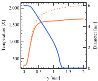
From Fig.1it is seen that the temperature in the reac-tion zone and further downstream is drastically reduced as a consequence of the droplets evaporating in the flame – e.g., at y= 2 mm the temperature is reduced from ap-proximately 2100 K to apap-proximately 1700 K. Accord-ingly, the rate of temperature increase is reduced inside the flame as can be inferred from the difference of the heat-release-rate profiles. The cooling effect due to the presence of droplets is particularly important in both the preheat zone and the reaction zone – this is where evap-oration is strongest as will also seen below when consid-ering the variation of droplet diameter though the flame. At this stage is appropriate to define the “flame thick-ness” δ. Throughout this section, the flame thickness will be taken as the width of the preheat zone (in Fig.1for the spray flame ranging approximately from 0.1 mm to 0.4 mm, thus δ ≈ 0.3 mm). Formally this definition of flame thickness can be expressed as the width of that
0 0.5 1 1.5 2 500 1,000 1,500 2,000 2,500 y [mm] T emperature [K ] −2 −1.5 −1 −0.5 0 Heat release rate [x(10 10 J/ s/ m 3 ]
Figure 1: Profiles of temperature ( ) and heat release rate ( ). Dashed lines: reference case without spray for temperature ( ) and heat release rate ( ). Parameters are given in Table1.
spatial zone cut out by the intersection of the tangent to the temperature profile at that location in the flame where the temperature gradient is steepest with, (i), the spatially constant profile at cold boundary temperature, (ii), the straight line with constant slope approximating the slightly rising temperature profile in the post-flame region. It is noted that this definition of flame thickness is popular but, of course, not unique.
In summary, one notes that in the presence of liquid water droplets the cooling effect through convective heat losses of the gasphase to the droplets and through evapo-ration reduce the maximal rate of heat release, thus lead-ing to a lower gas temperature and hence burnlead-ing veloc-ity.
2.2. Species Concentrations
Shown in Fig. 2are profiles of selected species mole fractions through the flame. The variation of the mole fraction of molecular nitrogen, N2, indicates that the
to-tal number of gas moles decreases during combustion ac-companied by spray evaporation. Also, in the two-phase case, the increase of water steam through the flame is not only due to homogeneous chemical reaction but also to evaporation of liquid drops. The mole fraction of the hy-drogen radical, H, increases, reaches its maximum at y= 0.4 mm, and then decreases further downstream.
It can be noted that the evaporation rate increases when the reaction rates and hence gasphase temperature reach high levels. Beyond that, further downstream, the increase of the mole fraction of gaseous water, or water steam, is relatively slow.
0.0 0.2 0.4 0.6 0.8 1.0 1.2 1.4 0.0 0.1 0.2 0.3 0.4 0.5 0.6 y [mm] Mole fraction X [− ]
Figure 2: Profiles of the mole fractions of H2( ) O2( ), H2O
( ), H ( ), and N2( ). Dashed lines: reference case
with-out spray for H2( ), O2( ), H2O ( ), H ( ) and N2
( ). Parameters are given in Table1.
0 0.5 1 1.5 2 500 1,000 1,500 2,000 y [mm] T emperature [K ] 0 2 4 6 Diameter [µ m ]
Figure 3: Spatial variation of droplet diameter ( ) and gasphase temperature ( ). Dashed lines: reference case without spray for the temperature ( ). Parameters are given in Table1.
2.3. Droplet Diameter
Figure 3 shows the variation of the droplet diame-ter through the flame together with the gasphase tem-perature profile. From the figure it can seen that the droplets are not evaporating completely inside the pre-heat zone. Downstream of the prepre-heat zone evapora-tion of the droplets continues, i.e., in the reacevapora-tion zone and even in the post-flame region evaporation of droplets still has a certain influence on the flame propagation and hence burning velocity. Thus, when constructing the LVDEM model below, it will be necessary to estimate the amount of water evaporating inside the preheat zone
(whose thickness corresponds to the flame thickness), which has a direct effect on the flame velocity.
One notices that the droplets rapid evaporation in the zone 0.2 mm < y < 0.5 mm is accompanied by consid-erable temperature reduction, compared to the reference case without spray. The droplet diameter decreases to approximately 3 µm at y =0.8 mm, but are considered totally evaporated only at y=1.3 mm.
2.4. Gasphase Mass Density and Mass Flux
0 0.5 1 1.5 2 0.1 0.2 0.3 0.4 0.5 0.6 0.7 y [mm] Density [k g /m 3 ] 1.8 1.9 2.0 2.1 2.2 Mass flux [k g /s /m 2]
Figure 4: Spatial variation of gas density ( ) and gas mass flux ( ). Dashed lines: reference case without spray for the gas density ( ) and mass flux ( ). Parameters are given in Table1.
Shown in Fig. 4 are the mass density and mass flux variation of the gas mixture during the combustion. For both the purely gaseous reference case and the two-phase case with water spray the gas gasphase mass density pro-files are as expected on physical grounds: they simply express the gas expansion due to the heat released in the homogeneous chemical reactions. The gas mass flux profile of the reference case is uniformly constant as en-forced by overall mass conservation. On the other hand, the gasphase mass-flux profile of the two-phase case in-creases in flow direction due the continuously gained wa-ter steam stemming from liquid-drop evaporation. It can be noted that, of course, the overall mass of liquid and gas is conserved throughout the flame. The mass flux in the two-phase case is lower than the pure gas combustion case, since the laminar flame velocity is reduced by the evaporation of the droplets.
2.5. Gasphase and Droplet Velocity
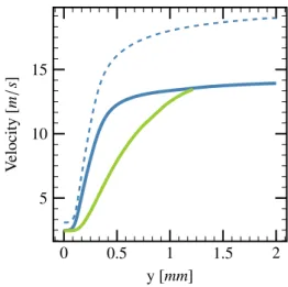
Finally, Fig. 5 shows the profiles of the velocities of gas and liquid through the flame. For the purely gaseous reference case the velocity profile is as expected, namely proportional to the reciprocal of mass density and
0 0.5 1 1.5 2 5 10 15 y [mm] V elocity [m /s ]
Figure 5: Spatial variation of gasphase velocity ( ) and liquid-phase velocity ( ). Dashed lines: reference case without spray for the gas velocity ( ). Parameters are given in Table1.
roughly proportional to temperature. Also the two ve-locity profiles of the two-phase case show the expected behavior. In accordance with the model of a freely prop-agating one-dimensional flame, there is no slip between the phases at the cold boundary. Downstream of the cold boundary, the gasphase velocity then quickly in-creases due to the expansion of the gas. The droplets are dragged by the accelerating gas and hence are also accelerated, but due to their inertia they lag behind the gaseous fluid. This leads to the observed slip between the phases. Further downstream, when the droplets have become very small or have even vanished – see Fig. 3 –, the slip decreases, and at approximately y = 1.2 mm the liquid velocity catches up with the gasphase veloc-ity. The droplets become easier to accelerate due to the evaporation. After y = 1.25 mm, the droplets are to-tally evaporated. In the spray case, overall the gasphase velocity remains substantially lower than in the purely gaseous reference case because of the energy losses due to the droplets evaporation and the addition of steam.
The comparison of the two cases shows that the spray droplets effectively damp, or mitigate, the flame veloc-ity. Specifically, in the cases of Fig. 5, the velocity of the burnt gas is reduced from approximately 18 m/s to approximately 14 m/s.
2.6. Burning Velocity
Flame structures and hence laminar burning velocities for both the purely gaseous reference case and the two-phase case with water spray were computed for a wide range of conditions. The respective results will be pre-sented and discussed below in the context of the LVDEM model.
2.7. Conclusions from the Numerical Results
First, from the numerical results presented so far, it can be concluded that droplets of small diameter greatly af-fect the internal flame structure in terms of temperature, species distribution and gas velocity profiles. Second, the following observation has been made relating to the importance of the amount of water evaporating inside the flame zone: in the present case (D= 6 µm), the droplets do not evaporate completely inside the flame preheat zone which has a thickness of the order of the flame thickness; hence it would be a mistake to assume in a model complete droplet evaporation in that zone. Rather, evaporation takes place in a zone somewhat longer than the preheat zone, i.e., it extends over a region that is wider than the flame thickness.
3. LVDEM model for SLunder droplets evaporation
In this section, the LVDEM numerical model of lam-inar flame velocity based on the energy balance is de-scribed. The comparison between the LVDEM model and the results of the Cosilab code is presented. Experi-mental results are used to validate the two methods. 3.1. Laminar Flame Velocity under Droplet Evaporation
Model
The aim is to construct a model in which several phe-nomena can affect the laminar flame propagation: 1) the evaporation of the droplets will absorb energy released from the chemical reaction; 2) the steam evaporated from the droplets will mix with the remaining gas and change its thermal properties. Ballal [19] has proposed a method to estimate the laminar flame velocity for the evaporation and combustion of fuel droplets using the energy balance inside the flame. The similar idea can be used for the es-timation of the laminar flame velocity in this study. The main assumption of the model is that the quench time of the reaction zone is equal to the chemical reaction time, i.e.
tq= tc, (1)
The quench time can be obtained as the ratio of the excess enthalpy of the reaction zone to the rate of heat loss by conduction to the fresh mixture.
tq =
cp,gρg∆TadδA − l ˙mtcnvolδA
λg(∆Tred/δ)A
, (2)
where the∆Tad = TAIBC−T0,∆Tredis the temperature
re-duction due to the evaporation of droplets; δ is the thick-ness of the flame and A is the area of a considered sur-face; tcis chemical reaction time, nvolis the number
den-sity of the droplets in the mixture; l is the latent heat of the evaporation; cp,gis the gas heat capacity under con-stant pressure, λgis the gas heat conductivity.
Hence tq=
(cp,gρg∆Tad− l ˙mtcnvol)δ2
λg∆Tred
. (3)
Here the flame thickness can be estimated with the laminar flame velocity without spray effects SL,0:
δL=
αg
SL,0, (4)
with αg being the thermal diffusivity of burnt gas
mix-ture, the chemical reaction time of a premixed mixture is given by: tc= δL SL,0 = αg S2L,0, (5) The simulation results of the Cosilab code [20] can be used for the estimation of SL,0. The correlation given by
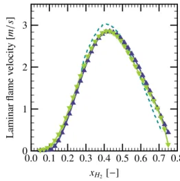
Konnov [18] has also been consulted for the variation of SL,0[m/s] as a function of XH2[vol.%]: SL,0= −1.55236 × 10−9X6H 2+ 3.49519 × 10 −7X5 H2 −2.82975 × 10⁻⁵XH4 2 +9.35480 × 10−4X3 H2− 9.97510 × 10 −3X2 H2 +5.00120 × 10⁻²X H2− 8.32830 × 10 −2. (6) The comparison between these two models is given in Fig.6, where the correlation of Dahoe [17] is also given for comparison. 0.0 0.1 0.2 0.3 0.4 0.5 0.6 0.7 0.8 0 1 2 3 xH2[−] Laminar flame v elocity [m /s ]
Figure 6: Laminar flame velocity evolution for different hydrogen com-position, comparison between three models: Dahoe ( ), the Cosi-lab code ( ) and Konnov ( ).
Since mixtures diluted by steam have lower burnt gas temperatures than undiluted ones, Koroll has proposed a correlation that takes into account the change of thermal diffusivity due to dilution [27]:
SL,w= SL,0· r α dil αpure 1 − Xdil Xdil, f lame ! , (7)
where αdil is the thermal diffusivity of the diluted
mix-ture, αpureis the thermal diffusivity of undiluted mixture,
Xdilstands for the molar fraction of the water steam, and
Xdil, f lame is the maximal molar fraction of steam under which the flame can propagate. This limit water loads can be approximated by the correlation:
Xdil, f lame(η)= 0.507 − 0.2443 · ln(η) − 0.185 · [ln(η)]2 for 0.1 ≤ η ≤ 3,
(8) where η= XH2/Xairis the hydrogen-air mole ratio. The
validation of this correlation can be referred to [27]. The effect of presence of water steam on the hydrogen air combustion has also been discussed in a more recent work of [28], which presents another correlation for SL,w.
Substituting the equation (3) and (5) into the equation (1) gives: δ = λg∆Tred cp,gρg∆Tad− l ˙mnvol(αg/S2L,0) αg S2 L,0 0.5 , (9)
and by applying equation (4), one can have:
SL= αg λg∆Tred cp,gρg∆Tad− l ˙mnvol(αg/S2L,0) αg S2L,0 −0.5 . (10)
The equation (10) is deduced from the energy balance, by taking into consideration of the evaporation process. Combining the equations (7) and (10), the laminar flame velocity can be approximated by:
SL = αg r α dil αpure 1 − Xdil Xdil, f lame ! (11) λg∆Tred cp,gρg∆Tad− l ˙mnvol(αg/S2L,0) αg S2 L,0 −0.5 .
The mass evaporation rate for a droplet ˙mcan be com-puted by using the works of [29,30] as discussed in the above section.
Since the model of [29] gives the mass evaporation rate of one droplet as a function of time at a given temper-ature, one has to estimate the evaporated mass of water droplets during the combustion within the flame thick-ness. As discussed before, the evaporation rate depends on the droplet diameter and the ambient temperature. Thus, its value changes all along the droplet evolution in-side the hot gas mixture. The way to estimate the average mass evaporation rate is presented in the next subsection (point 5).
3.2. Solution Algorithm
Consider now the step-by-step procedure to determine the laminar flame velocity SLunder the influence of
wa-ter droplets. Assume that the initial temperature Tiniand
pressure Piniare known. The free propagating flame
as-sumption is kept in this section.
1. Calculate the initial molar fraction X0,H2, X0,O2,
X0,N2and X0,H2O;
2. Calculate the temperature corresponding to AIBC1 combustion Tadwithout water spray effects;
3. Calculate the laminar flame velocity without water spray effects SL,0using the equation (6) as a
refer-ence flame velocity. This flame velocity can be re-placed by the reference value given by the Cosilab code;
4. Calculate the average physical properties ¯cp,g, ¯λgin
the gas-liquid interaction film, using the “1/3 rule” [29]: ¯ T = Ts+ 1 3(T∞− Ts), (12) ¯ Y = Ys+ 1 3(Y∞− Ys), (13) where the subscript s denotes the surface properties of the droplet and ∞ stands for the properties of the gasphase (for example, the AIBC temperature); 5. Calculate the mean evaporation rate ˙m, as well as
the latent heat l. According to the model of [29], the evaporation rate is calculated by assuming a con-stant ambient temperature. This is not the case in-side the flame thickness. By definition, the gas tem-perature varies from the unburnt gas to the burnt gas. Moreover, the evaporation can affect the tem-perature variation within the flame thickness. Thus, one can calculate the evaporation rate under two AICC2 temperatures, TAICC and 12TAICC, and then
take the average of ˙mTAICCand ˙m12TAICC.
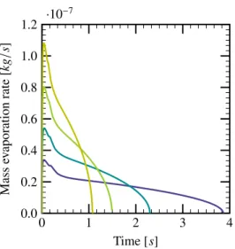
This step is crucial in the algorithm, and these tem-perature values have been chosen by trial and er-ror, in order to minimize the difference between the present results and the experimental results. Fig. 7shows the variation of evaporation rate evolution for different ambient temperatures. Note that the temperatures corresponding to AIBC (1547 K) and AICC (1885 K) combustion are taken into consider-ation, as well as two temperatures (900 K and 1200 K) for comparison. It can be seen that the evapora-tion rate strongly depends on the ambient tempera-ture of the gasphase. One can also estimate that the mean evaporation rate of one single droplet during the combustion process is of the order of magnitude of O(10−8) kg/s for droplet diameter D = 350 µm as presented in Fig. 7. The evaporation rate of the spray is calculated by multiplying the single droplet evaporation rate with the number density of droplets nvol. The effect of the spray evaporation is
consid-ered to be a superposition of all the single droplets.
1Adiabatic IsoBaric complete Combustion 2Adiabatic IsoChoric complete Combustion
0 1 2 3 4 0.0 0.2 0.4 0.6 0.8 1.0 1.2 ·10 −7 Time [s] Mass ev aporation rate [k g /s ]
Figure 7: Influence of ambient temperature on the mass evaporation rate: 900 K ( ), 1200 K ( ), TAIBC= 1547 K ( ) and
TAICC= 1885 K ( ), droplet diameter D= 350 µm.
6. Calculate the thermal diffusivity within the flame thickness: αg = λu cp,uρu ρu ρb = λu cp,uρb , (14)
where λu, ρu and cp,u are respectively the thermal
conductivity, density and heat capacity of the fresh gas inside the flame thickness, ρb is the density of
the burnt gas. Inspired by [31], the correction factor ρu/ρbis introduced in order to better esitmate αg.
7. Estimate the flame thickness and the chemical reac-tion time δL= αg SL,0, tc= αg S2L,0, (15)
which is used to quantify the mass of water evapo-rated inside the flame thickness:
αw=
tc· ˙mnvol
ρw
, (16)
where ρwis the density of water droplets, nvolis the
number of droplets in unit volume under liquid vol-ume fraction α and droplet diameter D:
nvol=
6α
πD3, (17)
Here, an estimation for the flame thickness is taken and thus the real mass evaporated within the flame thickness, can be characterized by αw;
8. Calculate the reduced gas temperature Tred after
combustion in the presence of the water droplets of volumetric fraction αwevaporated using a
lumped-parameter subroutine;
9. Calculate the thermal diffusivity of the pure gas mixture under initial temperature Tini, αpure(X0,H2,
X0,O2, X0,N2, X0,H2O), as well the thermal di
ffusiv-ity after dilution αdil (Xa,H2, Xa,O2, Xa,N2, Xa,H2O);
calculate the limit molar fraction of steam for the propagation of flame Xdil, f lame;
10. Calculate temperature differences
∆Tad= Tad− Tini, (18)
∆Tred= Tred− Tini, (19)
11. Calculate the laminar flame velocity SLtaking into
account the dilution effect of the water steam gener-ated via droplet evaporation [27]:
SL= αg r α dil αpure 1 − Xdil Xdil, f lame ! λu∆Tred cp,uρb∆Tad− l ˙mnvol(αg/S2L,0) αg S2 L,0 −0.5 . (20) 3.3. Model Validation
The LVDEM model is validated using a) the results of the Cosilab code (see Appendix A) and b) the experi-mental results of [11]. Here, a briefly description of the experimental facility and related results of [11] is given for completeness.
Experimental Results [11]
A work program has been undertaken to investigate the effects of fine water mists on the laminar flame ve-locity of the hydrogen-air explosion. The objective is to provide more specific experimental results on the mit-igation effects of small water droplets on hydrogen-air explosions.
The experimental apparatus which is shown in the Fig. 8contains a converging nozzle burner and a mist gener-ation system. With a flow-straightener, the authors pay special attention to the flow rates of the gas and fog mix-ture in order to have a straight-side cone of flame at the burner nozzle. A large vent has been used to mitigate the effects of the blowbacks and a small mixing fan was used to homogenize the distribution of the water mists. To minimize the flame stretch, the authors have set con-ditions so that flame heights were between one and three times the nozzle diameter. The laminar flame velocity is calculated from the schlieren image by using the formula
Figure 8: The burner and mist generation system scanned from [11]. [32]: SL= A0 Af · v0. (21)
where A0is the area of burner mouth, Af is the area of the
flame front and v0is average flow velocity in the burner
mouth. The conmmercial ultrasonic units are used to produce the water mist, which are positioned beneath a column of water, below the surface. The high frequency vibration of the piezolectric discs generates at the water surface a “fountain” comprised of water droplets of var-ious sizes.
The authors have performed a series of experiments for different equivalence ratios, taken between 0.6 and 3, with water mist volume fraction varying from 0 to 2.50 × 10⁻⁴. The droplets of water mists considered in these experiments are of volume mean diameter 6 µm.
(a) (b)
Figure 9: (a) images of hydrogen flame “cones” (A) for typical sta-ble rich mixture and (B) for φ= 0.6, with 1.43 × 10⁻⁴of water mist; (b) Variation of burning velocity with equivalence ratio, hydrogen-air mixture [11].
From the Fig.9(b), it can be seen that the presence of fine water mists can greatly reduce the burning velocity over a wide range of equivalence ratio for the hydrogen-air mixtures. The schlieren image shows that the flame cone becomes thicker as the droplets number density in-creases which indicates an increasing flame instability. These experimental results are used in this study for the
validation of the LVDEM models for laminar flame ve-locity.
It has to be mentioned that the authors noticed a poor quality of the flame ”cone”, particularly at higher mist concentrations and for lean mixtures (0.6 < φ < 0.9), as shown in the Fig.9(a). This makes it difficult to estimate the flame surface Af, meaning that there is an uncertainty
corresponding to lean mixture (φ < 1). This uncertainty, unfortunately, has not been estimated during the experi-ments [33].
Effect of the Mass Density of Water Droplets
The evaporation of the water droplets within the flame thickness has a mitigation effect on the flame propaga-tion, especially for small droplets. By neglecting the tur-bulence generated by the big droplets, the mitigation ef-fect increases with the density of water droplets. The results of the model can be compared to the calculation of the Cosilab code [20]. To reduce errors, the reference values of SL,0in the Cosilab code has been used in the LVDEM model. The comparison between the results of the LVDEM model with the results given by the Cosilab code is given for different liquid volume fractions from α = 1 × 10⁻⁵to α= 1 × 10⁻⁴. 0 1 2 3 4 0 1 2 3 Equivalence ratio φ [−] Burning v elocity [m /s ]
Figure 10: Laminar flame velocity for liquid volume fraction α= 1 × 10⁻⁵as a function of equivalence ratio. The no spray reference case in the Cosilab code ( ), the calculation results of the Cosilab code with spray for volumic fraction α = 1 × 10⁻⁵( ), α= 5 × 10⁻⁵
( ), α= 8 × 10⁻⁵( ) and the results of LVDEM model for
respectively α= 1 × 10⁻⁵( ), α= 5 × 10⁻⁵( ), α= 8 × 10⁻⁵
( ); D= 6 µm.
The Fig.10shows the laminar velocities calculated by the LVDEM model for volume fraction from α= 1×10⁻⁵
to α= 8 × 10⁻⁵. The results for the same combustion
us-ing the Cosilab code are given. It can be seen that both methods show a reduction of the laminar flame velocity under spray effects with respect to the pure combustion
case. The flame velocity calculated by the model com-pares well with the results of the Cosilab code for a wide range of equivalence ratios. For α= 1 × 10⁻⁵, the maxi-mal relative error is 1.0%.
However, one can notice a rising difference between the two methods with the increase of droplets number density. Especially for the rich compositions, the LV-DEM model gives higher burning velocities than the Cosilab code, especially for φ > 2.
To explain the difference between the two methods, one uses the experimental results of [11] for the valida-tion of the LVDEM model. The authors have investigated the effect of different volume fractions of the liquid phase (1.0 × 10⁻⁴, 1.5 × 10⁻⁴ and 2.0 × 10⁻⁴etc.) with mean
droplets diameter D= 6 µm on the hydrogen-air combus-tion. The reference values for the laminar flame velocity without spray effect are presented as well. A compari-son between the simulation of the Cosilab code and the LVDEM model is given in Fig.11.
0 1 2 3 4 0 1 2 3 Equivalence ratio φ [−] Burning v elocity [m /s ]
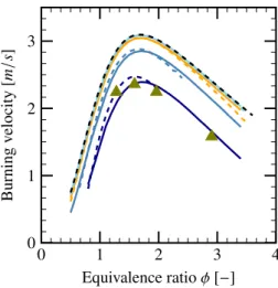
Figure 11: Laminar flame velocity as a function of equivalence ratio. The no spray reference case in the Cosilab code ( ), the calculation results of the Cosilab code with spray of 1.0 × 10⁻⁴( ), 1.5 ×
10−4( ); the results of laminar velocity model of spray 1.0 × 10⁻⁴
( ), 1.5 × 10⁻⁴( ) and 2.0 × 10⁻⁴( ); the experimental results are given in points: spray density 1.0 × 10⁻⁴( ), 1.5 × 10⁻⁴( ) and 2.0 × 10⁻⁴( ).
It can be noted that the water spray has an impor-tant mitigation effect on the laminar flame velocity as the quantity of spray increases. Under spray density of 2.0 × 10⁻⁴, the laminar flame velocity can be decreased from 3.0 m/s to 1.7 m/s for the equivalence ratio φ= 1.7. Both the results of the Cosilab code and those of the LVDEM model can not perfectly fit the experimental re-sults. For the lean mixture (φ < 1), the LVDEM model as well as the the Cosilab code provides lower values for the laminar flame velocity. In [11] the authors emphasize high uncertainty for this part of the measurement.
Comparing the results given by the LVDEM model
and that of the Cosilab code, similar behaviors for the equivalence ratios φ < 1.5 can be noticed. For higher equivalence ratios, no sufficient number of data corre-sponding to the Cosilab code are availbe due to numer-ical instabilities of the calculations. Nevertheless, the burning velocity evolution tendency shows that the Cosi-lab code has underestimated the burning velocity for (φ > 2.0). In contrast, all the estimations for the laminar flame velocity of the LVDEM model are in the vicinity of the experimental results. The most possible reason for this difference comes from the modeling of the evapo-ration rate. It can be noted that the flammability limits are larger in the LVDEM model. In the Cosilab code for water volume fraction 1.0 × 10⁻⁴, the calculation can not converge for the initial gas mixture of equivalence ratio φ > 2. With the LVDEM model, one can calculate the laminar velocity for equivalence ratio up to φ= 3.4.
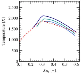
0.1 0.2 0.3 0.4 0.5 0.6 0 500 1,000 1,500 2,000 2,500 XH2[−] T emperature [K ]
Figure 12: Combustion limits for different H2-air compositions
( ); the temperature evolutions given by the laminar flame model are given for spray volume fractions: 1.0 × 10⁻⁴( ), 1.5 × 10⁻⁴
( ) and 2.0 × 10⁻⁴( ).
The combustion limits are important parameters in study of ignition and quenching of the premixed flames. The problem of flammability limits of a combustible gaseous mixture is discussed thoroughly by [34]. The simplified theory [25] states that the flame propagation will not be sustained, or the mixture is not flammable, if:
Tf < Tad RTad Ea + 1 !−1 . (22)
where Tf is the burnt gas temperature in the presence of
heat loss, Tadis the adiabatic burnt gas temperature, R is
the universal gas constant and Eais the global activation
energy of the reaction. The Fig. 12shows the combus-tion limit temperatures, see Equacombus-tion (22), for two dif-ferent global activation energies. The temperature evo-lution inside the flame thickness for hydrogen-air
mix-tures in the presence of the water mists is given in solid lines (water volume fractions 1.0 × 10⁻⁴, 1.5 × 10⁻⁴and 2.0 × 10⁻⁴). According to the equation (22), the mixture is flammable if the temperature is higher than the dashed line.
The global activation energy Ea varies for different
H2-air compositions [35, 36]. The values of Ea
sug-gested by a recent work of [37] have been used in Equa-tion (22). One can see that the combusEqua-tion limits ob-tained using the LVDEM model are close to the theo-retical combustion limits. Moreover, the experiments of [38] provide combustion limits for hydrogen/air/steam mixtures with XH2O = 12% and 0.1 < XH2 < 0.65.
The flammable range estimated by LVDEM is narrower since, in our case, not only the presence of steam but also the evaporation process plays an important role on the flame propagation.
Flame Thickness
Flame thickness is related to the combustion intensity and the flame propagation velocity. According to [31], the most accurate measurement of the flame thickness can be obtained by using the temperature profile. Unfor-tunately, one can not estimate the flame thickness before knowing the temperature profile of the flame propagation for the hydrogen-air mixtures in the presence of water droplets. 1 2 3 4 0.100 0.125 0.150 0.175 0.200 0.225 0.250 0.275 0.300 Equivalence ratio φ [−] Flame thickness [mm ]
Figure 13: Flame thickness evolution as a function of equivalence ratio for different water fraction volumetric: α = 1 × 10⁻⁵( ), α = 5 × 10⁻⁵( ) and α= 8 × 10⁻⁵( ).
From the Fig. 13and Fig. 14, it can be seen that the flame thickness obtained by the LVDEM model behaves like a parabolic function with respect to the equivalence ratio. The minimum of the flame thickness corresponds to the maximal value of the flame velocity. It can be noted that the flame thickness increases with the density of the water spray. Moreover, the Fig.14shows that the
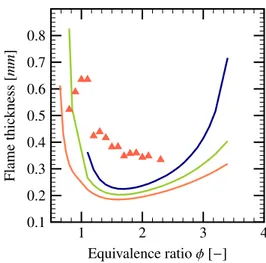
1 2 3 4 0.1 0.2 0.3 0.4 0.5 0.6 0.7 0.8 Equivalence ratio φ [−] Flame thickness [mm ]
Figure 14: Flame thickness evolution as a function of equivalence ratio for different water density on fraction volumetric: α = 1×10⁻⁴( ),
α = 1.5 × 10⁻⁴( ) and α= 2 × 10⁻⁴( ); the results of Cosilab
( ) for α= 1 × 10⁻⁴is given for comparison.
large water density has bigger influence on the lean and rich hydrogen-air mixture. This is due to the fact that the larger thickness of these compositions leads to a more evaporation time and thus a more important influence on the combustion process. The comparison between the LVDEM model and the results of the Cosilab code, ob-tained for D = 6 µm using temperature profiles, shows that the flame thickness estimation has the same order of magnitude. The low combustion limits given by LVDEM model increases with higher droplets volume fraction α. This is due to the increase evaporation rate of the droplets of high volume fraction, which takes in the energy nec-essary to maintain the combustion for lean mixtures.
1 2 3 4 0.15 0.20 0.25 0.30 0.35 Equivalence ratio φ [−] Flame thickness [mm ]
Figure 15: Flame thickness evolution as a function of equivalence ratio for different droplet diameters: 6 µm ( ), 10 µm ( ), 20 µm ( ), 40 µm ( ), α= 1 × 10⁻⁴.
The effects of variation of droplets diameter on the flame thickness are given in Fig. 15. It can be seen that the increase of the droplets diameter while keeping α constant leads to the decrease of the flame thickness. In the other words, it can be deduced that the smaller droplets have more important effects on the flame behav-ior as the droplets surface area increases. The evolution of flame thickness does not vary for droplets of diameter bigger than 20 µm; the two curves corresponding to 20 µm and 40 µm are very similar.
Evaporation Rate
During the flame propagation, the presence of droplets can affect the flame thickness and thus flame velocity mainly due to the evaporation within the flame thick-ness. The evaporation can absorb energy released from the chemical reaction thus leading to a lower burnt gas temperature. However, the evaporation rate depends on the temperature inside the flame thickness. As a con-sequence, these two phenomena are coupled. Determi-nation of the evaporation rate is very important for the estimation of the laminar flame velocity.
0 1 2 3 4 0 1 2 3 4 5 6 7 ·10 −9 Equivalence ratio φ [−] Ev aporation rate [k g /s ]
Figure 16: Evaporation rate of a single droplet as a function of equiv-alence ratio for different droplet diameters: 10 µm ( ), 20 µm ( ), 40 µm ( ), α= 1 × 10⁻⁴.
First, the evaporation during the combustion of one single droplet is investigated using the LVDEM model. The Fig. 16 shows the mass evaporation rate of a sin-gle droplet as a function of equivalence ratio. In the LV-DEM model, a maximal evaporation rate corresponding to the stoichiometric mixture, φ= 1. Away from the sto-ichiometry, the evaporation rate decreases as a result of the decrease of combustion temperature. It can be noted that the evaporation rate increases with the droplet diam-eter for a fixed volume fraction α, since a bigger droplet
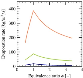
has a larger surface for mass and energy exchange with the gasphase. 0 1 2 3 4 0 100 200 300 400 Equivalence ratio φ [−] Ev aporation rate [k g /m 3/s ]
Figure 17: Evaporation rate of all droplets as a function of equivalence ratio for different droplet diameters: 10 µm ( ), 20 µm ( ), 40 µm ( ), α= 1 × 10⁻⁴.
The Fig. 17 shows the overall evaporation rate of a droplet cloud during the combustion process. In order to highlight the effect of diameter variation, the volume fraction of the liquid phase is fixed as α= 1 × 10⁻⁴for
these calculations. It can be noted that the effect of di-ameter variation on the overall evaporation rate is inverse compared to the single droplet evaporation rate. More precisely, the overall evaporation rate decreases with the increase of the droplet diameter for the same liquid vol-ume fraction. This is due to the fact that, for a fixed volume fraction the liquid-gas interface diminishes with increasing droplet diameter. Thus, it can also be noted from the Fig. 18that the flame velocity increases with bigger droplet diameters.
Effect of Droplet Diameter
During the combustion process, droplet diameter is one of the most important parameters affecting the evap-oration rate. It has been noted that small droplets are easier to evaporate under high temperature, while for the large droplets, it takes more time to evaporate the whole liquid phase, thus leading to a lower evaporation rate. Under the same volumetric fraction of the liquid phase, the droplet diameter has an important influence on the flame velocity. From the Fig. 16, one can see that the bigger droplet has a higher mass evaporation rate. How-ever, the overall evaporation rate is higher for smaller droplets under a fixed volumetric fraction of spray. This can also be seen from the Fig. 18, where the droplets of volume mean diameter 20 µm and 40 µm does not di-minish significantly the flame velocity compared to the case without spray. A critical droplet diameter can be
0 1 2 3 4 0 1 2 3 Equivalence ratio φ [−] Burning v elocity [m /s ]
Figure 18: Evolution of laminar flame velocity as a function of equiv-alence ratio for different droplet diameters; comparison between the Cosilab code 6 µm ( ), 10 µm ( ), 20 µm ( ), 40 µm ( ) and the LVDEM model 6 µm ( ), 10 µm ( ), 20 µm ( ), 40 µm ( ); the experimental results for 6 µm are given in ( ), the reference without spray ( ), α= 1 × 10⁻⁴.
chosen, above which the droplets do not affect the flame velocity. For example, one can take Dc,1 = 35 µm as
the critical diameter, since the flame velocity is reduced only by less than 1.2% for all considered equivalence ra-tios. For smaller droplets, the flame velocity decreases with the decrease of droplet diameters. In Fig. 18, the volumetric fraction of spray is α= 1 × 10⁻⁴.
The comparison between the LVDEM model and the Cosilab code is presented as well in the Fig. 18. Re-sults of the model compare well with those of the Cosilab code, especially for the large droplets. This difference can be explained by the uncertainties of the evaporation model and the estimation of evaporation rate within the flame thickness. Moreover, the experimental results of [11] are well matched by the LVDEM model.
It is noticed in the results of the LVDEM model, for most values of equivalence ratio φ, the droplets of di-ameter 6 µm can not totally evaporate within the flame thickness. Thus, the droplets can penetrate the flame and continue to evaporate in the burnt gas. This is not the case for the very lean or very rich compositions. An-other critical diameter can be chosen Dc,2= 3.9 µm,
be-low which, the droplets can be totally evaporated for all the equivalence ratio values.
4. Conclusions
In this paper, a “Laminar Flame Velocity under Droplet Evaporation Model” (LVDEM) for hydrogen/air mixtures has been developed and validated using the sults of the Cosilab code [20] and the experimental re-sults of [11]. Initially, the hydrogen-air mixture is
sup-posed to be at normal ambient conditions and the water droplet diameter of the order of O(10) µm.
A key ingredient of the LVDEM-model is the droplet evaporation model of [29]. Application of the latter model is necessary in order to determine the amount of liquid water evaporating in the flame zone. Two criti-cal droplet diameters have been considered: (i), Dc,1 =
35 µm above which the droplets do not affect the lami-nar flame velocity for the specific droplet volume frac-tion α = 10−4 and, (ii), D
c,2 = 3.9 µm, below which
the droplets totally evaporate for all equivalence ratios and for droplet volume fractions in the range 0 ≤ α ≤ 2 × 10⁻⁴.
In general, for all considered droplet diameters, the laminar-flame velocity diminishes with increasing water-volume fraction. The laminar flame thickness obtained by the LVDEM-model has the same order of magnitude as that computed with the Cosilab code. In the basis of the presented model, further developments can be envis-aged which would take into account the non-ambient ini-tial mixture conditions in terms of pressure, temperature and gas compositions.
Acknowledgement
This work has been performed with a financial sup-port of the Electricit´e de France (EDF) in the framework of the Generation II&III reactor program, which is grate-fully acknowledged.
Appendix A. The Cosilab Code Algorithm
In the Cosilab code [20], the coupling mechanism of the gaseous and liquid phase is similar to the one pre-sented in [29, 30]. One-dimensional governing equa-tions are solved to obtain a steady solution of a freely propagating, premixed spray flame. Specifically, the gasphase equations are the Eulerian conservation equa-tions of overall mass, species mass, momentum, and energy. The liquid-phase is computed by tracking a stream of droplets in a Lagrangian manner monitoring droplet mass in terms of droplet size, droplet momen-tum or velocity, respectively, and droplet temperature. To relate droplet number density and droplet velocity, the analytical solution of a suitable conservation equa-tion is used [29]. The gasphase and liquid-phase gov-erning equations include phase-exchange terms for liq-uid and gaseous mass, momentum and energy. In the present computations, ideal gas and ideal liquid behavior has been assumed. Due to the assumption of low-Mach-number flow, the pressure could be taken as thermochem-ically constant and hence the gasphase momentum equa-tion could be dropped. The exchange of droplets with the surrounding gas is based on the so-called “stagnant-film
theory”, which incorporates the effect of Stefan flow on the thickness of the droplet-surrounding gaseous bound-ary layer or film. To describe the heat transfer from the gasphase to a liquid drop moving relative to it, radial symmetry is assumed for the drop but, in the Lagrangian sense, an instationary, non-uniform temperature profile inside the drop is considered. The liquid phase is taken as a thin, mono-disperse, single-component spray.
The overall numerical two-phase solution to a spray flame is obtained by coupling the numerical evolution of the two phases. Specifically, the gasphase and liquid-phase governing equations are solved iteratively “in tan-dem” until the numerical solution in either phase has converged.
At a certain iteration step of the overall two-phase tan-dem solution procedure, based on a solution of the Eule-rian gasphase governing equations, the subsequent solu-tion of the Lagrangian liquid-phase governing equasolu-tions is obtained as follows. The vector of primary unknowns is (D(t), vliq(t), Ts(t)), where t is the time, and D, vliq, and
Ts denote the instantaneous diameter, velocity and
sur-face temperature, respectively, of the tracked drop. In the following, the methodology to obtain the droplet surface temperature Ts(t) is summarized. The
remain-ing details of the Lagrangien equations and their solution for D(t) and vliq(t), respectively, are straightforward and
hence for them the reader is referred to Abramzon and Sirignano [29].
To obtain Tsat a particular instant of time,
(1) the molar and mass fluid vapor fractions in the sur-face film of the tracked drop,
XF s= PF s/P, , YF s= XF sMF/
X
i
XiMi, (A.1)
are calculated. Here PF sdenotes the fluid vapor
sat-urated pressure which is evaluated using appropri-ate correlations
PF s= PF s(Ts). (A.2)
(2) the instantaneous average gas-phase properties
ρ, CpF, Cpg, λg, µg, D, Le =
λg
ρgDCpg
, Pr, S c,
in the gas film are calculated – for a definition see the table of contents – using the reference condi-tions given by the so-called one-third rule, viz.,
T = Ts+ 1 3(T∞− Ts), (A.3) YF = YF s+ 1 3(YF∞− YF s). (A.4)
(3) the instantaneous Reynolds number, Re= 2ρ∞|U −
U∞|rs/µg, and the instantaneous Nusselt and
Sher-wood numbers for a non-vaporizing droplet are cal-culated, viz.,
Nu0 = 1 + (1 + Re · Pr)1/3f(Re), (A.5)
S h0 = 1 + (1 + Re · S c)1/3f(Re), (A.6)
where f (Re) = 1 at Re ≤ 1 and f (Re) = Re0.077at Re ≤400.
(4) the instantaneous Spalding mass transfer number, BM, the corresponding diffusional film correction
factor, FM, the modified Sherwood number, S h∗,
and the mass vaporization rate, ˙m, are calculated, viz., BM = YF s− YF∞ 1 − YF s , (A.7) FM = (1 + BM)0.7 ln(1+ BM) BM , (A.8) S h∗ = 2 + (S h0− 2)/FM, (A.9) ˙ m = 2πρgDgrsS h∗ln(1+ BM). (A.10)
(5) the correction factor for the thermal film thickness, FT = F(BT), is calculated using the value of the
heat transfer number, BoldT , from the previous itera-tion or time step.
(6) the modified Nusselt number, Nu∗, the parameter ζ
and the corrected value of the heat transfer number, BT, are calculated, viz.,
Nu∗ = 2 + (Nu0− 2)/FT, (A.11) ζ = CpF Cpg S h∗ Nu∗ ! 1 Le, (A.12) BT = (1 + BM)φ− 1. (A.13)
(7) the heat transferred from the gaseous to the liquid phase, QL= ˙m CpF(Tgas− Ts) BT − l(Ts) , (A.14)
is calculated. Here Tgas denotes the gasphase
tem-perature at the position at which the tracked drop is instantaneously located.
At any discrete time, or time-step, in the Lagrangian solution procedure of the liquid-phase governing equa-tions, the non-dimensional energy equation for the “ef-fective thermal conductivity model” is solved [29], viz.,
(ψ)2∂Z ∂τ =βη ∂Z ∂η + 1 η2 ∂ ∂η(η2 ∂Z ∂η), (A.15)
where Z(η, τ)= (Td(r, t) − T0)/T0is the non-dimensional
drop temperature, ψ(τ) = rs(t)/r0 the instantaneous
non-dimensional drop radius, τ = αLt/r20 the
non-dimensional time, η = r/rs(t) the non-dimensional
ra-dial coordinate, αLthe liquid thermal diffusivity, and β is
proportional to the regression rate of the droplet surfaces, which can be estimated by
β = − 1 4παLρLrs " ˙ m+ 1 ρLCp,L QL # . (A.16)
It is important to note that Eq. (A.15) is solved simulta-neously with the ordinary differential equations that de-scribe the evolution of the liquid phase in terms of the primary liquid-phase dependent variables D(t), vliq(t) and
Ts(t)) discussed above. In particular, at any time t one
has Ts(t)= T0(1+ Z(1, αLt/r20)) where r0= D(0)/2.
Further details of the Lagrangian equations govern-ing D(t), vliq(t) and Ts(t)) are straightforward and can be
found in Abramzon and Sirignano [29].
References
[1] Foissac A, Malet J, Vetrano MR, Buchlin JM, Mimouni S, Feuillebois F, et al. Droplet size and velocity measurements at the outlet of a hollow cone spray nozzle. Atomization Sprays 2011;21:893-905.
https://doi.org/10.1615/AtomizSpr.2012004171.
[2] Joseph-Augustea C, Cheikhravat H, Chaumeixc N, Deria E. On the use of spray systems: An example of R&D work in hydrogen safety for nuclear applications. Int J Hydrogen Energy 2009;34(14):5970-5.
https://doi.org/10.1016/j.ijhydene.2009.01.018
[3] Wingerden KV, Wilkins B, Bakken J, Pedersen G. The influence of water sprays on gas explosions. Part 2: mitigation. J Loss Prev Process Ind 1995;8(2):61-70.
https://doi.org/10.1016/0950-4230(95)00007-N.
[4] Pilch M, Erdman CA. Use of breakup time data and velocity history data to predict the maximum size of stable fragments for acceleration-induced breakup of a liquid drop. Int J Multiphase FLow 1987;13(6):741-57.
https://doi.org/10.1016/0301-9322(87)90063-2.
[5] Chou W-H, Hsiang L-P, Faeth GM. Temperal properties of drop breakup in the shear breakup regime. Int J Multiphase FLow 1997;23(4):651-69.
https://doi.org/10.1016/S0301-9322(97)00006-2.
[6] Meng JC, Colonius T. Numerical simulation of the aerobreakup of a water droplet. J Fluid Mech 2018;835:1108-35.
https://doi.org/10.1017/jfm.2017.804.
[7] Sapko MJ, Furno AL, Kuchta JM. Quenching methane-air ignitions with water sprays. Bureau of Mines Report of Investigations. RI 8214; 1977.
[8] Zalosh RG, Bajpai SN. Water fog inerting of hydrogen-air mixtures. Proc. 2nd Int Conf on the Impact of Hydrogen on Water Reactor Safety. New Mexico, USA; 1982.
[9] Boech LR, Kink A, Oezdin D, Hasslberger J, Sattelmayer T. Influence of water mist on flame acceleration, DDT and detonation in H2-air mixtures. Int J Hydrogen Energy
2015;40(21):6995-7004.
https://doi.org/10.1016/j.ijhydene.2015.03.129.
[10] Holborn PG, Battersby P, Ingram JM, Averill AF, Nolan PF. Modelling the effect of water fog on the upper flammability limit of hydrogen-oxygen-nitrogen mixtures. Int J Hydrogen Energy
2013;38(16):6896-903.
https://doi.org/10.1016/j.ijhydene.2013.03.091.
[11] Ingram JM, Averill AF, Battersby PN, Holborn PG, Nolan PF. Suppression of hydrogen-oxygen-nitrogen explosions by fine water mist: part 1, burning velocity. Int J Hydrogen Energy 2012;37(24):19250-7.
https://doi.org/10.1016/j.ijhydene.2012.09.092. [12] Gai G, Kudriakov S, Hadjadj A, Studer E, Thomine O.
Modeling of pressure loads during a premixed hydrogen combustion in the presence of water spray. Int J Hydrogen Energy 2019;44(10):4592-607.
https://doi.org/10.1016/j.ijhydene.2018.12.162. [13] FLACS V 10.2. User’s Manual. GexCon AS; 2014. [14] Keenan JJ, Makarov DV, Molkov VV. RayleigheTaylor
instability: modelling and effect on coherent deflagrations. Int J Hydrogen Energy 2014;39(35):20467-73.
https://doi.org/10.1016/j.ijhydene.2014.03.230. [15] Bauwens CR, Chaffee J, Dorofeev SB. Vented explosion
overpressures from combustion of hydrogen and hydrocarbon mixtures. Int J Hydrogen Energy 2011;36(3):2329-36. https://doi.org/10.1016/j.ijhydene.2010.04.005. [16] Velikorodny A, Studer E, Kudriakov S, Beccantini A.
Combustion modeling in large scale volumes using
EUROPLEXUS code. J Loss Prev Process Ind 2015;35:104-16. https://doi.org/10.1016/j.jlp.2015.03.014.
[17] Dahoe AE. Laminar burning velocities of hydrogen-air mixtures from closed vessel gas explosions. J Loss Prevent Proc 2015;18(3):152-66. https://doi.org/10.1016/j.jlp.2005.03.007. [18] Konnov AA. Remaining uncertainties in the kinetic mechanism
of hydrogen combustion. Combust Flame 2008;152(4):507-28. https://doi.org/10.1016/j.combustflame.2007.10.024.
[19] Ballal DR, Lefebvre AH. Flame propagation in heterogeneous mixtures on fuel droplets, fuel vapor and air. 18th Symposium (International) on Combustion. The Combustion Institute; 1981. https://doi.org/10.1016/S0082-0784(81)80037-9.
[20] Cosilab (V 4.1) Software. User manual two-phase flames. www.rotexo.com. 2018.
[21] Neophytou A, Mastorakos E. Simulations of laminar flame propagation in droplet mists. Combust Flame
2009;156(8):1627-40.
https://doi.org/10.1016/j.combustflame.2009.02.014. [22] Grosseuvres R, Comandini A, Bentaib A, Chaumeix N.
Combustion properties of H2/N2/O2/steam mixtures.
Proceedings of the Combustion Institute 2019;37(2):1537-46. https://doi.org/10.1016/j.proci.2018.06.082.
[23] Satija A, Huang X, Panda PP, Lucht PR. Vibrational CARS thermometry and one-dimensional simulations in laminar H2/air
counter-flow diffusion flames. Int J Hydrogen Energy 2015;40(33):10662-72.
https://doi.org/10.1016/j.ijhydene.2015.06.150.
[24] Connaire MO, Curran HJ, Simmie JM, Pitz WJ, Westbrook CK. A comprehensive modeling study of hydrogen oxidation. Int J Chem Kinet 2004;36(11):603-22.
https://doi.org/10.1002/kin.20036.
[25] Williams FA. Combustion Theory. 2nd ed. CRC Press; 1994. [26] R.J. Kee, M.E. Coltrin, P. Glarborg, H. Zhu. Chemically
Reacting Flow: Theory, Modeling, and Simulation. 2nd ed. Wiley; 2017.
[27] Koroll GW, Kumar RK, Bowles EM. Burning velocities of hydrogen-air mixtures. Combust Flame 1993;94(3):330-40. https://doi.org/10.1016/0010-2180(93)90078-H.
[28] Szab´o T, Y`a˜nez J, Kotchourko A, Kuznetsov M, Jordan T. Parameterization of laminar burning velocity dependence on pressure and temperature in hydrogen/air/steam mixtures. Combust Sci Technol 2012;184:1427-44.
https://doi.org/10.1080/00102202.2012.690253.
[29] Abramzon B, Sirignano WA. Droplet vaporization model for spray combustion calculations. Int J Heat Mass Transfer
1988;32(9):1605-18.
https://doi.org/10.1016/0017-9310(89)90043-4.
[30] Sirignano WA. Fluid dynamics and transport of droplets and sprays. 2nd ed. Cambridge University Press; 2010.
[31] Poinsot T, Veynante D. Theoretical and numerical combustion. Philadelphia: Edwards; 2001.
[32] Gaydon AG, Wolfhard HG. Flames: their structure, radiation and temperature. 4th ed. London: Chapman and Hall; 1979. [33] Ingram JM. Private communication.
[34] Luangdilok W, Bennett RB. Fog inerting effects on hydrogen combustion in a PWR ice condenser containment. J Heat Transfer 1995;117(2):502-7. https://doi.org/10.1115/1.2822550. [35] Travis JR. A heat, mass, and momentum transport model for
hydrogen diffusion flames in nuclear reactor containments. Nucl Eng Des 1987;101:149-166.
[36] Gavrikov AI, Bezmelnitsyn AV, Leliakin AL, Dorofeev SB. Extraction of basic flame properties from laminar flame speed calculations. 23 thInternational Colloquium on the Dynamics of Explosions and Reactive Systems. 2001.
[37] Yanez J and Kuznetsov M. An analysis of flame instabilities for hydrogen–air mixtures based on Sivashinsky equation. Physics Letters A 2016;380(33):2549-60.
https://doi.org/10.1016/j.physleta.2016.05.048.
[38] Cheikhravat H. Etude exp´erimentale de la combustion de l’hydrog`ene dans une atmosph`ere inflammable en pr´esence de gouttes d’eau. PhD. Thesis. Universit´e d’Orl´eans; 2009.
![Figure 8: The burner and mist generation system scanned from [11].](https://thumb-eu.123doks.com/thumbv2/123doknet/13577999.421782/10.892.168.394.110.335/figure-burner-mist-generation-scanned.webp)