HAL Id: cea-02284855
https://hal-cea.archives-ouvertes.fr/cea-02284855
Submitted on 3 Jun 2021
HAL is a multi-disciplinary open access archive for the deposit and dissemination of sci-entific research documents, whether they are pub-lished or not. The documents may come from teaching and research institutions in France or abroad, or from public or private research centers.
L’archive ouverte pluridisciplinaire HAL, est destinée au dépôt et à la diffusion de documents scientifiques de niveau recherche, publiés ou non, émanant des établissements d’enseignement et de recherche français ou étrangers, des laboratoires publics ou privés.
To cite this version:
X. Kong, Olivier Asserin, S. Gounand, P. Gilles, J.-M. Bergheau, et al.. 3D finite element simula-tion of TIG weld pool. IOP Conference Series: Materials Science and Engineering, IOP Publishing, 2012, MCWASP XIII - International Conference on Modeling of Casting, Welding and Advanced Solidification Processes, 33, pp.012025. �10.1088/1757-899X/33/1/012025�. �cea-02284855�
3D finite element simulation of TIG weld pool
X Kong1,2,3 , O Asserin1 , S Gounand1 , P Gilles2 , JM Bergheau3 and M Medale4 1CEA, DEN, DANS, DM2S, F-91191 Gif-sur-Yvette, France 2
AREVA NP, Paris La D´efense, France 3
LTDS, Ecole Nationale d’Ing´enieurs de Saint-Etienne, France 4
Ecole Polytechnique Universitaire de Marseille, Marseille, France E-mail: [email protected], [email protected]
Abstract. The aim of this paper is to propose a three-dimensional weld pool model for the
moving gas tungsten arc welding (GTAW) process, in order to understand the main factors that limit the weld quality and improve the productivity, especially with respect to the welding speed. Simulation is a very powerful tool to help in understanding the physical phenomena in the weld process. A 3D finite element model of heat and fluid flow in weld pool considering free surface of the pool and traveling speed has been developed for the GTAW process. Cast3M software is used to compute all the governing equations. The free surface of the weld pool is calculated by minimizing the total surface energy. The combined effects of surface tension gradient, buoyancy force, arc pressure, arc drag force to drive the fluid flow is included in our model. The deformation of the weld pool surface and the welding speed affect fluid flow, heat flow and thus temperature gradients and molten pool dimensions. Welding trials study is presented to compare our numerical results with macrograph of the molten pool.
1. Introduction
Gas tungsten arc welding (GTAW) is a widely used technique for joining steel in nuclear industry where the weld quality must be ensured. An increased productivity of welding would have a very important economic impact for the industrial sector. Although GTAW is already a very efficient process, it can be improved, especially with respect to the welding speed. The aim of this paper is to propose a three-dimensional weld pool model for the moving GTAW process, in order to understand the main factors that limit the weld process and improve the productivity. Simulation is very helpful in understanding the physical phenomena in the weld pool and optimizing the process. In the recent years, many research dealing with the simulation of welding processes have been carried out and great progress has been made. Tanaka [1] took into account tungsten cathode, arc plasma and anode in a 2D axisymmetric unified model, but the deformation of the free surface of weld pool isn’t taken into account. Debroy and al. [2] developed a 3D model with a moving heat source but the Marangoni coefficient is assumed constant. Lu and al. [3] developed a coupled model in 2D axisymmetric with the interface deformation, and the weld pool shape calculated agrees better with the experiment than the model without the free surface. Wu and al. [4] studied both front and back side deformations of fully penetrated GTAW weld pool surfaces, they gave a detailed derivation of the partial differential equation for predicting both surface deformation. Kim and Na [5] presented a 3D quasisteady heat and fluid flow analysis for the moving heat source of the gas metal arc welding
(GMAW) process with the free surface, and Hu and al. [6] modelled the transient weld pool dynamics under the periodic impingement of filler droplets. However, there is no impingement of droplets in GTAW which is very different from GMAW. Most of the present mathematical model are realised with the method of finite volume or finite difference, nowadays there is a increasing tendency to apply finite element methods. Among the reasons can be ability of the finite element method to handle complex coupled thermomechanical mechanisms with various and complex boundary conditions.
In this paper, a 3D finite element model considering free surface, moving source and temperature dependence of thermophysical properties for the GTAW is performed. The free surface profile is calculated by minimizing the total energy of the surface, the arc pressure, the arc drag force and the heat flux are given by a 2D axisymmetric arc plasma unified model [7]. The continuity equation, momentum equation and energy conservation equation are solved together by the Cast3M software [8], until a steady solution is found. The calculated GTAW weld bead geometry shows favourable agreement with experimental results.
2. Mathematical model
The 3D model of the welding pool with taking into account the traveling speed and the free surface is shown below. The assumptions are the following:
• a stationary solution is sought;
• the liquid metal is considered a Newtonian fluid;
• it is assumed that the flow of liquid metal is not turbulent; • it is assumed that the Boussinesq approximation can be used;
• the speed of the power source vs is assumed constant and the equations are solved in a
reference frame moving with the source;
• in the fluid phase, the equations of conservation of mass, momentum and energy are solved, only the energy equation remains in the solid phase.
The unknowns of the problem are:
- v velocity in the fluid phase in the reference frame linked to the source (v = vs in the solid
phase);
- p, the pressure in the fluid phase;
- h and T , the enthalpy and the temperature. 2.1. Continuity equation
In the weld pool region, the continuity equation for an incompressible fluid holds:
∇.v = 0 (1)
where v is the velocity of the fluid in the weld pool. 2.2. Momentum equation
The flow of the liquid metal in the weld pool conforms to the following equations:
ρ(∇v).(v − vs) = −∇p + ∇.µ(∇v + ∇Tv) + fBou+ fExt (2)
ρ = ρ0+
∂ρ
∂T(T − Tref) (3)
where vs is the velocity of the power source, p is the hydrostatic pressure, µ is the viscosity,
the buoyancy force: fBou= ρ0gβ(T − Tref)uz where ρ0 is the mass density at the temperature
Tref = 1730K and uz is a vertical unit vector, the force of extinction speed: fExt= −AFs(T )v
avec A = 1012
>> 1 where Fs is the solid fraction [9].
The boundary conditions are :
v= vs at ∂Ωs/l (4)
v.n = 0 at ∂Ωf (5)
(µ(∇v + ∇Tv).n).t = fMarangoni.t + fdrag.t at ∂Ωf (6)
where ∂Ωs/l represent the liquid/solid interface and ∂Ωf is the free surface, n and t are the
normal and the tangential direction to surface, fdrag is the arc drag force which will be given in
the next subsection as a kind of surface source, fMarangoni =
∂γ ∂T∇T , ∂γ ∂T is given by ∂γ ∂T = −Ar−RΓsln(1 + k1asexp(−∆H0/RT )) − k1asΓs∆H0exp(−∆H0/RT ) (1 + k1asexp(−∆H0/RT ))T (7) where γm is the surface tension at melting temperature, Ar is the opposite of dγ/dT for a pure
FeS alloys, R is the gas constant, Γsis the surface excess at saturation, asis the activity of sulfur,
∆H0 is the standard heat of adsorption, and k1 is a constant related to entropy of segregation
[10].
2.3. Energy conservation equation
The energy conservation can be written as follows :
ρcp(∇h).(v − vs) = ∇.λ∇T (8)
where cp is the specific heat, h is the enthalpy, λ is the thermal conductivity.
The boundary conditions are :
h = h0 on ∂Ωin (9)
λ∇T.n = 0 on ∂Ωout (10)
λ∇T.n = qr+ qc+ qs on ∂Ωsurf (11)
where ∂Ωin and ∂Ωout are the surface entering and leaving of the calculated domain, ∂Ωsurf
represent the other surfaces of the workpiece. The convective heat loss is qc = −hc(T − T∞),
and the radiative loss is qr= −ǫσ(T4−T∞4), qs is the heat flux which will be given in the next
subsection.
2.4. The free surface
The surface depression will form a shape which minimizes the total energy. The total energy to be minimized includes the surface energy due to the change in area of the pool surface, the potential energy in the gravitational field and the the work performed by the arc pressure displacing the pool surface [4].
γ
R = ρ0gϕ + Pa+ λ (12)
R and ϕ are the radius curvature and the elevation, ϕ is the elevation, γ represent the surface tension which is a variable in function of temperature. λ is the Lagrange multiplier which can be determined from keeping constant volume of the workpiece. The surface tension depends on temperature, for FeS alloys, following the model presented by Sahoo et al [10] γ is :
γ = γm−Ar(T − Tf) − RT Γsln(1 + k1asexp(−∆H0/RT )) (13)
2.5. Treatment of latent heat
In order to treat phase change in the weld pool liquid/solid interface, the method of V.R. Voller [9], [11] is used. The total enthalpy H is represented as the integral of heat capacity with respect to temperature and can be written as follows:
H(T ) = Z T
Tref
ρcp(T )dT (14)
where ρcp(T ) is the volumetric heat capacity which depends on temperature, and where Tref
is a reference temperature. In the industrial application, it is assumed that the phase change takes place over a finite interval [Ts, Tl], the enthalpy function can be given by:
H(t) = RT Trefρcs(T )dT, f or T ≤ Ts, RTs Trefρcs(T )dT + RT Tsρ ∂L ∂TdT, f or Ts< T ≤ Tl, RTs Trefρcs(T )dT + ρL + RT Tlρcl(T )dT, f or T > Tl, (15)
where Ts and Tl are the solidus and liquidus temperatures, and ρcs(T ) and ρcl(T ) are the
temperature dependent volumetric heat capacities, L is latent heat. 2.6. Thermophysical properties
The temperature dependance of thermophysical properties is considered in this paper instead of supposing constant values. The thermophysical properties in solid and liquid (cp, h, ρ, λ, µ, β)
for the material 316L steel are taken from Kim [12], for ∂γ
∂T and γ, the formula of Sahoo [10] is used. Other thermophysical properties and parameters used in this paper are summarized in Table 1.
2.7. Determination of surface sources
The study focusses on the weld pool behaviour, classical Gaussian distribution for the heat flux and arc pressure could have been used. However, this would have affected the simulation predictive capabilities, because the parameters of Gaussian distribution are not related to the welding operating parameters. So an hybrid 2D-3D approach is performed: the boundary conditions used in the three-dimensional weld pool model (heat flux, arc pressure and arc drag force) are calculated with a 2D axisymmetric arc plasma model [7]. The present GTAW experiment are carried out under following conditions: 316L steel workpiece with dimensions 200 × 50 × 6 mm3
, the welding current is 150 A, the arc voltage is 10 V, the arc length is 2 mm, the welding speed is 15 cm/min, the shielding gas is argon with flow rate 20 l/min, the tungsten electrode is of diameter 3.2 mm with tip angle 30◦
. Then these welding conditions are used in the 2D axisymmetric arc plasma model, figures 1, 2 and 3 show the 2D-computed heat flux, arc pressure and arc drag force which will be used in the 3D finite element weld pool model. 3. Numerical model
The finite element method is used to discretize the equations of the problem. Quadratic and linear finite elements are used for the variable v and for the variables p, h and T . The method of weighted residuals is applied to seek the cancellation of integral terms associated with our problem. The coupling between the problem of fluid flow and heat transfer is taken into account with a suitable algorithm for solving the uncoupled finite element formulation (Table 2). The system of equations to be solved is non-linear, it is found that the thermal non-linearities are resolved fairly with the enthalpy formulation used, but the non-linearities associated with the
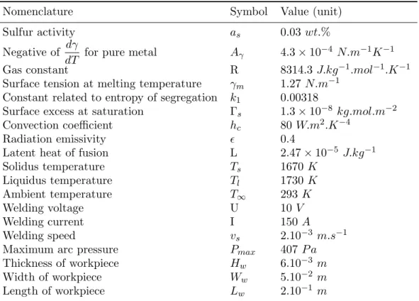
Table 1. Thermophysical properties of 316 stainless steel and welding conditions
Nomenclature Symbol Value (unit)
Sulfur activity as 0.03 wt.%
Negative of dγ
dT for pure metal Aγ 4.3 × 10
−4 N.m−1 K−1 Gas constant R 8314.3 J.kg−1 .mol−1 .K−1
Surface tension at melting temperature γm 1.27 N.m−1
Constant related to entropy of segregation k1 0.00318
Surface excess at saturation Γs 1.3 × 10⁻⁸ kg.mol.m−2
Convection coefficient hc 80 W.m2.K−4
Radiation emissivity ǫ 0.4
Latent heat of fusion L 2.47 × 10⁻⁵
J.kg−1 Solidus temperature Ts 1670 K Liquidus temperature Tl 1730 K Ambient temperature T∞ 293 K Welding voltage U 10 V Welding current I 150 A Welding speed vs 2.10−3 m.s−1
Maximum arc pressure Pmax 407 P a
Thickness of workpiece Hw 6.10−3 m Width of workpiece Ww 5.10−2 m Length of workpiece Lw 2.10−1 m X(m) P(Pa) 0.00 0.10 0.20 0.30 0.40 0.50 0.60 0.70 0.80 0.90 1.00 x1.E−2 0.00 0.50 1.00 1.50 2.00 2.50 3.00 3.50 4.00 4.50 x1.E2
Figure 1. Radial evolution of arc pressure [7]. X(m) Ft(Pa) 0.00 0.10 0.20 0.30 0.40 0.50 0.60 0.70 0.80 0.90 1.00 x1.E−2 0.00 5.00 10.00 15.00 20.00 25.00 30.00 35.00 40.00 45.00 50.00
Figure 2. Radial evolution of arc drag force [7].
X(m) Q(W/m2) 0.00 0.10 0.20 0.30 0.40 0.50 0.60 0.70 0.80 0.90 1.00 x1.E−2 0.00 1.00 2.00 3.00 4.00 5.00 6.00 7.00 8.00 x1.E7
Figure 3. Radial evolution of heat flux [7].
fluid are generally more difficult to treat, for example the non-linearities due to the convective term and the phase change. The strategy is as follows: at the beginning of the calculation, the driving force fMarangoni is initialized to zero, the thermal problem is solved. When there is a
convergence on the unknowns of the non-linear problem, the intensity of the driving force fα
is increased with a coefficient α. And for improving the convergence, the convection terms are upwinded using a Streamline-Diffusion method.
Table 2. Algorithm for solving the non-linear problem Initial condition: (v, p, h, T, α)0
at i = 0 Repeat
i = i + 1
Determination of the fluid mesh
Calculation of the increments δv, δp and update (v, p)i = (v, p)i−1+ (δv, δp)
Calculation of the free surface profile, update ϕi = ϕi−1+ δϕ and mesh movement Calculation of the increment δh , update hi= hi−1+ δh and calculation Ti = T (hi) when δinc= (δv, δp, δh) < δconv, α = min(α ∗ fα, 1)
until δinc< δconv and α = 1
4. Results and discussion
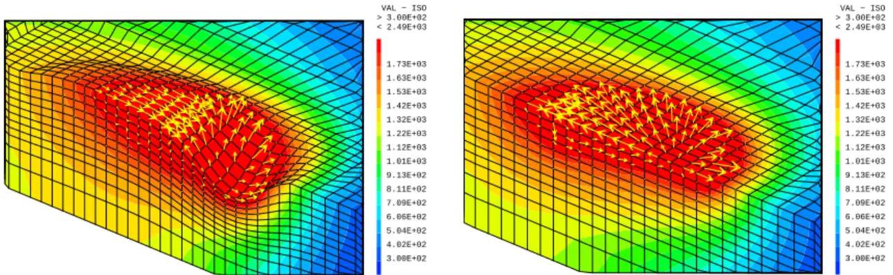
Figure 4 show the temperature and velocity field with heat transfer and fluid flow model taking into account the free surface, as shown in this figure, the base metal ahead of the heat source has not yet melted. The weld top surface of the region directly under the heat source is strongly deformed under the arc pressure, the molten metal is pushed to the rear part of the weld pool by combined effect of all the driving forces. As the monitoring location moves away from the heat source, the weld pool surface shows less depression because of reduction of arc pressure. Furthermore, the accumulation of the liquid metal in the rear part is clearly shown.
VAL − ISO > 3.00E+02 < 2.49E+03 3.00E+02 4.02E+02 5.04E+02 6.06E+02 7.09E+02 8.11E+02 9.13E+02 1.01E+03 1.12E+03 1.22E+03 1.32E+03 1.42E+03 1.53E+03 1.63E+03 1.73E+03
Figure 4. Calculated weld pool with considering free surface.
VAL − ISO > 3.00E+02 < 2.49E+03 3.00E+02 4.02E+02 5.04E+02 6.06E+02 7.09E+02 8.11E+02 9.13E+02 1.01E+03 1.12E+03 1.22E+03 1.32E+03 1.42E+03 1.53E+03 1.63E+03 1.73E+03
Figure 5. Calculated weld pool without considering free surface.
4.1. Weld temperature and fluid velocity field
In order to understand the influence of the free surface on the weld temperature and fluid velocity, two simulations are performed using the experimental welding parameters: one takes into account the free surface in our model (figure 4) and the other one doesn’t (figure 5). Table 3 summarize the calculated weld pool characteristics, the maximal temperature in the case without free surface is 220 K higher than the one with free surface. When the free surface is taken into account, the fluid velocity is increased by the depression of free surface, and it will bring more heat energy to the rear part of weld pool, increase the volume of the weld pool, reduce the maximal temperature and finally change the isothermals.
The figures 6 and 7 show the temperature field of these two cases at the bottom surface of workpiece. In front of the heat source, the difference in the isothermals is quite small, on
the other hand, the isothermals are very different behind the heat source. The isothermals are elongated for the case with free surface than the one with fixed surface, and the temperature difference exceeds 100 K in a huge area. Therefore, it is important to consider the free surface in the simulation of GTAW process.
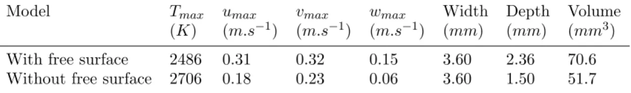
Table 3. Weld pool characteristics in the models with and without free surface
Model Tmax umax vmax wmax Width Depth Volume
(K) (m.s−1
) (m.s−1
) (m.s−1
) (mm) (mm) (mm3
)
With free surface 2486 0.31 0.32 0.15 3.60 2.36 70.6
Without free surface 2706 0.18 0.23 0.06 3.60 1.50 51.7
With free surface
VAL − ISO > 3.00E+02 < 1.35E+03 5.50E+02 6.00E+02 6.50E+02 7.00E+02 7.50E+02 8.00E+02
Without free surface
Figure 6. Calculated temperature field at the bottom surface of workpiece for the case without and with considering free surface. VAL − ISO >−7.58E−02 < 1.36E+02 5.3 12. 18. 25. 31. 38. 44. 51. 57. 63. 70. 76. 83. 89. 96. 1.02E+02 1.09E+02 1.15E+02 1.22E+02 1.28E+02 1.35E+02
Figure 7. Difference of calculated temperature field at the bottom surface of workpiece with and without considering free surface.
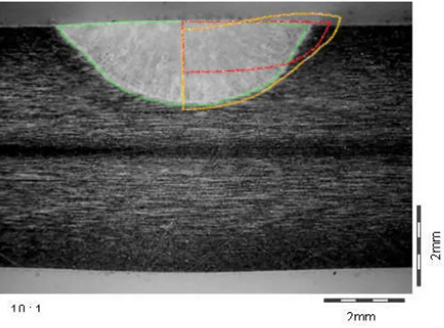
4.2. Weld bead geometry
The crosssection macrograph of welded joint is shown in figure 8, which also indicate the calculated weld bead shape by the models with and without free surface. As shown in this figure, the width of weld pool with a flat surface is wider than experiment and the depth is smaller, on the other hand, the shape of the weld and the penetration are better predicted when we take account into the free surface. As shown in figure 4 and figure 5, fluid flow and heat are taken away from the center of weld pool to the edge, so the deepest position of the weld pool is not just below the moving heat source, but after it because of the convection. When the surface is free, the front part of weld pool is strongly depressed by the arc pressure, so the fluid velocity at the surface is bigger and more fluid flow and heat are taken to the back part of weld pool which lead to a deeper penetration. For this experiment, the heat transfer and fluid flow model with free surface is better to predict the weld bead geometry.
5. Conclusion
A three-dimensional model of heat transfer and fluid flow has been presented in this paper, which can calculate the temperature and velocity field, predict the weld pool shape and size.
Figure 8. Experimental (green line) and calculated weld pool shape (yellow line model with free surface and red line model without free surface.
The following conclusions can be given:
(1) The model solves the continuity, momentum conservation, and energy conservation equations with taking account into the free surface and phase change, and a steady solution for the temperature, velocity field and the free surface of weld pool can be found.
(2) Taking account into the free surface in the simulation of weld pool has a great influence on the fluid velocity, the isothermals and the dimensions of the weld bead.
(3) Experimental results show that there is a good agreement between the simulated profile of weld bead by our 2D-3D approach model and the experimental one.
6. Reference
[1] Tanaka M, Terasaki H, Ushio M and Lowke J 2002 Metallurgical and Materials Transactions A 33 2043–2052 [2] Mundra K and Debroy T 1996 Numerical Heat Transfer 29 115
[3] Lu F, Tang X, Yu H and Yao S 2006 Journal of Applied Physics 35 458 [4] Wu C, Chen J and Zhang Y 2007 Computational Materials Science 39 635–642 [5] Kim J and Na S 1994 ASME J. Eng. Ind 116 78–85
[6] Hu J, Guo H and Tsai H 2008 International Journal of Heat and Mass Transfer 51 2537
[7] Brochard M 2008 A unified model of gas tungsten arc welding including electrode, arc plasma and molten
pool Ph.D. thesis Commissariat `a l’Energie Atomique, France
[8] Cast3M 2008 http ://www-cast3m.cea.fr
[9] Brent A, Voller V and Reid K 1988 Numerical Heat Transfer 13 297–318
[10] Sahoo P, Debroy T and McNallan M 1988 Metallurgy and Materials Transactions B 19 483–491 [11] Nedjar B 2002 Computers and Structures 80 9–21
[12] Kim C 1975 Thermophysical properties of stainless steels Master’s thesis Argonne national laboratory