Analogic for code estimation and detection

£9

Analogic for Code Estimation and Detection

by

Xu Sun

Submitted to the Program in Media Arts and Sciences,

School of Architecture and Planning

in partial fulfillment of the requirements for the degree of

Master of Science in Media Arts and Sciences

at the

MASSACHUSETTS INSTITUTE OF TECHNOLOGY

September 2005

@

Massachusetts Institute of Technology 2005. All rights reserved.

A uthor ...

Program in Media Arts and Sciences,

School of Architecture and Planning

,1,) '-n

71

August 5, 2005

Certified by

_{. . . .}

Neil Gershenfeld

Associate Professor

Thesis Supervisor

A ccepted by ...

... z... ... ....

.

....

Chairman, Departmental Committee on Graduate Students

SEP 2 6 2005

LIBRARIES

ROTCH

Analogic for Code Estimation and Detection

by

Xu Sun

Submitted to the Program in Media Arts and Sciences, School of Architecture and Planning

on August 5, 2005, in partial fulfillment of the requirements for the degree of

Master of Science in Media Arts and Sciences

Abstract

Analogic is a class of analog statistical signal processing circuits that dynamically solve an associated inference problem by locally propagating probabilities in a message-passing algorithm [29] [15]. In this thesis, we study an exemplary embodiment of analogic called Noise-Locked Loop(NLL) which is a pseudo-random code estimation system. The previous work shows NLL can perform direct-sequence spread-spectrum acquisition and tracking functionality and promises orders-of-magnitude win over dig-ital implementations [29].

Most of the research [30] [2] [3] has been focused on the simulation and implemen-tation of probability represenimplemen-tation NLL derived from exact form message-passing algorithms. We propose an approximate message-passing algorithm for NLL in log-likelihood ratio(LLR) representation and have constructed its analogic implementa-tion. The new approximate NLL gives shorter acquisition time comparing to the exact form NLL. The approximate message-passing algorithm makes it possible to construct analogic which is almost temperature independent. This is very useful in the design of robust large-scale analogic networks.

Generalized belief propagation(GBP) has been proposed to improve the computa-tional accuracy of Belief Propagation [31] [32] [33]. The application of GBP to NLL promises significantly improvement of the synchronization performance. However, there is no report on circuit implementation. In this thesis, we propose analogic cir-cuits to implement the basic computations in GBP, which can be used to construct general GBP systems.

Finally we propose a novel current-mode signal restoration circuit which will be im-portant in scaling analogic to large networks.

Thesis Supervisor: Neil Gershenfeld Title: Associate Professor

-. .

<

&

e

~

n

W

i'-

o

i:=

w

d

a

s

i e

m-Analogic for Code Estimation and Detection

by

Xu Sun

Submitted to the Program in Media Arts and Sciences in partial fulfillment of the requirements for the degree of

Master of Science in Media Arts and Sciences at the

MASSACHUSETTS INSTITUTE OF TECHNOLOGY

September 2005 Thesis A dvisor... Thesis Reader .... Thesis Reader ...

...

Rahul Sarpeshkar Robert J. Shillman Associate Professor Department of Electrical Engineering and Computer Science Massachusetts Institute of Technology

... .... I ... ... Benjamin Vigoda Research Scientist Mitsubishi Electric Research Laboratories (MERL)

-... .r. - . -, .--.-s--:,' : -7 :2 -"

e

Acknowledgments

I realize that I have received invaluable help from so many remarkable people during the thesis study.

Thank you to my advisor Neil Gershenfeld for his great insight to the study of ana-logic. Thank you for providing us such a free academic atmosphere in Physics and Media Group, where his encouragement to our crazy ideas and tolerance to sometime not-so-good results is always like from a generous father to his kids. Thank you for his directing of Center for Bits and Atoms, which greatly expands our vision and pro-vides me good opportunity to work with excellent people around the campus. Thank you for all his practical support, encouragement, and guidance through out my first two years in MIT, which are also my first two years in this country.

Thank you to my thesis reader Rahul Sarpeshkar! His seeking spirit in the research, everlasting curiosity toward hard problems, great physical intuition, and academic discipline sets up a great pattern to me. Thank you for his excellent knowledge and creativity in analog circuit design, which inspires my interests in this area. Thank you for his constant care for my research. Thank you for giving me the access to his lab where I learned a lot on circuit testing.

Thank you to my thesis reader Benjamin Vigoda! The work in this thesis has largely built on the foundation that he layed in his master and Ph.D. research. Thank you for his willingness to spend so many hours with me whenever I asked him questions. Thanks for his encouragement whenever I made some progress.

Thank you to Prof. Michael Perrott for his excellent simulator CppSim. Great part of the system level simulation in this thesis is done by it. Also thanks to him for sharing his insights on possible applications of noise-locked loop.

Thank you to Yael Maguire for sharing me your knowledge in electronics and giving me many valuable suggestions on my startup. Thank you to Ben Recht for educating me on mathematical optimization and his eagerness to know my progress.Thank you to Jason for the discussion on normalization problem. Thank you to Manu for an-swering me all the detailed questions on thesis preparation and writing and printing.

Thank you to Amy on helping me fabricate in the shop any thing I want. Thank you to Ara.

I owe a great thank you to Soumyajit Mandal. He answered so many of my questions on circuit design. He generously gave me his own lab bench for my final testing. Also thanks for his proofreading my thesis. Thank youn to Scott Arfin for helping me set up GPIB on my laptop. Thank you to Michael Baker for his suggestions which improved my circuit a lot. Thank you to Piotr Mitros for teaching me analog circuit troubleshooting techniques and spending so many late hours in the lab with me. Thanks to Linda Peterson and Pat Sokaloff for taking care of us graduate students. Thank you to Susan Murphi-Bottari, Mike Houlihan, Kelly Maenpaa for keeping PHM running smoothly.

Thank you to my Mom and Dad for their love that I can feel it even when I am on the other side of the earth. Thank you to my wife Grace for all her love, care, encouragement during the hard time of research.

Thank you to my Lord Jesus Christ. Thank You for Your life in me. -..- K- i - 0 -Qlsm 4 I - 1 1--.- -- l- I . -- -I, - ---

-Contents

1 Introduction 21

1.1 Review of Previous Work . . . . 22

1.2 M otivation . . . . 23

1.3 Contribution . . . . 24

1.4 Thesis Outline . . . . 26

2 Background Information 27 2.1 Phase-Locked Loop . . . . 28

2.2 Spread Spectrum Systems . . . . 30

2.3 Message-Passing Algorithms . . . . 34

3 LFSR Synchronization: From Scalar NLL to Vector NLL 39 3.1 LFSR Synchronization as Maximum Likelihood Estimation . . . . 41

3.2 Exact Form Scalar NLL . . . . 44

3.2.1 Probability Representation . . . . 45

3.2.2 Log-Likelihood Ratio(LLR) Representation . . . . 46

3.3 Approximate Scalar NLL in Log-Likelihood Ratio(LLR) Representation 46 3.3.1 Multiplier Approximation . . . . 47

3.3.2 Simulation of Exact Form and Approximate Scalar NLLs . . . 49

3.4 First-Order Markov Structured Vector NLL . . . . 57

3.5 LFSR Synchronization by Iterative Detection . . . . 62

4 Analogic Implementation of NLLs 65

4.1 Fundamental Circuit ... ... 65

4.1.1 Static Translinear Principle . . . . 66

4.1.2 Gilbert Multiplier Core Circuit . . . . 68

4.1.3 Analog Linear Phase Filter . . . . 70

4.2 Implementation of Approximate Scalar NLL . . . . 73

4.2.1 Log-likelihood Ratio Conversion Circuit . . . . 73

4.2.2 Soft-Equal Gate and Approximate Soft-Xor Gate . . . . 74

4.2.3 Analog Delay Line . . . . 75

4.2.4 Measurement Results . . . . 77

4.3 Analogic for First Order Markov Vector NLL . . . . 79

4.3.1 Circuits for Intermediate Message Computation . . . . 82

4.3.2 Analogic Computational Blocks . . . . 83

5 Scaling to Large Complex System and Current-Mode Signal Restora-tion 87 5.1 Scaling to Complex Systems . . . . 87

5.2 Current-Mode Signal Restoration . . . . 88

5.2.1 Winner-take-all Circuit... . . . . . . . . 88

5.2.2 Controllable Gain Current-Mode Amplifier... . . . . . . . 91

6 A New Geometric Approach for All-Pole Underdamped Second-Order Transfer Functions 99 6.1 Usual Geom etry . . . . 100

6.2 "One-Pole" Geometry . . . . 100

6.3 A New Geometry . . . . 102

7 Conclusion 109 7.1 Summary of the Works . . . . 109

A Appendix 113

A.1 Continuous-Time Simulation Code in CppSim ... 113

A.1.1 Module Description Code ... 113

A.1.2 Postprocessing Code in Matlab . . . . 117

List of Figures

2-1 Phase detector characteristics. . . . . 29

2-2 Basic PLL structure composed of phase detector, loop filter, and voltage-controlled oscillator. Once acquisition is achieved, the PLL is modelled as a linear feedback system. . . . . 30

2-3 Linear feedback shift-register generator. . . . . 31

2-4 An LFSR generates m-sequence with length of 15. . . . . 31 2-5 Serial-search synchronization system evaluating the phase and frequency

of a spreading waveform[22]. . . . . 32 2-6 Direct-sequence spread spectrum receiver using matched-filter code

acquisition[22). . . . . 33

2-7 RASE synchronization system. . . . . 34

2-8 Conceptual block diagram of a baseband delay-lock tracking loop. . . 35

2-9 Bayesian Network for Channel Coding . . . . 36

2-10 Message-passing process illustrated on the tree-like factor graph. Mes-sage p11 in the figure represents mesMes-sage p in the above derivation. Message p2 represents pAf4 X4. p13 represents pf6-+X6 [12]. . . . . 37

3-1 Approximate scalar NLL . . . . 40

3-2 Continuous state, continuous time, AFSR[28]. . . . . 40

3-3 A Cycle-free normal factor graph for the joint conditional probability

distribution p(x,sly). . . . . 42 3-4 A cycle normal factor graph for the joint conditional probability

3-5 Dotted lines are function 2tanh-1 (tanh(x/2) tanh(y/2)) plotted with

X E [-2, 2],y E {±2, i1.5, i1, ±0.5, 0}. Solid lines are function 0.348*xy. 48

3-6 2tanh-1 (tanh(x/2) tanh(y/2)) - 0.348 * xy, plotted for x E [-2, 2],y E

{±2, ± 1.5,± 1, 0.5, 0}. . . . . 48

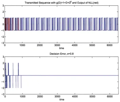
3-7 Exact form LLR NLL with input a = 0.8. The top plot shows the NLL

locks unto LFSR sequence after about 50 chips. The error decreases to zero in bottom plot. . . . . 50

3-8 Approximate scalar NLL with A = 0.33 input or = 0.8. The

approx-imate scalar NLL locks unto LFSR sequence at about the same time with exact form NLL. . . . . 51 3-9 The probability of synchronization for both exact form and

approxi-mate NLL with noise o = 0.4. . . . . 51 3-10 The probability of synchronization for both exact form and

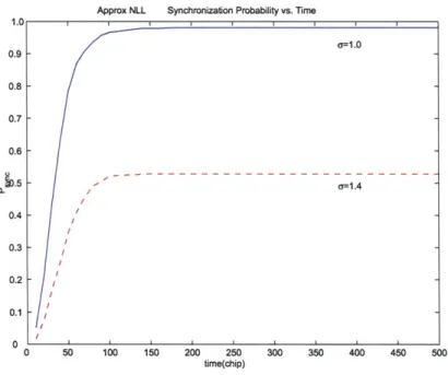
approxi-mate NLL with noise a = 0.6. . . . . 52 3-11 The probability of synchronization for approximate scalar NLL with

noise o = 1.0 and 1.4 . . . . 53 3-12 LFSR transmitter constructed with analog filters and multipliers. It

gives m-sequence with length of 15 . . . . 54

3-13 LFSR sequence generated by our analog transmitter with chip

dura-tion of 7.7ps. The lobes are notched at harmonics of the frequency 128.8KHz. The spectral lines are at harmonics of period frequency 8.59K H z. . . . . 55

3-14 Overall system simulated in CppSim. For performance comparison, approximate NLL, exact form NLL and linear filter are constructed. Two loops in the graph are approximate NLL and exact form NLL. Linear filter is implemented with the same filter in NLL to set up same comparison condition. . . . . 56 3-15 The spectrum is truncated by the filter bandwidth. This indicates our

noise calculation should only consider in-band noise. . . . . 57

3-16 The simulation result for mean square error performance for

approxi-mate scalar NLL, exact form scalar NLL, and linear filter. At very low noise(SNR> 8dB) regime, the three perform very close. At very high noise(SNR< -3dB) regime, all of them suffer big MSE. In between, the approximate scalar NLL outperforms the other two, especially when

SNR is around 5dB to 0.5dB. . . . . 58

3-17 Factor Graph of a g(D) = 1 + D + D4 LFSR sequence . . . . 59

3-18 A Cyclic factor graph for the joint conditional probability distribution p (x ,sly ). . . . . 62

4-1 Current mirror as a simple current mode translinear circuit with neg-ative feedback creating inverse function. . . . . 66

4-2 Gilbert multiplier core circuit. . . . . 68

4-3 Gilbert multiplier core circuit in a more familiar form . . . . 69

4-4 Two diodes realize inverse hyperbolic tangent function. . . . . 70

4-5 Functional block diagram of AD835. . . . . 74

4-6 LTC1064-3 8th order Bessel filter frequency response with cutoff fre-quency of 66.67kHz. From the phase plot, we can calculate the group delay to be 7.7ps, which sets the LFSR chip rate of 128.8K chips/s. The magnitude rolls off to about -13dB around 128.8KHz. This cuts off the side lobes of the spectrum of LFSR sequence. . . . . 76

4-7 Each LTC1064-3 filter connects to a post filter to further kill the clock feedthrough. The AC coupling makes the system insensitive to the filter offset. . . . . 77

4-8 Input SNR=1.4dB. The top two plots are output waveform of NLL and linear filter. The bottom two are the thresholded output of NLL and linear filter. We can see both of NLL and linear filter successfully recover the data. . . . . 79

4-9 Input SNR=-2.ldB.The top two plots are output waveform of NLL and linear filter. The bottom two are the thresholded output of NLL and linear filter. Linear filter output has been more severely disturbed by noise. The thresholded output of linear filter contains glitches which

come from the high frequency noise in the filter output. . . . . 80

4-10 Input SNR=-4.6dB. The top two plots are output waveform of NLL and linear filter. The bottom two are the thresholded output of NLL and linear filter. We zoom in to see the bit errors. By manual observation on the oscilloscope, the bit error rates of NLL and linear filter are about 10% .. . . . . . 81

4-11 Translinear block for intermediate message computation. . . . . 83

4-12 Translinear block for updated message computation. . . . . 84

4-13 Computational block for message p'(k, k - 1)oo. The blocks marked with "T1" are the tranlinear circuit in Fig.4-11, which computes the multiplication of three messages and divide by the fourth message. The blocks marked with "+" are current summation, which actu-ally are simply junctions of wires. The top four inputs are mes-sages pt-1(k - 1, k - 2)oo,o1,1o,11. The left four inputs are messages pt-1(k-2, k-3)oo,ollo,11. The bottom four inputs are messages

5-1 W inner-take-all cell. . . . . 89

5-2 Local negative feedback increases conductance . . . . 90

5-3 Block diagram of small signal analysis of WTA. . . . . 90

5-4 Feedback block diagram-1... . . . . . . . . 91

5-5 WTA in feedforward path and current mirror in feedback path. . . . . 92

5-6 N-feedback configuration . . . . 93

5-7 Ioutl of N-feedback when sweeping Iji, at different Iin2. . . .. . . .. 94

5-8 Control current gain by changing the well voltage of PMOS current-mirror. Middle point also moves. . . . . 95

5-9 P-feedback configuration... . . . . . . . . . 95

5-10 Iontl of P-feedback when sweeping fini at different 'in2.. . . . . 96

5-11 Dual feedback configuration. . . . . 96

5-12 Dual feedback. Balance point is set only by Iin2. . . . .. . . . . . . . 97

6-1 The usual geometry of the underdamped second-order transfer func-tion. Assuming di =

IP1F

IP

6-2 The new geometry proposed in [23]. Frequency point is transformed to (xo, 0). Poles are "compressed" to one Q-point. Gain is 1/d. The length L =

Vxz/Q.

6-3 The phase of the transfer function is 101i - 02, which has already been pointed out in section on usual geometry. By mirroring the two poles to right half plane, the phase can be represented by one angle. . . .. 105

6-4 When the frequency point is outside the circle, the phase written in two angles is -01 - 62. It can be also represented as one angle. . . . . 106

6-5 The key observation is that the area of triangle AP1FP2 only depends on quality factor

Q

6-6 The gain peaking happens at the point F2, where semi-circle with di-ameter P1P2 intersects with the

jw

List of Tables

Chapter 1

Introduction

A mathematical optimization problem is to minimize an objective function under a

set of constraints. Inference problem is a special kind of mathematical optimization problem with constraints including axioms of probability theory. How to construct physical systems to solve the inference problem with very low power, and/or in ex-tremely high speed, and/or with low cost, and/or with very limited physical resources etc is still a open question. Message-passing algorithms [12] [16] [5] are a special method of solving associated inference problem by locally passing messages on a fac-tor graph. The messages can be mapped into physical degrees of freedom such as voltages and currents. The local constraints on the factor graph are the computation units implemented by a class of analog statistical signal processing circuit, which we

call analogic [29].

In this thesis, we study analogic in a special test case called Noise-Locked Loop(NLL)

[28] [6]. NLL is a pseudo-random code estimation system which can perform

direct-sequence spread-spectrum acquisition and tracking functionality and promises orders-of-magnitude win over conventional digital implementation [29]. We now review the previous work on NLL.

1.1

Review of Previous Work

The history of noise-locked loop can be traced back to a nonlinear dynamic system called analog feedback shift register(AFSR) proposed in [6], which was an analog generalization of digital linear feedback shift register(LFSR). The AFSR can entrain to the pseudo-random sequence to achieve synchronization. [28] thoroughly studied different nonlinear functions to find a simpler implementation of AFSR and better performance. The most successful nonlinearity found was a quadratic function which gave very predictable mean acquisition time and can be easily implemented in elec-tronics. This is an important discovery which has interesting relation with the system we built in this thesis.

As mentioned before, analogic is a class of analog statistical signal processing circuit that propagates probabilities in a message-passing algorithm. As an exemplary em-bodiment of the new approach, an LFSR synchronization system was derived using the message-passing algorithm on a factor graph. This new system was called Noise-Locked Loop(NLL). It is very interesting to notice that NLL can be also viewed as running the noisy sequence through a soft or analog FSR [30]. This connects NLL as a statistical estimator to the AFSR as a nonlinear dynamic system. The synchro-nization performance of NLL and its comparison with maximum-likelihood estimator were also studied in [29] and [30]. The real electronic implementation was reported in [2] and [3]. In their message-passing algorithm, the messages were represented as the probabilities of binary state variables(called probability representation). In their implementation, each message represented as two probabilities was mapped into two normalized currents in current-mode circuits called "soft-gates" [18].

Belief-propagation algorithms give exact marginalized probability when the associ-ated factor graph has tree structure. However, when the factor graph involves loops, they can only compute approximate marginalized probabilities. The work in [31] [32]

[33] has pointed out that belief-propagation achieves local minima of Bethe free

en-ergy in any graph. Kikuchi free enen-ergy approximation is an improvement to Bethe free energy. By using Kikuchi free energy, a new message-passing algorithm called

Generalized Belief Propagation(GBP) was constructed. GBP is reported to be much more accurate than BP. A novel way of using GBP to improve NLL was proposed in [29] and later in [4]. Their simulation results showed better synchronization per-formance of improved NLL. But we haven't seen any physical implementation of GBP.

1.2

Motivation

Much work has been done on NLL. But there are more interesting questions that motivate of this thesis.

Firstly, most of the previous work including simulation and implementation of NLL has been focused on studying the probability representation. In this representation, message is probability. And probability is mapped into currents in the current-mode analogic circuits. So each message on the graph needs two wires to carry two cur-rents, which are complementary to each other and they must be normalized to a fixed tail current Itail in each soft-gate. Also each message needs a pair of current-mirrors to interface with soft-gates. It is natural to ask whether we can use other message representation so that messages can be mapped into voltages. In this way we may be able to save the power overhead on current-mirrors.

Secondly, most of the previous work including derivation of NLL from passing algorithms and implementation has also focused on the exact form message-passing computation, by which we mean the computation is exactly derived from message-passing algorithms. The voltage mode soft-gates has been used in analog de-coders [10]. However the voltage representation unavoidably suffers from temperature variation in the system. It is interesting to ask whether we can do message-passing with some approximate computation, what kind of approximation we can use, and if we can overcome the problem described above. This question motivates our explo-ration on approximate scalar NLL.

Thirdly, since the NLL is derived for pseudo-random code estimation, the previous work has naturally focused on its pseudo-random code synchronization performance and comparison with existing LFSR synchronization scheme in spread-spectrum sys-tems. Actually in the front end of any direct-sequence spread-spectrum system, even before signal reaches the synchronization device, there is usually some low pass filter that serves to kill the wide-band noise and clean the signal. Higher noise rejection in this filter will greatly improve the later circuit performance. NLL models both the channel noise as additive white Gaussian noise and the dynamics of LFSR. We may ask if we can use NLL to replace the linear filter that NLL gives better noise rejection.

Fourthly, the messages passed on "conventional" NLL are probabilities of one state variable. We call this NLL scalar NLL in the following chapters. The improved NLL with GBP passes messages that are probabilities of a pair of state variables. We call this improved NLL vector NLL. How to implement vector NLL using analogic is a very interesting problem, because the analogic circuits used in vector NLL may also be used in other GBP systems.

Last but not least, the previous research and motivation in this thesis both point to the direction of improving scalar NLL to vector NLL. The circuit structure are inevitably becoming more complex in vector NLL. How to build large analog network is a question that we must ask in next step. This motives another part of the work in this thesis, which is analog signal restoration.

1.3

Contribution

Here we summarize our main results in the thesis.

1. We studied scalar NLL in the approximate log-likelihood ratio(LLR)

require normalization in each soft-gate. We compared its synchronization per-formance with the NLL using exact log-likelihood ratio representation in simu-lation. The result shows approximate NLL outperforms the exact one in terms of acquisition time at low SNR regime. We implemented the approximate scalar

NLL in discrete electronics. The measurement results confirmed the simulation.

The approximate soft-gate allows us to freely set the scaling factor for conver-sion from LLR to voltage. In this way, the voltage representation is independent of temperature. This solves the problem in the exact form LLR soft-gates. We started to apply this approximate message-passing algorithm to bigger analog network such as iterative analog decoder. The preliminary results indicate the approximate algorithm work well. The temperature independent property of the voltage representation in the approximate algorithm can be very desirable for large analog network.

2. We investigated the possibility of replacing linear filter in the front end of spread-spectrum system with approximate scalar NLL. Both simulation and experiment suggest that NLL can improve the noise rejection performance in terms of mean squared estimation error. However the improvement is not very significant.

3. We proposed a translinear circuit structure for GBP, which to our best

knowl-edge is the first circuit implementation of GBP. In our circuit, messages are represented as current. The proposed circuit accomplished current production and quotient which can be used as the basic circuit primitive in general GBP systems.

4. We proposed a novel current-mode feedback amplifier with controllable gain, wide linear range, and saturation at both zero current and tail current. The basic structure is winner-take-all(WTA) cell as a high gain current amplifier in the feedforward path and current mirrors on the feedback path. The amplifier can be used in analog signal restoration.

5. We proposed a new geometric approach for all-pole underdamped second-order

transfer functions, which will be useful in the design and analysis of filters in

NLL.

1.4

Thesis Outline

In chapter 2, we introduce the necessary background information and related top-ics, including phase-locked loop, spread spectrum system, and message-passing algo-rithm. The title is termed as "from PLL to NLL", since the NLL can be viewed as a generalization of PLL from periodic signal synchronization to nonperiodic signal synchronization.

Chapter 3 derives in detail the different kinds of NLL from message-passing algo-rithm. From the simplest scalar NLL to first order Markov structured vector NLL to full trellis processing vector NLL, the performance improves, while algorithm is also more and more complex. For the scalar NLL, we proposed an approximate NLL, which is even simpler than the exact form NLL. We also started to study the appli-cation of approximate message-passing in a bigger analogic network.

Chapter 4 is on the circuit implementation of scalar NLL and circuit proposal for vector NLL. We will describe the system design of the scalar NLL with detailed dis-cussion on each components.

Chapter 5 is on current-mode signal restoration which is a very important topic for building big robust analog circuits. We propose a novel current-mode feedback am-plifier.

Chapter 6 is a diversion on second-order filter theory. We include it in this thesis because it provides useful geometric techniques for the design and analysis of filters in NLL.

Chapter 7 is summary of the work in the thesis and discussion of future research direction.

Chapter 2

Background Information

In this chapter, we try to ask some basic questions that relate to the background of the thesis. These questions include: what signal does noise-locked loop synchronize to? What is the synchronization usually implemented? What knowledge do we need

in order to understand NLL?

The simple answer to the first question is that NLL locks unto certain noise-like signal. This signal pattern is called pseudo-random signal or LFSR sequence or m-sequence, which is one of the basic spreading codes used in spread spectrum systems. More detailed review is given in first section. The second question requires us to briefly review the basic synchronization and tracking techniques used in spread spectrum systems. The third question touches the theme of the thesis which is formulating LFSR synchronization problem as a code estimation problem on the factor graph and use message-passing algorithm to obtain optimal or suboptimal solution. So in the third section we introduce the message-passing algorithm.

Before we answer all these questions, we introduce the phase-locked loop which is well known to be able to lock unto a periodic signal. After we understand PLL, it will be easier for us to understand pseudo-random code synchronization in spread-spectrum system.

2.1

Phase-Locked Loop

The PLL structure was first described by H. de Bellescize in a French journal L'Onde Electrique [14] in 1932. The background was that British engineers developed an alternative to the super heterodyne AM receiver, which was called homodyne or syn-chrodyne system. PLL was used in the homodyne receiver to automatically keep the phase of local oscillator locked unto that of the incoming carrier. In this way, the demodulation produces the maximum output. After that, the PLL was used in standard broadcast television, stereo FM radio, satellite communication systems. However, phase-locked systems were too complex and costly for use in most consumer applications. In 1970's integrated circuit process technology advanced enough to be able to fabricate monolithic PLL's at very low cost. Since then the Phase-locked loop has become universal in modern communication systems. It has been used in frequency synthesis, frequency modulation and demodulation, and clock data recov-ery(CDR),etc [14] [27].

The basic PLL is composed of phase detector, loop filter, and voltage-controlled os-cillator(VCO). The PLL pull-in process is highly nonlinear in nature. After PLL acquires locking, we can assume linear mode operation of the loop, where VCO has the linear relationship between its output frequency F0ost(t) and input control voltage

v(t) as

Fout(t) = Kvv(t). (2.1)

The output phase can be written as integration of frequency:

(bout

(t)

=

J

2,7rKv(r)dr.

(2.2)

K

<boIt(S) = -"v(s). _(2.3)

The phase detector compares the phase of the sine or square wave generated by VCO with the phase of the reference signal and produces the phase difference. For the sine wave reference signal as

linear range

Figure 2-1: Phase detector characteristics.

The VCO output is represented as

out(t) = - A, sin(wot

+

If the phase detector is an ideal multiplier followed by a low pass filter to remove the

double-frequency component, the phase detector output is

e(@) = Kd sin(@). (2.6)

where = - 0 0 and Kd is a constant. In linear mode operation, |@'I< 1, the phase detector characteristics shown in Fig.2-1 is linear to a good approximation. The loop filter exacts the average of the phase difference. When the VCO generated signal locks onto the reference signal, the phase difference is confined within small range. In this small range, the phase detector looks like a linear gain element. When the reference signal phase starts to shift away from the VCO output phase, the loop filter feeds an averaged non-zero phase difference as the control voltage to VCO. If the reference signal phase leads the VCO phase, control voltage increases to drive VCO produce higher frequency output to catch up. If VCO leads, control voltage decreases to produce lower frequency output in order to wait for reference signal. In this way, when the phase of these two signals are locked, their frequencies also become identical. The block diagram of the basic PLL structure with its linear model is shown in the Fig.2-2.

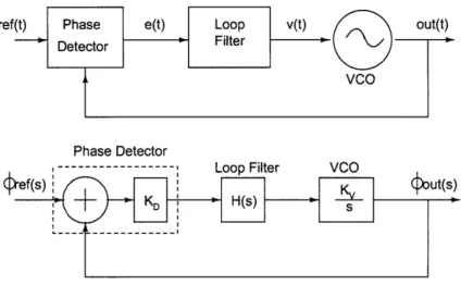
ref(t)

Phase Detector

Figure 2-2: Basic PLL structure composed of phase detector, loop filter, and voltage-controlled oscillator. Once acquisition is achieved, the PLL is modelled as a linear feedback system.

2.2

Spread Spectrum Systems

In this section, we briefly review the spread spectrum(SS) system with emphasizing on pseudorandom sequence generation and code synchronization techniques.

Pseudorandom Sequences

The general circuits that are used to generate linear feedback shift-register codes are shift registers with feedback and/or feedforward connections. Consider the logic circuit illustrated in Fig.2-3. The boxes with letter 'D' represent unit delay ele-ments,implemented as shift registers. Circles containing a "+" sign is a modulo-2 adder also called XOR gates. The coefficients besides the lines pointing to the XOR gates are either 1 if there is connection or 0 if no connection. The generating poly-nomial is defined as:

g(D) = go + giD + ... + gm-iDm- + gmDm (2.7)

Notice this generator might generate many different sequences starting from different initial states. The longest possible sequence has the period of 2' - 1, which is called

systems. Other spreading code can be derived from maximal-length sequence. Two

Figure 2-3: Linear feedback shift-register generator.

conditions must be satisfied to achieving the maximal-length sequence: the generating polynomial is primitive and the LFSR registers are initialized in non-zero state. The power spectrum of m-sequence with chip duration T, and period T = NTc has the

form

00

Sc(f) = E PnJ(f - nfo) (2.8)

2%=-oo

where Pn = [(N+1)/N2_]sinc2_{(n/N) and fo = 1/NTc. So the power spectrum consists}

of discrete spectral lines at all harmonics of 1/NTc. The envelope of the amplitude of these spectral lines is a sinc function, except the DC value is 1/N 2_{. In most}

spread-spectrum systems the power spread-spectrum of modulated data is continuous, because the carrier is randomly modulated by data and spread code.

In our further study of NLL, we take a simple case of the m-sequence generated by LFSR with polynomial g(D) = 1+ D + D4. The m-sequence generator and its output

of one period are shown in Fig.2-4.

Synchronization of PN Sequence

The spread spectrum receiver despreads the received signal with a special PN code sequence, which must be synchronized with the transmitter's spreading waveform.

D D D D

out(t)

out(t)= 1 1 1 1 0 1 0 1 1 0 0 1 0 0 0

Despreading mixer

Received signal Bandpass Energy Decision

reference signal

Reference pControl Logic

PN Generator _frequency,

Figure 2-5: Serial-search synchronization system evaluating the phase and frequency of a spreading waveform[22].

As little as one chip offset will produce insufficient signal energy for the reliable data demodulation. There are two parts of synchronization process. One is initial code acquisition. The other is code tracking. There are several ways for the initial code acquisition. One is to use correlators to correlate the received signal with local gener-ated LFSR sequence, and stepped serial-search the phase and frequency uncertainty cells until correct cell is found. The single-dwell search system always integrates over fixed interval or correlation to decide whether the acquisition is achieved or not. Multiple-dwell search system integrates over short correlation window first, if acquisition looks promising increase the window size until acquisition achieves or not. Circuit complexity is increased but acquisition time is reduced. Serial search is by far the most commonly used spread-spectrum synchronization technique. Fig.2-5 is a system block diagram.

Another PN acquisition approach is to use matched filter, which is matched to a segment of the direct sequence spread waveform. In contrast to evaluating each rela-tive code phase as serial search scheme does, matched filter synchronizer freezes the phase of the reference spreading code until a particular waveform comes(identified by the matched-filter impulse response). Once the matched waveform is received, the filter produces a pulse to start the local code generator at the correct phase. In this way, the synchronization time is improved by orders of magnitude. The principal issue limiting the use of matched-filter synchronizers is the performance degradation due to the carrier frequency error and limited coherent integration time[22]. Fig.2-6

Received _{Ba pass}

Signal Bandpass Envelope Threshold

Filterat Detector Cmaao

Threshold

Spreading Code Strobeh iStart Tracking Loop

On-Time Code

On-Time _{Data to User} , Despreader ,

Data Detector

Figure 2-6: Direct-sequence spread spectrum receiver using matched-filter code acquisition [22].

is a block diagram of a direct-sequence spread spectrum receiver using match-filter synchronizer.

The third acquisition scheme is recursion aided sequential estimation(RASE) and its extensions. The m-sequence generator described in Section2.2 contains m symbols of the code sequence. If these m symbols can be estimated with sufficient accuracy, then they can be loaded into the identical shift register generator in the receiver to synchronize the system. This approach outperforms all the serial search techniques at medium to high received SNR. For very low SNR and no priori information of the received code phase, RASE has approximately the same mean acquisition time with serial search. If a priori information about received code phase is available, the serial search performs better[22]. The block diagram of RASE synchronizer is shown in Fig.2-7.

The initial code acquisition systems position the phase of the receiver generated spreading waveform within a fraction of a chip of the received spreading waveform phase. Tracking loop takes over the synchronization process at this point and pulls the receiver spreading waveform to the precise phase. The code tracking is accomplished using phase-locked loop very similar to those used for carrier tracking discussed in

Received

Figure 2-7: RASE synchronization system.

Sec.2.1. The principal difference is in the implementation of phase detector. The

carrier tracking PLL often uses simple multiplier as phase detector, whereas code tracking loops usually employ several multipliers and filters and envelope detector[22].

A typical code tracking loop called Delay-Locked Loop(DLL) is shown in Fig.2-8,

where the PN sequence is correlated with advanced and delayed signals which goes through loop filter to VCO that drives the speading waveform generator. A similar system to DLL is Tau Dither Loop(DTL), which alternate between doing correlation with advanced or retarded signal. The output of the correlator goes to the filter which is envelope detected. If it came from retarded signal, it will be inverted before it goes into VCO. The advantage of DTL is that there is no need to match two loop filters and correlators perfectly.

2.3

Message-Passing Algorithms

In this section, we introduce message-passing algorithms, which are a key tool used in deriving scalar NLL and vector NLL in the following chapters. Message-passing algo-rithms marginalize given joint probability distribution P(u, s, x, y) to certain marginal conditional probability distribution such as P(uly).

An example is channel coding, where a vector of information bits u is mapped to a vector of codeword signals x by adding in redundancy. The encoder state is rep-resented as variable s. After signal x is transmitted across the noisy channel, the

Delay-lock Phase

Figure 2-8: Conceptual block diagram of a baseband delay-lock tracking loop.

receiver receives a noise-corrupted version y and makes estimation on the informa-tion as u.

From a probabilistic point of view, we can first specify a probability distribution for the information symbols as P(u). The encoder state is determined from the informa-tion symbols using distribuinforma-tion P(slu). The codeword is generated according to the internal state of encoder and information symbols by P(xIs, u). Finally the received signal y is related to the transmitted codeword by P(ylx). The joint probability distribution is factored as:

P(u, s, x, y) = P(u)P(slu)P(Xlu, s)P(yIX).

The significant point here is the joint probability distribution over information symbol

u, encoder state s, transmitted codeword x, and received signal y has been

decom-posed into a factorization form according to the probabilistic structure of the model.

By taking advantages of such structure, algorithms more efficient than brute-force

Bayes' rule can be designed.

The probabilistic structure can be intuitively presented on graphs. Several kinds of graphical model have been extensively researched, such as Bayesian network, Markov random field, and factor graph[19] [13] [16].

For our channel coding example, the factorized join probability distribution can be drawn in Bayesian network as:

Figure 2-9: Bayesian Network for Channel Coding

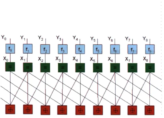
In the following we will use a normal factor graph, because factor graph gives an easier way to show the constraint relations between variables. It also provides a straightforward way to present the process of marginalization, which is known as message-passing algorithm. The essence of message-passing on a tree is illustrated in Fig.2-10. The boxes represent the functions or constraints. The edges represent the variables. For example, box fi connected with edge x1 means the fi is the function of

variable x1. The messages are passed between boxes and edges. For example, message

pf4-.24 is passed from function node

f4

X

marginalized probability distribution. The calculation of the marginal probability for certain variable from the global joint probability distribution of all the variables is obtained by successive local message-passing. The example shown in Fig.2-10 is on calculating marginal probability p(x4). The process is as following.

First, obtain message pf31X4 as

pf3_.24 = E E

E

f3(,

X1 X2 X3

Second, obtain message pf6_2,, as

prf-+X6 =

fX(

X7 X8

Third, we can get message ph'X4 from message tf_{6 -X6} as

Pf4-24 = ZE

f4(x4,

X5 X6

Finally the two messages passing from opposite directions are combined to get the marginal probability p(X4) as

Iff xx xx fX2 x f4 8 x3 R12

Figure 2-10: Message-passing process illustrated on the tree-like factor graph. Mes-sage p1 in the figure represents mesMes-sage pf3 , in the above derivation. Message pL2

represents If 4-*X4. p13 represents pr-+X6

[121.

The general sum-product algorithm operates according to this simple rule[12]:

Sum-Product Update Rule:

The message sent from a node v on an edge e is the product of the local function at v(or the unit function if is a variable node) with all messages received at v on edges

Chapter 3

LFSR Synchronization: From

Scalar NLL to Vector NLL

In the previous chapter, we reviewed the basic phase-lock technique, basic concepts of spread spectrum, and message-passing algorithms. These provide the background knowledge for this chapter.

As reviewed in Chapter 1, the previous work in [29] and [4] studied scalar NLL and proposed vector NLL. In this chapter, as a good exercise to solidify the ability of com-munication in the language of message-passing algorithms, we rework out by ourselves the math of scalar NLL and vector NLLs. We connect them together by emphasiz-ing performance improvement from simple suboptimal estimation(scalar NLL) usemphasiz-ing belief-propagation algorithm to intermediate complexity estimator (vector NLL) us-ing generalized belief-propagation.

The previous work has been mainly focused on exact form message-passing algo-rithm. By "exact form message-passing", we mean that the basic computations of messages use their exact mathematical form. For example, the parity-check node in log-likelihood ratio representation involves hyperbolic and inverse hyperbolic func-tions(see Section.??). An interesting question to ask is how robust the message-passing algorithm is when the basic computation is not accurate. More precisely, what is the algorithm performance if the basic computation has been changed to an

Figure 3-1: Approximate scalar NLL.

multiplier

+

Delay

X

(nonlinearity)

Figure 3-2: Continuous state, continuous time, AFSR[28].

approximate form. The reason to ask this question mainly comes from the considera-tions on practical implementation of message-passing algorithm in physical systems, especially large-scale systems. But we do not tend to maintain the exact form com-putation by merely battling with the nonidealities in the circuit through some circuit techniques, which has been studied in [18]. Rather we consider the problem at a higher algorithmic level. We intend to construct some mathematically approximate computation to replace the exact computation in message-passing algorithms. This makes it possible to construct temperature independent or very weakly temperature dependent analogic circuit in a principled way.

It is interesting to point out that the approximate scalar NLL in Fig.3-1 has a similar structure with AFSR in Fig.3-2, which was proposed at the end of Ben-jamin Vigoda's master thesis [28]. Vigoda originally came up with this configuration in Fig.3-2 from the perspective of nonlinear dynamic system. And he discovered

it mainly by numerical experimenting. Here we study the approximate scalar NLL as a suboptimal estimator derived from message-passing algorithms. The simulation shows the approximate scalar NLL has better synchronization performance than exact form scalar NLL. It is hard to explain by message-passing algorithms. The nonlinear dynamics approach taken in Vigoda's master thesis might provide some hints on the explanation.

Both vector NLL and scalar NLL are non-iterative estimation. We proposed an iter-ative LFSR synchronization algorithm at the end of this chapter. Then we compare scalar and vector NLL in terms of computational complexity and synchronization performance.

3.1

LFSR Synchronization as Maximum Likelihood

Estimation

Consider a sequence of symbols x={xk} generated as an m-sequence and transmitted over an additive white Gaussian noise channel(AWGN) with output

Yk = Xk + Wk. (3.1)

We are interested in the a posteriori joint probability mass function for x={xk} given the fixed observation y={yk}:

(x) = p(xjy) oc p(x)f(yjx), (3.2)

where f(ylx) is the priori probability distribution. If the a priori distribution p(x) for the transmitted vectors is uniform, then

4'(x) oc f(y x). (3.3)

The marginal conditional distribution has the form

which marginalizes for each xk by summing over all variables except Xk. The receiver selects the value of Xk that maximizes each marginal function in order to minimize the probability of error over each symbol. The acquisition of m-sequence is, therefore, through maximum-likelihood(ML) or maximum a posteriori(MAP) detection. The a posteriori probability distribution can be represented by a cycle-free trellis through a hidden Markov model. At any given time k, define state variable Sk, the output from transmitter Xk, and the channel observation Yk. The Markov model is hidden because Sk is not observable; only noisy version yA is observable.

p(x,sly) oc p(x,s)f(ylx,s), (3.5) = p(x)p(slx)f(ylx), (3.6) c p(sjx)f(yjx), (3.7) N-1 = I(x,s,y) 11 f(yklxk), (3.8) k=0 N-1 N-1 =

II

where assume the a priori distribution p(x) is uniform, N is the length of observation, and Ik(Sk, Xk, Sk+1) is the indication function that constrains the valid configuration of each individual state and transmitted symbol. The normal factor graph for this trellis is in Fig.3-4.

x, jx

jx2

fo f f2 f3|

YO

V1

Y31

Figure 3-3: A Cycle-free normal factor graph for the joint conditional probability distribution p(x,sly).

For each transmitted symbol Xk, the detection gives the a posteriori probability as

/k(Xk) - p(XkIy) c p(x,sly). (3.10)

Next we explicitly write down the messages and the message-passing procedure.

1. Message initialization:

(a) messages from y to fA: pYk-5k - 6(yk, Yk).

(b) message at the beginning of observation: ps 0-Io = 1.

(c) message at the end of observation: p3NN 1.

2. Forward message passing through sk:

IIk-1Sk =

S S

Sk-1 Xk-1

3. Backward message passing through sk:

1

1k-Sk =

S

X(,sk+1)1k2xk)Ik.1-Sk.1-Sk+1 Xk

4. Messages passing through xk:

pXk -Ik = 53(yk, y)f(xkIyk) = f(xklyI), (3.13)

Yk

Ik-xk Ik-1*Sk0Ik+1 Sk+1'

(3.14)

Sk Sk+1

5. A posteriori probability of Xk:

P(kY= Pxk'Ik ' MIk-+xk. (3.15)

If we are only interested in the ML detection of current state rather than ML detec-tion of the old states by updating the whole history, which is the case for our code acquisition, then the a posteriori probability of current symbol XN+1 can be easily

calculated by the knowledge of formal state P(XNjy). Forward-backward message-passing is simplified to "forward-only" message-passing. Note that "forward-only" here means we don't need to calculate the backward messages Alk -Sk. Calculation of P(XN+1 y) must always do P(XN+1Iy = IxN+1-IN+1 [LIN+ ₁-XN+l, which is still locally

3.2

Exact Form Scalar NLL

The trellis processing guarantees the maximum likelihood detection. However, the computation complexity is exponential with r the number of LFSR stages, because the branches at each trellis section is 2' - 1. It is desirable to find low-complexity

suboptimal algorithm. The hint comes from the fact that there are usually several factor graphs representing one probabilistic structure. For our m-sequence acquisi-tion problem, an alternative factor graph is constructed by considering the generating polynomial of m-sequence. Because there is no need for receiver to update the esti-mation of all history at each time step, the forward-only message passing is used to achieve the current state estimation. This low-complexity estimator with forward-only message-passing algorithms is called scalar NLL.

o

Y,

Y

2

Y

4

Y'

Y

Y

Ye

Figure 3-4: A cycle normal factor graph for the joint conditional probability distri-bution p(xsly).

There are several representations of messages in NLL. Each results different com-putations [30]. Now we derive the two representations: probability representation and log-likelihood ratio representation. These two are closely related to the devel-opment of scalar NLL in following sections. The message computations of soft-Xor and soft-equal in these two representation derived below both use the exact form computation.

3.2.1

Probability Representation

The previous work on scalar NLL has been focused on this representation. Both simulation and implementation [2] [3] has been published. y(t) is the observation of the channel. x(t) is transmitted signal. f(y(t) Ix) is the priori probability distribution

of two. 1. Mathematical derivation: Conversion block: 1 f (y(t)jx = 1) = exp(-(y(t) - 1)2/202), (3.16)

v27ro.

p(x = 1|y(t)) = f(y(t)Iz = 1) +

f

(y(t)|z

px = -1|y(t)) = f (y(t)| 1)

f

Soft-Xor gate:

Pxor(1) = Pxi(0) -px4(0) + Pxl(1) - p4(1), (3.20)

Pxor (0) = poi (0) -A p(1) + pxli(1) -A p(0). (3.21)

Soft-equal gate:

pxor (1) -p(x = I|y(t))

peqi(1) = Pxor(l) -p(X = 1|y(t)) +Pxor(O) -p(X = -1|y(t))' (3.22)

SPxor (0) -p(x = -1|y(t))

3.2.2

Log-Likelihood Ratio(LLR) Representation

The LLR representation of NLL has been proposed in [30]. The exact form LLR soft-Xor involves hyperbolic tangent function and inverse hyperbolic tangent function as shown in Eq.3.25, which will be approximated in the approximate scalar NLL.

1. Mathematical derivation:

Conversion block:

p (t) = 2y(t) (3.24)

Soft-Xor gate:

pxor = 2 tanh-1(tanh(

)

2 2

Soft-equal gate:

1

eqI = pxor + py. (3.26)

3.3

Approximate Scalar NLL in Log-Likelihood

Ra-tio(LLR) Representation

The exact form LLR soft-Xor in Eq.(3.25) has been implemented with Gilbert cell and inverse hyperbolic function circuits stacked at output of Gilbert cell [10]. The circuit realized the following function:

V1 V2

Vot = 2VT tanh-1(tanh( ) tanh( )). (3.27)

2VT 2VT

The log-likelihood ratio was represented as V/VT. Although the circuit faithfully realized the exact mathematical functions, the thermal voltage VT = kT/q in the

scaling factor makes LLR unavoidably subject to temperature variation. This concern has also been pointed out by Lustenberger in his Ph.D. thesis [18]. The conclusion there was negative on voltage-mode log-likelihood ratio implementation. However, if we gave up the insistence on exact form soft-gates, we will have a new view. Here, we put the inverse hyperbolic function circuit in the input instead at output of Gilbert cell, to recompense the hyperbolic function in Gilbert cell, we will have a complete

four-quadrant analog multiplier as

Vout = a - (3.28)

a a

where LLR is represented by the ratio V, and a is an arbitrary voltage that we can set.

Three questions we need to answer are how good this approximation comparing with exact form, how good this approximate NLL performs comparing with exact NLL, and whether this approximation method can be extended in other message-passing circuits, especially the large analog network. The following three sections try to answer these questions.

3.3.1

Multiplier Approximation

The multiplier approximation is written here again:

2tanh 1 (tanh(x/2) tanh(y/2)) - Axy, (3.29)

where coefficient A is a free parameter that we choose to obtain better performance of NLL.

First we look at hyperbolic function tanh(x) and its inverse function tanh-1(x). The Taylor series expansions are

1 2 17

tanh(x) = x - - -+ ... for

Ix

3 15 315 2

13 15 17

tanh-1(z) =x + + o+ ± z + ... for

lxi

which tells us they can be approximate by the first term x in Taylor expansion, for at least IxI < 1. So roughly we have 2tanh-1 (tanh(x/2) tanh(y/2)) x zy/2, with

A = 0.5,

lxi

l|<

To more accurately determine the coefficient A, we cannot rely on the first or-der Taylor expansion. We need to do linear fitting of the whole compound function. Numerical calculation in Matlab gives the following values of A in Eq.(3.29) corre-sponding to {, y}

E

z=2atanh(tanh(x/2)tanh(y/2) and z=0.3489*xy

5

5 -

--1.5

-1.5 -1 -0.5 0.5 1 1.5 2

Figure 3-5: Dotted lines are function 2 tanh-(tanh(x/2) tanh(y/2)) plotted with

x E [-2, 2],y E {±2, +1.5, 1, +0.5, 0}. Solid lines are function 0.348 * xy.

z=2atanh(tanh(x/2)tanh(y/2)-0.3489*xy

Figure 3-6: 2tanh-1(tanh(x/2) tanh(y/2)) - 0.348 * xy, plotted for x E [-2, 2],y E

{+2, 1.5, i1, +0.5, 0}.

5 -1. -21