Depth classification of underwater targets based
on complex acoustic intensity of normal modes
The MIT Faculty has made this article openly available.
Please share
how this access benefits you. Your story matters.
Citation
Yang, Guang et al. “Depth Classification of Underwater Targets
Based on Complex Acoustic Intensity of Normal Modes.” Journal of
Ocean University of China 15.2 (2016): 241–246.
As Published
http://dx.doi.org/10.1007/s11802-016-2674-9
Publisher
Science Press
Version
Author's final manuscript
Citable link
http://hdl.handle.net/1721.1/104957
Terms of Use
Article is made available in accordance with the publisher's
policy and may be subject to US copyright law. Please refer to the
publisher's site for terms of use.
DOI 10.1007/s11802-016-2674-9 ISSN 1672-5182, 2016 15 (2): 241-246
http://www.ouc.edu.cn/xbywb/ E-mail:xbywb@ouc.edu.cn
Depth Classification of Underwater Targets Based on
Complex Acoustic Intensity of Normal Modes
YANG Guang
1), YIN Jingwei
1), *, YU Yun
2), and SHI Zhenhua
3)1) Acoustic Science and Technology Laboratory, College of Underwater Acoustic Engineering,
Harbin Engineering University, Harbin 150001, P. R. China
2) Naval Academy of Armament, Beijing 100161, P. R. China
3) Department of Mechanical Engineering, Massachusetts Institute of Technology, Boston Mit 77, USA (Received May 19, 2014; revised October 17, 2014; accepted November 30, 2015)
© Ocean University of China, Science Press and Springer-Verlag Berlin Heidelberg 2016
Abstract In order to solve the problem of depth classification of the underwater target in a very low frequency acoustic field, the
active component of cross spectra of particle pressure and horizontal velocity (ACCSPPHV) is adopted to distinguish the surface vessel and the underwater target. According to the effective depth of a Pekeris waveguide, the placing depth forecasting equations of passive vertical double vector hydrophones are proposed. Numerical examples show that when the sum of depths of two hydro-phones is the effective depth, the sign distribution of ACCSPPHV has nothing to do with horizontal distance; in addition, the sum of the first critical surface and the second critical surface is equal to the effective depth. By setting the first critical surface less than the difference between the effective water depth and the actual water depth, that is, the second critical surface is greater than the actual depth, the three positive and negative regions of the whole ocean volume are equivalent to two positive and negative regions and therefore the depth classification of the underwater target is obtained. Besides, when the 20m water depth is taken as the first critical surface in the simulation of underwater targets (40Hz, 50Hz, and 60Hz respectively), the effectiveness of the algorithm and the cor-rectness of relevant conclusions are verified, and the analysis of the corresponding forecasting performance is conducted.
Key words the placing depth forecasting equations; the effective depth; depth classification; Pekeris waveguide
1 Introduction
There are about 150 countries with coastlines around the world. At present, it is difficult to detect adversary underwater targets by conventional means, which could seriously threaten the safety of these countries. Due to the acoustic features of an underwater target in a very low frequency range (10–100Hz), this paper adopts the ACC- SPPHV to conduct the depth classification of low-noise targets, that is, the binary decision of surface targets and underwater targets, which has bright prospects of poten-tial applications in a coast warning system, such as Ver-tical Double Towed Lines Array, AeronauVer-tical Underwa-ter Acoustic Buoy, etc.
Many algorithms have been used to detect and localize underwater targets. Josso et al. (2010) investigated un-derwater targets’ motion detection and estimation. Bag-genstoss (2011) carried out localization research of mul-tiple interfering sperm whales using time difference. Dosso and Wilmut (2011) researched multiple underwater targets’ localization. Michalopoulou et al. (2011) investi-gated the passive tracking algorithm based on particle * Corresponding author. E-mail: edit231@163.com
filtering. Wiggins et al. (2012) researched the underwater targets’ tracking using a multichannel autonomous acous-tic recorder. Dubreuil et al. (2013) researched underwater target’s detection taking advantage of imaging polari- metry and correlation techniques. Diamant et al. (2014) did the underwater acoustic localization research using LOS and NLOS algorithms. Gerstein and Gerstein (2014) did some research on sound localization in shallow waters. Forero (2014) investigated broadband underwater target’s localization by multitask learning.
In this paper, the Pekeris waveguide model and ACC- SPPHV of passive vertical double vector hydrophones are used to divide the whole ocean volume into two parts, which solves the depth classification problem of under-water targets. Based on our prior research (Hui et al., 2008; Yu et al., 2008, 2009), research is conducted in imple-menting the placing depth forecasting equations based on ACCSPPHV of vertical double vector hydrophones.
2 Depth Classification Theory and Placing
Forecasting Equations
An underwater target usually radiates strong line spec-tra below 100Hz, and therefore, the Pekeris Model is employed in this paper. The waveguide diagram is shown
YANG et al. / J. Ocean Univ. China (Oceanic and Coastal Sea Research) 2016 15: 241-246 242
in Fig.1.
Fig.1 Pekeris waveguide.
The particle sound pressure equation is given as (Liu, 2010), (1) 0 1 1 0 0 ( , , ) 2π sin( n ) ( , )n ( n ) n p r z z
z F z H r π 4 1 1 0 8π 1 e j sin( ) ( , )ej rn n n n n z F z r
, (1) where 0 ( , )n F z 1 1 0 2 2 1 1 1 1 1 sin( )sin( ) cos( ) tan( )sin ( )
n n n n n n n z H H H b H H ,
n represents the order of normal modes,
2 2
1n k1 n
, b 1/ 2, ki/ ( 1, 2)c ii , ρ1 and ρ2 are the densities of seawater and seafloor,
re-spectively, z0 is the depth of underwater target, z is the
placing depth of hydrophone, r is the horizontal distance between z0 and z, εn is the eigenvalue of the nth normal
mode, which is the root of the following eigenvalue equa-tion 2 2 cos sin 0 x x jb x x , (2) where 1 xH, 2(k12k22)H2.
Every normal mode corresponds to one cut-off fre-quency fn, namely, when the frequency of a sound source
f<fn, the nth normal mode can not be motivated by the
sound source. fn can be expressed as (Liu, 2010),
1 2 2 2 2 1 1 ( ) 2 2 n n c c f H c c . (3) The relationship between particle velocity and sound pressure is (Brekhovskikh and Lysanov, 2003)
v p t
, (4) where v contains the time factor. Thus, the above equation can be written as 1 1 [ p p ] v p i k j j r z . (5) Substituting Eq. (1) into Eq. (5), the horizontal and vertical components of the particle velocity are given respectively as π 4 1 0 8π e j sin( ) ( , )ej rn r n n n n v z F z r
, (6) and π 4 1 1 0 8π 1 e j cos( ) ( , )ej rn z n n n n n v j z F z r
. (7) According to Eq. (1) and Eq. (6), the cross spectra of particle sound pressure and horizontal velocity of vertical double vector hydrophones can be obtained from its ac-tive component part as* r r I pv [( - ) ] 2 1 1 1 1 2 0 1 1 1 2 0 0 , 8π
sin( )sin( ) ( , ) m sin( )sin( ) ( , ) ( , )ej n m r
n n n n m n m n n n n m m z z F z z z F z F z r
, (8)and the vital ACCSPPHV can be obtained as = rA I 2 1 1 1 1 2 0 1 1 1 2 0 0 , 8π
sin( )sin( ) ( , ) msin( )sin( ) ( , ) ( , ) cos[( ) ]
n n n n m n m n m n n n n m m z z F z z z F z F z r r
. (9)When there are only two normal modes in underwater acoustic field, that is, only the first two normal modes are
considered in this paper, Eq. (9) can be expanded and simplified for analytical convenience:
2 2
11 1 11 2 0 1 12 1 12 2 0 2
sin( )sin( ) ( , ) sin( )sin( ) ( , )
rA
11 1 12 2 0 1 0 2 1 2 12 1 11 2 0 2 0 1 2 1
sin( z)sin( z F z) ( , ) ( , ) cos[( F z ) ] sin(r z)sin( z F z) ( , ) ( , ) cos[( F z ) ]r . (10) According to Eq. (10), when receiver points z1 and z2
are fixed and the sign of ACCSPPHV is kept unchanged with distance r, it is easy to get
11 1 12 2 0 1 0 2 1 2
sin( z)sin( z F z) ( , ) ( , ) cos[( F z ) ]r
12 1 11 2 0 2 0 1 2 1
sin( z )sin( z F z) ( , ) ( , ) cos[( F z ) ] 0r . (11) The Pekeris model can be equivalent to the environ-ment where the effective water depth is absolutely soft, and the expression of the effective water depth is (Buchingham and Giddens, 2006)
1 1 1 sin( ) e c H H bk H , (12) where He is the effective water depth, H represents the
actual water depth, b is the density ratio of seawater to
seafloor, k1 is the wave number in seawater, and αc=
cos−1(c
1/c2), representing the critical grazing angle. Then,
Eq. (11) can be converted to
1 2 1 2
π 2π 2π π sin( )sin( ) sin( )sin( ) 0
e e e e
z z z z
H H H H . (13)
Because πz1/He, πz2/He[0, π) in Eq. (13), a critical
conclusion can be drawn
1 2 e
z z H . (14) Therefore, only if the summation of the placing depths of two hydrophones equals the effective water depth, the cross spectra sign of the particle sound pressure and the horizontal velocities of the hydrophones are irrelevant to the horizontal distance r. Thus, the depth classification of the underwater target can be made based on this law. When Eq. (14) is met, Eq. (10) can be changed to
2 2
1 2 0 1 2 0
π π π 2π 2π 2π sin( )sin( )sin ( ) sin( )sin( )sin ( )
rA e e e e e e I z z z z z z H H H H H H 2 2 2 1 2 0 1 0 π π π π π sin( )sin( )sin ( ) [1 16 cos ( ) cos ( )]
e e e e e z z z z z H H H H H . (15) Assuming 2 2 1 0 [1 16cos (π / e) cos (π / e)] F z H z H ,
the sign of IrA is decided by F. Due to πz0/He[0, π),
cos2(πz
0/He) is a monotonic decreasing function when z0
[0, He/2] and a monotone increasing function when z0
[He/2, He], i.e., the function is symmetric with respect to
He/2. For a nonzero F, we can get
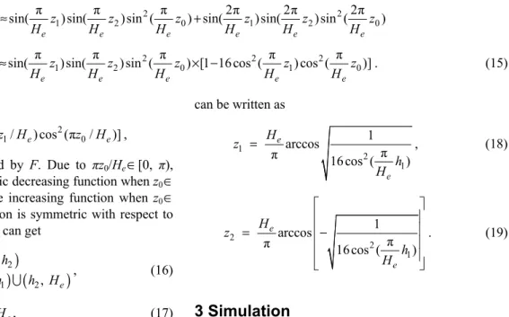
0 1 2 0 1 2 0, , 0, 0, , e F z h h F z h h H , (16) 1 2 e h h H , (17) where h1 represents 2 1 1 arccos π π 16 cos ( z ) e e H H , and h2 represents 2 1 1 arccos π π 16cos ( z ) e e H H .From Eq. (16), the whole ocean volume can be divided into three parts, negative value–positive value–negative value, within the effective water depth He, and the
sum-mation of the two critical surfaces is He. When the first
critical surface h1 is less than He−H, the second critical
surface h2 is greater than the actual water depth H. At this
time, the second negative value region is invalid. By set-ting the first critical surface h1, the theoretical forecasting
equations on the placing depth of the two hydrophones
can be written as 1 2 1 1 arccos π π 16 cos ( ) e e H z h H , (18) 2 2 1 1 arccos π π 16cos ( ) e e H z h H . (19)
3 Simulation
For single-frequency acoustic waves from a point sound source, the water depth H=100m, the particle ve-locity c1=1500ms−1, the seabed medium sound velocity
c2=1570ms−1, ρ1=1.025gcm−3, and ρ2=1.766gcm−3.
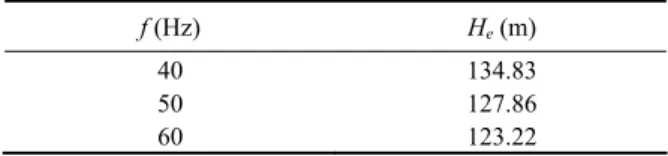
Ac-cording to Eq. (3), the cut-off frequencies of the first five normal modes are shown in Table 1. On the basis of Eq. (12), He can be obtained as shown in Table 2. When the
sound source frequency 38.1008<f<63.5013, only the first two normal modes need to be considered.
Table 1 The cut-off frequencies of the first five normal modes n fn (Hz) 1 12.70 2 38.10 3 63.50 4 88.90 5 114.30
YANG et al. / J. Ocean Univ. China (Oceanic and Coastal Sea Research) 2016 15: 241-246 244
Table 2 Effective water depths of 40Hz, 50Hz, and 60Hz
f (Hz) He (m)
40 134.83 50 127.86 60 123.22
Take 40Hz, 50Hz, and 60Hz as examples, white repre-sents the positive value, and blue reprerepre-sents the negative value.
1) The frequency of the underwater target is 40Hz. If
setting h1=20m as the first critical surface, z1=55.24m
and z2=79.59m can be obtained according to Eqs. (18)–
(19). The vertical double hydrophones are placed at the depth of z1=50.7m and z2=80.1m respectively, and Fig.
2(a) shows the results by Eq. (9). Furthermore, the sum-mation of placing depths is 130.8m. If putting the vertical double hydrophones at z1=43m, z2=88m, the summation
is 131m and the results are shown in Fig.2(b). The critical surfaces are h1=38m, h2=93m, the summation of which is
131m. All the three summations are close to the theoreti-cal effective water depth 134.83m.
Fig.2 The sign change of ACCSPPHV with f=40Hz. 2) The target frequency is 50Hz. Based on Eqs. (18)–
(19), setting h1=20m as the first critical surface, z1=52.23
m and z2=75.63m can be obtained. If the vertical double
hydrophones are placed at z1=50.9m, z2=73.1m,
respec-tively, the summation of placing depths is 124m. Fig.3(a) shows the results obtained by Eq. (9) and Fig.3(b) by
placing the vertical double hydrophones at z1=37.9m,
z2=86.3m with the placing depth summation of 124.2m.
When the critical surfaces are h1=44m and h2=80 m, the
summation of h1 and h2 is 124m. All the three
summa-tions well match the corresponding theoretical effective water depth of 127.86m.
Fig.3 The sign change of ACCSPPHV with f=50Hz. 3) The target frequency is 60Hz. On the basis of Eqs.
(18)–(19), setting h1=20m as the first critical surface, z1=
50.21m and z2=73.00m can be obtained. If the vertical
double hydrophones are placed at z1=49.3m and z2=70.9
m, respectively, the summation of placing depths is 120.2 m. Fig.4(a) shows the results by Eq. (9) and Fig.4(b) by placing the vertical double hydrophones at z1=30m and
With the critical surfaces of h1=46m and h2=74m, the
summation of h1 and h2 is 120m. All the three
summa-tions well match the corresponding theoretical effective water depth of 123.22m.
Fig.4 The sign change of ACCSPPHV with f=60Hz. According to the above simulations at 40Hz, 50Hz,
and 60Hz, the effectiveness of this algorithm is proved, and some relevant conclusions can be drawn. Placing depths of the vertical double vector hydrophones can be predicted through Eqs. (18)–(19). There are errors be-tween the predicted and actual placing positions, but they become smaller with the increase of the target frequency. The summation of the placing depths of hydrophones and that of the first and the second critical surfaces approxi-mately equal the corresponding effective water depth, which verifies Eqs. (14) and (17).
4 Forecasting Performance Analysis
Taking the same sea environment as above, the placing position comparisons of prediction and simulation with
the target frequencies of 40Hz, 50Hz, and 60Hz are shown in Fig.5. In the figure the horizontal axis is the first critical surface from 10m to 40m with an interval of 5m, and the vertical axis represents the placing depth of hy- drophones. The results show that the forecasting per- formance is improved with the increase of the sound source frequency.
The summation deviations comparisons of simulation placing and placing prediction with varying frequencies of sound sources are shown in Fig.6.
From Fig.6, a conclusion can be drawn that with the increase of sound source frequencies, the summation viations of simulation placing and placing prediction de-creases. Moreover, with the increase of the critical sur-face h1, the summation deviations show a decreasing
trend.
YANG et al. / J. Ocean Univ. China (Oceanic and Coastal Sea Research) 2016 15: 241-246 246
Fig.6 The summation deviations comparisons of simula-tion placing and placing predicsimula-tion.
5 Conclusions
Based on ACCSPPHV of vertical double vector hydro-phones, the depth classification algorithm of underwater targets is proposed to distinguish a surface vessel and an underwater target in this paper. Forecasting equations for placing depths are obtained when the summation of the two critical surfaces and that of placing depths equal ef-fective water depth. The simulation and forecasting per-formance analysis are carried out, which verifies the ef-fectiveness and correctness of this algorithm. In addition, this algorithm is simple and easy to implement, and has the potential for future applications in vertical arrays.
Acknowledgements
This study was supported by Public Science and Tech-nology Research Funds Projects of Ocean (201405036-4), the National Natural Science Foundation of China (Grant Nos. 11404406, 51179034, 41072176 and 11204109), Defense Technology Research (JSJC2013604C012), and Postdoctoral Science Foundation of China (Grant No. 2013M531015).
References
Baggenstoss, P. M., 2011. An algorithm for the localization of
multiple interfering sperm whales using multi-sensor time difference of arrival. Journal of Acoustical Society of America,
130 (1): 102-112.
Brekhovskikh, L. M., and Lysanov, Y. P., 2003. Fundamentals of
Ocean Acoustics. Third edition. AIP Press, America, 51.
Buchingham, M. J., and Giddens, E. M., 2006. On the acoustic field in a Pekeris waveguide with attenuation in the bottom half-space. Journal of Acoustical Society of America, 119 (1): 123-142.
Dubreuil, M., Delrot, P., and Leonard, I., 2013. Exploring underwater target detection by imaging polarimetry and correlation techniques. Applied Optics, 52 (5): 997-1005. Diamant, R., Tan, H. P., and Lampe, L., 2014. LOS and NLOS
classification for underwater acoustic localization. IEEE
Transactions on Mobile Computing, 13 (2): 311-323.
Dosso, S. E., and Wilmut, M. J., 2011. Bayesian multiple-source localization in an uncertain ocean environment. Journal of
Acoustical Society of America, 129 (6): 3577-3589.
Forero, P. A., 2014. Broadband underwater source localization via multitask learning. IEEE Information Sciences and
Systems Conference. Princeton, New Jersey, 1-6.
Gerstein, E. R., and Gerstein, L., 2014. Manatee hearing and sound localization can help navigate noisy shallow waters and cocktail events, no Lombard’s needed. Journal of Acoustical
Society of America, 135 (4): 2172.
Hui, J. Y., Sun, G. C., and Zhao, A. B., 2008. Normal mode acoustic intensity flux in Pekeris waveguide and its cross spectra signal processing. Acta Acustica, 33 (4): 300-304 (in Chinese with English abstract).
Josso, N. F., Ioana, C., Mars, J. I., and Gervaise, C., 2010. Source motion detection, estimation, and compensation for under- water acoustics inversion by wideband ambiguity lag-Doppler filtering. Journal of Acoustical Society of America, 128 (6): 3416-3425.
Liu, B. S., 2010. Underwater Acoustic Principle. Second edition. Harbin Engineering University Press, Harbin, 75 (in Chinese). Michalopoulou, Z. H., Yardim, C., and Gerstoft, P., 2011. Particle filtering for passive fathometer tracking. JASA Express Letters, 1-7.
Wiggins, S. M., McDonald, M. A., and Hildebrand, J. A., 2012. Beaked whale and dolphin tracking using a multichannel autonomous acoustic recorder. Journal of Acoustical Society
of America, 131 (1): 156-163.
Yu, Y., Hui, J. Y., and Zhao, A. B., 2008. Complex acoustic intensity and application of normal modes in Pekeris waveguide.
Acta Physic Sinica, 57 (9): 5742-5748 (in Chinese).
Yu, Y., Hui, J. Y., and Chen, Y., 2009. Research on target depth sorting of shallow and low-frequency acoustic field. Acta
Physic Sinica, 58 (9): 6335-6343 (in Chinese).