IdEP Economic Papers
2014 / 01
Fabrizio Mazzonna, Franco Peracchi
Unhealthy retirement? Evidence of occupation
heterogeneity
∗Fabrizio Mazzonna
University of Lugano (USI) and MEA
Franco Peracchi
Tor Vergata University and EIEF February 8, 2014
Abstract
We investigate the causal effect of retirement on health and cognitive abilities by exploiting the variation between and within European countries in old age retirement rules. We show negative and significant effect of retirement on both health and cognitive abilities. We also show evidence of significant heterogeneity across occupational groups. In particular, the negative effect of retirement disappears and turn to be even positive for those working in very physically demanding jobs.
Keywords: Aging; cognitive abilities; retirement; occupation; SHARE. JEL codes: C26, I14, J14, J24, J26.
∗
Corresponding author: Fabrizio Mazzonna, Department of Economics (IdEP), University of Lugano, via G. Buffi 13, CH-6942 Lugano (fabrizio.mazzonna@usi.ch). This paper uses data from SHARE release 2. The SHARE data collection has been primarily funded by the European Commission through the 5th, 6th and 7th framework programmes. Additional funding from the U.S. National Institute on Aging as well as from various national sources is gratefully acknowledged (see www.share-project.org for a full list of funding institutions).
1
Introduction
Declining labor force participation among aging workers, continuing growth in life expectancy and declining fertility have caused a looming financial crisis in social security programs in most devel-oped economies. In order to cope with this dramatic demographic transition, many governments have implemented public policies aimed at increasing the average retirement age of the population. However, there are dissenting opinions about not only the magnitude of these effects, but also their sign (see B¨orsch-Supan 2013 for a discussion).
On the one hand, retirement may enable individuals to enjoy their leisure time and eliminate work-related stress, with positive spillovers on their mental health and well-being. Moreover, re-tirement might be beneficial for those individuals working in physically demanding and unhealthy occupations. This argument has been strongly supported by labor unions who oppose the increase in retirement age. To this end, recent literature in Economics has shown the presence of negative effects on health of working in physical demanding occupations (see Case and Deaton 2005 and Ravesteijn et al. 2013 for a review).
On the other hand, there is a view that retirement may be harmful. This may happen if a lack of purposes in the retiree’s life affects individual well-being, mental health and cognitive abilities (Rohwedder and Willis 2010). As argued in our previous study on the effect of retirement on cognition (Mazzonna and Peracchi 2012), this negative effect can actually be predicted using the theoretical framework provided by Grossman (1972). The main intuition is that retired individuals lose the market incentive to invest in cognitive repair activities, which may lead to an increase in the rate of cognitive decline after retirement. A negative effect on health can be also predicted if retirement reduces social interactions. The social capital literature (see e.g. Glass et al. 1999 and d’Hombres et al. 2010) suggests that the social networks formed at work may buffer from health shocks. To this end, B¨orsch-Supan and Schuth (2013) argue that at least one third of the decline in cognition after retirement can be attributed to the shrinkage of social networks. More generally, retirement may affect lifestyles, such as drinking and smoking habits, dietary consumption and most importantly physical activity (Zantinge et al. 2013), which in turns may affect individuals’ health. For instance, if work is the main form of physical activity for many individual, then we might expect a negative effect of retirement on health.
In this paper we present evidence of heterogeneity in the effect of retirement on health and cognition across occupations, thus showing that these two apparently opposite views can in fact coexist. In particular, we present evidence that the effect of retirement is negative for the population as a whole, but it disappears or even turns positive when we concentrate on people that were
employed in more physically demanding occupation.
Empirically, it is difficult to provide causal evidence of the effect of retirement. Being a choice, retirement may be related to bad health, cognitive decline or other unobserved factors (e.g. time preferences). Therefore, even the simple comparison of health status for the same individual before and after retirement may lead to wrong conclusions. For instance, this would happen if the retire-ment decision is caused by a health shock. Recent studies try to address endogeneity of retireretire-ment by exploiting retirement incentives provided by exogenous laws and social security regulations (see for example the country studies in Gruber and Wise 2004), such as between- or within-country variation in eligibility ages for early and normal retirement benefits. The empirical evidence from these studies is mixed, as results are sensitive to the countries analyzed, the identification strategy employed, and the health or cognitive outcome considered. Charles (2004), Neuman (2008) and Johnston and Lee (2009) find a positive effect of retirement on subjective measures of health by exploiting age specific incentives in UK and US social security regulations. Similar results are reported by Coe and Zamarro (2011), who mainly exploit between-country variation in eligibility ages across European countries. On the contrary, studies based on both European and US old-age surveys show evidence of a negative effect of retirement on cognitive abilities (Rohwedder and Willis 2010, Bonsang et al. 2012). The only exception is a paper by Coe et al. (2009) who find no evidence of a causal relationship between retirement and cognition in the US.
Most existing literature has the important drawback of regarding retirement as a binary treat-ment that only causes an immediate one-time shift in the level of health or cognition. This ignores the possibility that the effect of retirement is not instantaneous or may depends on the years into retirement (exposure to the treatment). Moreover, many studies (Coe et al. 2009, Rohwedder and Willis 2010, Coe and Zamarro 2011) only rely on cross-country variation in the eligibility ages at one point in time (the time of interview) as the source of exogenous variation needed to estimate the effect of retirement. As in Mazzonna and Peracchi (2012), we address these two important identification issues by controlling for the distance from retirement, thus capturing the increase in the rate of cognitive decline after retirement, and by exploiting the substantial within-country variation arising from the sequel of pension reforms implemented in Europe starting from the early 1990s.
In this paper we extend our previous analysis by looking at the effect of retirement on several health outcomes, such as self-reported health (SRH), depression and mobility limitations. Moreover, we exploit the heterogeneity in the effect of retirement across occupational groups. Thanks to the availability in the first wave (2004) of the Survey of Health, Ageing and Retirement in Europe (SHARE) of detailed information on respondents’ last job, we can associate each occupation to a
level of physical burden using both internal and external indices.
The remainder of this paper is organized as follows. Section 2 describes the data used for this study. Section 3 discusses a number of issues that complicate the identification of the causal effect of retirement on cognitive abilities. Section 4 presents our main results. Section 5 carries out a number of robustness checks. Finally, Section 6 offers some conclusions.
2
Data
In this paper we mainly use data from Release 2 of the first wave (2004) of the Survey of Health, Ageing and Retirement in Europe (SHARE), a multidisciplinary and cross-national bi-annual house-hold panel survey coordinated by the Munich Center for the Economics of Aging (MEA) with the technical support of CentERdata at Tilburg University. The survey collects detailed information on socio-economic status, health, social and family networks for nationally representative samples of elderly people in the participating countries. In Section 5 we also use the information from the second (2006), third (2008) and fourth waves (2010) of SHARE.
2.1 Description of SHARE
SHARE is designed to be cross-nationally comparable and is harmonized with the U.S. Health and Retirement Study (HRS) and the English Longitudinal Study of Ageing (ELSA). The base-line (2004) study covers 11 countries, representing different regions of continental Europe, from Scandinavia (Denmark, Sweden) through Central Europe (Austria, Belgium, France, Germany, the Netherlands, Switzerland) to Mediterranean countries (Greece, Italy, Spain). The target popula-tion consists of individuals aged 50+ who speak the official language of each country and do not live abroad or in an institution, plus their spouses or partners irrespective of age. The common questionnaire and interview mode, the effort devoted to translation of the questionnaire into the national languages of each country, and the standardization of fieldwork procedures and interview-ing protocols are the most important design tools adopted to ensure cross-country comparability (B¨orsch-Supan et al. 2005).
We restrict attention to the countries that contributed to the 2004 baseline study. Our working sample consists of individuals aged 50–70 at the time of their first interview, who classified them-selves as employed, unemployed or retired, answered the retrospective question on past employment status, and reported being in the labor force at age 50. These selection criteria result in a working sample of 13,753 individuals from the first wave. Table 1 shows the composition of our working sample by country and gender.
2.2 Health and cognitive measures
SHARE contains several measures of health and cognition, which allows us to investigate the effect of retirement on several health and cognitive dimensions.
The measures of health we focus on include self-rated health status (SRH) and indicators for depression and mobility limitations. As for SRH, respondents are asked to classify their general health according to five possible categories: excellent, very good, good, fair and poor. To facilitate interpretation of the results, we recode SRH as a binary indicator equal to 1 for those who report being in fair or poor health (Poor health) and equal to 0 otherwise. As for depression, SHARE contains a measure based on the Euro-D index, a 12-item depression symptoms scale. Our indicator of depression takes value 1 for Euro-D greater than 3 (Depression) and value 0 otherwise. This particular cutoff point was validated in the EURODEP study against a variety of clinically relevant indicators (Dewey and Prince 2005). As for mobility limitations, respondents were asked whether they had difficulties with various activities because of a health or physical problem. Since a large fraction (roughly 80%) of the respondents report no or at most one limitation, our mobility indicator (Mobility) takes value 1 if the respondent reports to suffer from 2 or more mobility limitations and value 0 otherwise.
The SHARE cognitive function module contains measures of cognitive abilities based on simple tests of memory, verbal fluency and numeracy. These tests are based on the well-known Mini-Mental State Exam (MMSE) (Folstein et al. 1975), follow a protocol aimed at minimizing the potential influences of the interviewer and the interview process, and are comparable with similar tests implemented in the HRS and ELSA. The memory test consists of verbal registration and recall of a list of 10 words, carried out twice. The first time is immediately after the encoding phase (immediate recall), while the second time is some 5 minutes later, at the end of the cognitive function module (delayed recall). A general measure of memory is constructed by adding the individual scores in the two tests. The resulting memory variable (Memory) ranges between 0 and 20. The test of verbal fluency consists of counting how many distinct elements from the animal kingdom the respondent can name in a minute. Our fluency variable (Fluency) is the score in this test, which ranges between 0 and 50.1 Finally, we consider the test of numeracy, which consists of a few questions involving simple arithmetical calculations based on real life situations. Our numeracy variable (Numeracy) is the score in this test, which ranges between 0 and 4.
Table 2 presents descriptive statistics for the variable described so far, as well as for the main control variables used in this paper, namely age, education and retirement status.
1 We trim values above 50 which represents less than the 1% of the distribution. These values are implausible since they mean that these respondents were able to name about one animal per second.
2.3 Physically demanding occupations
In order to analyze heterogeneity of retirement behavior across types of jobs, we divide respondents into two groups: those who are (or were) employed in more physically demanding occupations, and those who are (or were) in less physically demanding occupations. The distinction between the two groups is based on self-evaluation of the level of physical strength required for the job in which the respondent is employed, together with information on the occupation classification according to the second digit of the ISCO-88 classification.2 In particular, SHARE respondents who are employed are asked whether they agree with the following statement: “your job is physically demanding”. Respondents can choose among the following options: “strongly agree, agree, disagree, strongly disagree”. The answers to this question is likely to be affected by substantial reporting heterogeneity, at least by gender and across countries. Further, the question is only asked to those who are currently employed. For these reasons, we prefer to work with an index that predicts the level of physical burden associated to each occupation using the internal information in SHARE.
We construct our index by using the response from those who are currently employed to estimate the following linear model
P Bij = α + βAi+ δjOij + Uij, (1)
where P Bij is the self-reported level of physical burden (that ranges between 1 and 4) of the
occupation of individual i working in occupation j, Ai is the age of the respondent, Oij is a vector
of binary indicators for each occupation recorded in SHARE based on the second digit of the ISCO-88 classification, and Uij is a regression error with the usual properties. To control for differences
by gender and country, we also include among the regressors in model (1) an indicator for being a female and a set of indicators for the country of residence. Our index of physical burden is just
b
δjOij, where δbj is the OLS estimate of the vector of coefficients δj in model (1). Notice that one
advantage of our approach is that we can construct the index also for those who are retired using information on their last job. Based on the value of our index, we separate respondents into two groups: those in less physically demanding jobs and those in more physically demanding jobs. As a threshold, we use the value of 2, corresponding to “agreement” with the statement reported above. Table 4 presents, separately by country, the number of respondents in each of the two groups. The table shows that about 45 percent of SHARE respondents work in jobs that are classified as physically demanding. It also shows evidence of heterogeneity across countries, with a much higher
2 The International Standard Classification of Occupations (ISCO) is an international classification of jobs pro-duced by the International Labour Organization (ILO). In particular, ISCO-88 provides a system for classifying and aggregating occupational information obtained by means of population censuses and other statistical surveys, as well as from administrative records.
fraction of workers in physically demanding jobs in Spain (69.9 percent) and a much lower fraction in Italy (24.1 percent).
Given the importance of the distinction between less and more physically demanding jobs, we also consider alternative ways of classifying the level of physical burden of a job. One possibility is to group occupations according to their assumed skill level using the classic distinction between blue collar and white collar jobs. However, this distinction is too coarse and therefore unable to capture differences in physical burden across occupations in the same group. In this paper we rely instead on a set of “external” occupational indices based on the Job Exposure Matrices (JEMs) constructed for Germany by Kroll (2011). These JEMs, which link almost all the available ISCO 88-classified jobs, are bases on a large scale representative survey on working conditions for about 20,000 employees in Germany. From these JEMs, Kroll (2011) derives two indices. The first is an index of the physical burden of a job, including its ergonomic stress and environmental pollution. The second is an index of the psycho-social burden of a job, including mental stress, social stress and temporal loads. Table 3 presents the correlation among the three indices: our “internal” index based on the information provided by SHARE respondents, the index of physical burden and the index of psycho-social stress. The table shows that our internal index matches very well the external index of physical burden, with a correlation coefficient that is nearly equal to 90%. These two indices are instead only weakly correlated with the psycho-social index, with correlation coefficients that are positive but below 50%. This suggests that physical and psycho-social burden, although correlated across jobs, do not coincide.
The availability of external indices is important because not only it allows us to test the robust-ness of our results, but also to investigate which job characteristics—physical burden or psycho-social stress—better explain the heterogeneity in the effect of retirement on health. We can also exploit the larger support of these indices (which range between 1 and 10) relative to the self-assessed level of physical burden provided in SHARE (which ranges between 1 and 4). In particular, we can focus attention on the extremes—namely respondents who work or used to work in the most or the least physically demanding occupations. The only drawback is that we can match only 85% of the SHARE respondents. For this reason, we mainly rely on the internal index and use the external indices for specification tests and robustness checks.
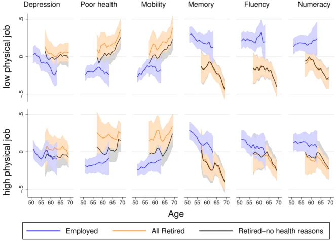
As descriptive evidence, Figure 1 plots the age profiles of average test scores by employment status, using the index estimated from model (1) to distinguish between less and more physically demanding jobs. These age-profiles have been constructed by smoothing averages by age using a 3-year centered running mean. For workers who are still employed, we do not report averages after the age of 65 because the sample size is very small. For the same reason, we do not report averages
for those retired before the age of 55.
For people in less physically demanding jobs, the figure shows large differences in health and average test scores between those who are employed and those who are retired (blue vs. orange line). Except for depression and memory, these differences are not only in the levels but also in the rates of decline with age. On the other hand, for those in more physically demanding jobs, differences are reduced (and are not statistically significant) in the case of depression and cognitive test scores.
The interpretation of the evidence presented so far may be affected by potential endogeneity of the retirement decision. To partially take this issue into account the black line considers the age profile of retired people after excluding those who report being retired for health reasons. As expected, in the case of health outcomes, health differences between employed and retired are now smaller, especially for those in more physically demanding jobs. Such descriptive analysis provides evidence of heterogeneity across occupations in the relationship between retirement and health. Moreover, once we take potential reverse causality into account, the negative correlation between retirement and health almost completely vanishes for those employed in more physically demanding jobs.
3
Identification strategy
In our estimation strategy we follow our previous work on the effect of retirement on cognition. In particular, in order to take into account the possibility of a change in the rate of decline of health after retirement, we estimate where age enters as a linear spline, namely a continuous piecewise-linear function of age, with a single knot at the reported retirement age Ri.
Specifically our baseline model (Model A) has the following form:
Hi = α0+ α1Agei+ α2DistRi+ β>Xi+ Ui, (2)
where Yi is the health status of the ith individual, Agei is her current age, DistRi = max{0, Agei−
Ri} is the number of years spent in retirement (equal to zero if the individual is not yet retired), Xi
consists of a set of indicators for country of residence (with Belgium as the reference country) and educational attainments, and Ui is a regression error potentially correlated with DistRi. Notice
that, conditional on Ui, the effect of one additional year of age on test scores is equal to α1 up
to retirement and to α1+ α2 after retirement. We also estimate a second specification (Model B)
which allows the age coefficient to be country specific (Model A plus a set of interaction terms between the linear age term and each country indicator). These models are estimated for the whole
sample and separated by gender or type of occupation (less and more physically demanding jobs) to take into account these two important sources of potential heterogeneity.
In the rest of the section we discuss a number of identification issues that arise from our identification strategy. We begin with the most important identification issue, namely potential endogeneity of the retirement decision.
3.1 Endogeneity of retirement
Endogeneity of retirement represents the main empirical challenge when trying to identify the effect of retirement on health and cognitive performance. The mean differences in Figure 1, and more generally the OLS estimates based on model 2, may be biased because of potential reverse causality (people with poor health may decide to retire earlier) or correlation between the retirement choice and unobservable factors.
As in Mazzonna and Peracchi (2012), we address the problem by using an instrumental variable (IV) strategy. Our instruments are the legislated early and normal ages of eligibility for a public old-age pension, two variables that are easily shown to be relevant and exogenous. Figures 2 and 3 present the histograms of retirement age by country, respectively for men and women. The vertical blue and red lines respectively denote the eligibility ages for early and normal retirement, while the blue and red areas indicate changes in the eligibility rules for the cohorts in our sample. The figures differ slightly from those in Mazzonna and Peracchi (2012) as we make an additional effort to increase the within country variability deriving from the many pensions reforms that took place in several European countries during the 90’s. We refer to Appendix A for further detail on pension eligibility rules in each country.
Eligibility ages differ substantially by country and gender. For instance, the early retirement age ranges from 52 in Italy before 1994 to 63 in Switzerland. Smaller cross-country and gender differences are instead observed for the normal retirement age. As aforementioned, we also exploit the within country variability that arise from the pension reforms that most of these countries undertook during the 1990’s (see also Angelini et al. 2009). Unlike previous studies (e.g. Rohwedder and Willis 2010 and Coe and Zamarro 2012), we do not use the early and normal eligibility ages at the time of the interview (2004 in our case), but the eligibility ages at the time when individuals faced their retirement decisions. Therefore, we explicitly account for changes in eligibility rules that differently affect the cohorts in the SHARE countries. To maximize correlation with our potential endogenous variable we construct our instruments in a similar way, namely as the positive part of the differences between the actual age and the legislated ages of eligibility for early and normal retirement (i.e. DistEi = max{0, Agei− Ei} and DistNi= max{0, Agei− Ni}).
3.2 Other identification issues
As argued by Bonsang et al al. (2012) and Bingley and Martinello (2013), education might be a source of bias also because cross-country differences in retirement ages are positively correlated with cross-country differences in average educational attainment. Since education is an important determinant of health and cognition later life (e.g. Mazzonna 2013), this “would invalidate the use of retirement ages as instruments without appropriate controls” (Bingley and Martinello, 2013). However, it is worth noting that, unlike Rohwedder and Willis (2010), our baseline specification does control for education and country fixed effects. Moreover, we also exploit within country variation in retirement ages that should be uncorrelated with cross-country differences in education. In MP, we discuss and test this issue along with the potential bias that might derive from cohort heterogeneity.3 However, given the importance of these issues we implement further robustness checks. In particular, we use the panel dimension of SHARE to replicate our estimates using a fixed effect approach that accounts for both endogeneity of education and cohort heterogeneity. However, we do not use this estimation strategy in the main text because of concerns with the large attrition rate across waves (33% between wave 1 and 2, almost 50% between wave 1 and 4).
Another important issue is model misspecification, namely whether the effect of retirement on health and cognition presented in equation (2) is correctly specified. This problem might be particularly important given the functional form we choose, namely a linear spline in age with a single knot at retirement. As reported in Section 5, after experimenting with polynomials of various order, we find that a linear age spline is systematically preferred by standard model selection criteria. Finally, some concerns may arise in our analysis of the heterogeneity of the effect of retirement across jobs. One concern is that people move across jobs. In particular, jobs at the end of a working life are likely to be less physically demanding than at the beginning. In our identification strategy some problems might arise if proximity to retirement, and in particular to retirement eligibility, affects an individual’s occupational choice. In Section 5 we show that our instrument is not correlated with the threshold values we use for the heterogeneity analysis and that there is no evidence in our sample of an age gradient in this occupation. However, even in the absence of bias, it is important to recognize that our analysis is limited to the last job. For instance, our analysis cannot establish whether people feel retirement as a relief because of the more recent exposure (the last job) or because the last job is a proxy for a long exposure to physically demanding jobs.
3
In cross-sectional data, the issue of cohort heterogeneity arises because age and cohort effects cannot be separately identified.
4
Empirical results
In this section we report the result from 2SLS estimates of the effect of retirement on health and cognition using the identification strategy presented in Section 3. For completeness and comparison sake, in Appendix (Tables A.1 and A.2) we also present the result from OLS estimates.
We start by showing in Table 5 the results from the first-stage regression of DistRi, the variable
that counts the years spent into retirement, on the two instruments DistEi and DistNi. The Table
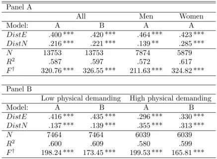
is divided in two panels. Panel A shows the results for the whole sample (both Models A and B) and separated by gender (only Model A). Panel B shows the results separated by level of physical burden measured using the internal index of physical burden described in Section 2.3. The table also shows the regression R2 and the F -test statistic for the joint significance of the excluded instruments. Our results confirm that eligibility rules are important determinants of the retirement decision. For both genders and occupational groups, and across all models, the distances from the early and normal eligibility ages are strong predictors of the distance from retirement, DistRi.
However, we can argue from our results that early retirement incentives are more important for men and for people not working in physical demanding jobs. Notice that our estimates are unaffected by the introduction, in Model B, of a country-specific linear trend in age.
Table 6 shows, for each outcome, the estimated coefficient on DistRi from the second-stage of
the 2SLS procedure. As for Panel A in Table 5, results are presented for the whole sample (both Models A and B) and separated by gender (only Model A). Starting from the pooled estimates, it is clear that retirement has a negative effect on health and cognitive abilities. For health, the magnitude of the effect is remarkably similar across outcomes. Each year into retirement increases by roughly 1% the probability of reporting 3 or more depressive symptoms, the probability of reporting poor health, and the probability of reporting 2 or more mobility limitations. These effects are quit big compared with the mean value of each indicator. They correspond to more than 5% of their means. At the same time, as we already showed in our previous work, each year into retirement decreases cognitive abilities by about 3% standard deviations or, equivalently, by 1% of their corresponding mean values. Results are also robust to the inclusion of a country-specific age trend (Model B). Finally, there is evidence of gender heterogeneity only for cognitive abilities, where point estimates are generally larger for women.
The results presented so far suggest a clear-cut answer: retirement increases the age-related rate of decline of health and cognition. The next step is to investigate whether this evidence is homogeneous across occupations. In particular, we would like to understand whether such negative effect still holds after we focus on people who used to work in more physically demanding jobs. For
this reason, we estimate model 2 separately by type of jobs, splitting the sample by the value of our internal index of physical strength. The results in Table 7 are striking. They show very clearly that the negative effect of retirement comes from people who worked in less physically demanding jobs. Heterogeneity seems to be larger for health, where the difference between the two groups is bigger and always statistically significant. In the case of cognitive abilities, confidence intervals often overlap. However, the differences in the point estimates are very large and, for people in more physically demanding jobs, the results are rarely statistically significant. It is interesting to compare the results obtained using 2SLS with the OLS estimates reported in Table A.2. In the case of OLS, the effect of retirement for people with more physically demanding jobs is not only negative and statistically significant, but is even larger than for people with less physically demanding jobs. Such apparently puzzling results may be explained by reverse causality. As already discussed in Section 2.3, those who report having retired for health reasons are concentrated in jobs that are more physically demanding.
As a robustness check, we replicate the analysis using the two external indices and splitting the sample at their mean value (physical or psycho-social index in the range 1–5 vs. 6–10). As expected, the results for the physical index are almost identical to those in Table 7. Instead, for the psycho-social index, except for the case of depression, there is no evidence of heterogeneity (results are available upon request).
The results reported so far suggest that the negative effect of retirement estimated in the whole sample disappears when we consider people working in more physically demanding job. However, such a distinction is based on the mean value of the internal index and it might be interesting to investigate whether this heterogeneity increases as we evaluate the effect on the toughest jobs. As already discussed in Section 2.3, the external indices are more suitable for this kind of analysis because of their larger support (from 1 to 10). For this reason, we estimate the effect of retirement dividing our sample into three groups depending on the value of the external index of physical burden. Specifically, we consider people with very low value of the index (1–2), people with normal value (3–8) and people with very high value (9–10). The results, presented in Table 8, show that the effect of retirement turns from negative to be positive when we focus on very physically demanding occupations. In the case of depression, poor health and numeracy the effect is statistically significant at least at 10% level despite the small number of observations for this sub-group. For people at the other extreme (very low value of the index), the negative effect of retirement seems to be larger in the case of health but smaller in the case of cognitive abilities. As a robustness check, we increase the number of people included in the high physical burden group by including also occupation with a value of the index equal to 8. The results suggest that the positive effect arises from the small
number of workers at the extreme of the index range.
Finally, to check that this heterogeneity comes only from the physical dimension of the job, we replicate the estimates using the psycho-social index. The results reported in Table 9 confirm that the effect of retirement is homogeneous when we consider the psycho-social characteristics of the jobs.
5
Robustness checks
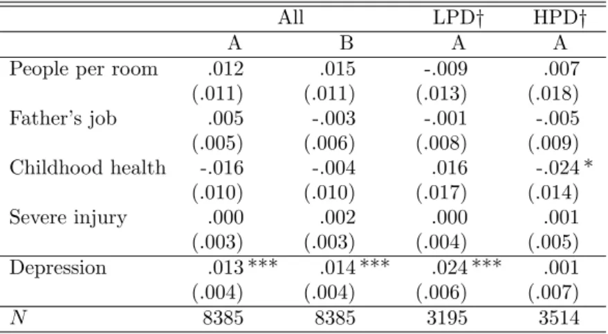
This section presents a number of checks of the robustness of our estimation strategy. Instrumental variable estimates are based on two fundamental assumptions: relevance and exogeneity. The relevance assumption can be easily tested by looking at first stage estimates shown in Table 5. The exogeneity assumption is instead untestable. In Section 3.1 and Section 3.2, we largely discuss the reasons why we think that our instruments are exogenous and we mention a large literature that supports our claim. Although untestable, such assumption can be indirectly tested by looking for instance at the effect of retirement on predetermined characteristics. If the exogeneity assumption holds, then retirement should not affect these variables.
In Table A.3, we implement this test on some predetermined characteristics collected in SHARE-LIFE, the retrospective wave of SHARE. In particular, we test whether retirement has an effect on childhood characteristics—such as childhood health, father’s occupational level, number of people per room—and on whether the respondent experience (before retirement) a severe injury that leads to disability. Unfortunately, since these information are collected 4 years after the first wave, we have a serious attrition problem that decreases the sample size of almost 40%. In order to test whether attrition compromises our testing strategy we report at the bottom of the Table the effect of retirement on depression in the same sample. The test is implemented on the whole sample (both Model A and B) and by type of job (low vs. high physically demanding jobs). The result reported in the Table shows that there is no evidence of an effect of retirement on any of the tested prede-termined characteristics under investigation. Moreover, the effect on depression is very similar to that shown in Table 6 and 7. This suggests that attrition should not alter the validity of our testing strategy. Overall, this result shows that our instruments are not correlated with important time invariant characteristics that might instead be correlated with the (endogenous) retirement choice. As anticipated in Section 3.2, this is consistent with another robustness check that we implement using the panel dimension of SHARE (waves 1 and 2). In particular, we estimate the effect of retirement using a 2SLS–fixed effect estimator founding very similar results (results available upon request).
interest. Our main concern is that the results reported so far might be only due to a small set of countries. For this reason, we also estimate separated estimates by country regions, distinguishing between Mediterranean, Continental and Scandinavian countries. The results—available upon request—show evidence of some heterogeneity across regions depending on the outcome of interest. However, there are no systematic differences across regions. Most importantly, the heterogeneity across jobs reported so far also holds when we focus on a smaller set of countries. Additionally, we replicate the estimates reported in the main text, excluding one country each time. Consistently with the previous analysis the results are robust.
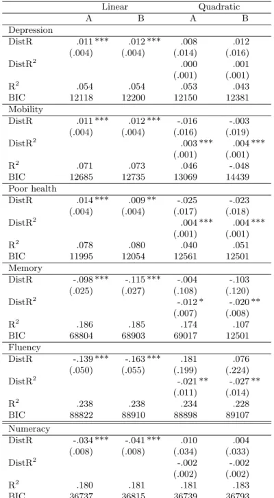
We test our basic model against alternative model specifications. In Section 4 we specify the age profile of health and cognitive abilities as a linear spine in age with a knot point at retirement. As robustness check, we experiment with polynomial of different orders. Table A.4 compares the estimates obtained using linear and quadratic splines for each outcome of interest. At the bottom of each column we report the value of the R2and the Bayesian information criteria (BIC) for model comparison. Except for numeracy, the table shows that the linear specification is always preferred by both selection criteria. It is worth noticing that in the quadratic specification, the coefficient on DistR is often positive, although never statistically significant, while the coefficient on DistR2 is negative, big and almost always statistically significant.
As anticipated in Section 3.2, the analysis of the heterogeneity of the effect of retirement across occupational groups might be affected by the fact that people at the end of their working career might move to less physically demanding job. More specifically, our analysis might be biased if the selection into the occupational groups we use in Section 4 is correlated with our instruments, the eligibility ages for early and normal retirement. In Table A.5, we show this does not occurs. In particular, the first column shows the result of a probit model for the probability of being in the high physically demanding group according to the internal index (as in Table 7); while the second and the third columns show respectively the probability of being in the very low and in the very high physically demanding group according to the external index (as in Table 8). The table shows that our two instruments do not significantly affect the probability of being in any of these groups. Most importantly, also the respondent’s age is not significantly associated with the probability of being in any of these groups. This last result is particularly important since it suggests that at least in the age window under analysis (50-70) there are not significant age related movement towards lower physically demanding jobs.
Finally, to take into account the discrete nature of our three health outcomes we replicate our estimates using a two-stage conditional maximum likelihood, instead of the standard 2SLS. The results are consistent with those reported so far.
6
Conclusions
In this paper we estimate the causal effect of retirement on health and cognitive abilities using data from 11 European countries. Unlike previous papers (Rohwedder and Willis 2010, Coe and Za-marro 2011, Bonsang et al. 2012), we take the distance from retirement into account by estimating the effect of the years since retirement. In addition, this model specification allows us to exploit both cross-country and within-country variation in early and normal retirement ages as instrument for retirement. Consistently with our previous work (Mazzonna and Peracchi 2012), the results suggest a negative effect of retirement on both health and cognitive abilities. However, we also found evidence of substantial heterogeneity across occupations. In particular the negative effect of retirement disappears as we focus on people that use to work in more physically demanding occu-pations. This effect becomes even positive when we focus on people at the top of the distribution of the physical burden associated to each occupation.
Our results are particularly relevant for policy makers who, especially in Europe, are dealing with dramatic financial crises in their social security programs. On the one hand, our results should reassure policy makers about the potential negative spillovers on health of pension reforms aimed to increase the average retirement age of the population. In fact, our results show a negative effects of early retirement on health and cognition for most of the population. On the other hand, the large heterogeneity we found across occupations suggests to take care (in designing pension policies) of people working in very physically demanding occupation—the only group for which we found some evidence of positive effect of an anticipated retirement.
References
Angelini V., Brugiavini A., and Weber G. (2009), “Ageing and unused capacity in Europe: Is there an early retirement trap?” Economic Policy, 24: 463–508.
Banks J., and Mazzonna F. (2012), “The effect of education on old age cognitive abilities: Evidence from a regression discontinuity design.” Economic Journal, 122(560):418–448.
Bingley P., and Martinello A. (2013), “Mental retirement and schooling.” European Economic Review, 63: 292–298.
Bonsang E., Adam S., and Perelman S. (2012), “Does retirement affect cognitive functioning?” Journal of Health Economics , 31(3): 490–501.
B¨orsch-Supan A., and J¨urges H. (2005), The Survey of Health, Aging, and Retirement in Europe. Method-ology. Mannheim Research Institute for the Economics of Aging (MEA).
B¨orsch-Supan A. (2013), “Myths, scientific evidence and economic policy in an aging world.” The Journal of the Economics of Ageing, 1: 3–15.
B¨orsch-Supan A., and Schuth M. (2013), “Early Retirement, Mental Health and Social Networks.” In Wise D. (ed.), Discoveries in the Economics of Aging, University of Chicago Press.
Case A., and Deaton A. (2005), “Broken down by work and sex: How our health declines.” In Wise D.A. (ed.), Analyses in the Economics of Aging, University of Chicago Press.
Charles K.K. (2004), “Is retirement depressing? Labor force inactivity and psychological well-being in later life.” Research in Labor Economics, 23: 269–299.
Coe N.B., and Zamarro G. (2011), “Retirement effects on health in Europe.” Journal of Health Economics, 30: 77–86.
d’Hombres, B., Rocco L., Suhrcke M., and McKee M. (2010), “Does social capital determine health? Evidence from eight transition countries.” Health Economics, 19: 56–74.
Folstein M.F., Folstein S.E., and McHugh P.R. (1975), “Mini-Mental State: A practical method for grading the cognitive state of patients for the clinician.” Journal of Psychiatric Research, 12: 189–198. Glass T.A., Mendes de Leon C., Marottoli R.A., and Berkman L.F. (1999), “Population based study of
social and productive activities as predictor of survival among elderly Americans.” British Medical Journal, 319: 478–483.
Glymour M.M. (2007), “When bad genes look good: APOE-e4, cognitive decline, and diagnostic thresh-olds.” American Journal of Epidemiology, 165: 1239–1246.
Grossman M. (1972), “On the concept of health capital and the demand for health.” The Journal of Political Economy, 80: 223–255.
Gruber J., and Wise D. (2004), Social Security Programs and Retirement around the World: Micro-Estimation. University of Chicago Press, Chicago.
Johnston, D.W., and Lee W.S. (2009), “Retiring to the good life? The short-term effects of retirement on health.” Economics Letters, 103(1):8–11.
Kroll L.E. (2011), “Construction and validation of a general index for job demands in occupations based on ISCO-88 and KldB-92.” Methoden – Daten – Analysen, 5: 63–90.
Mazzonna F. (2013), “The long lasting effects of education on old age health: Evidence of gender differ-ences.” Social Science and Medicine, 101: 129–138.
Mazzonna F., and Peracchi F. (2012), “Ageing, cognitive abilities and retirement.” European Economic Review, 56: 691–710.
Neuman K. (2008), “Quit your job and get healthier? The effect of retirement on health.” Journal of Labor Research, 29: 177–201.
Ravesteijn B., van Kippersluis H., and van Doorslaer E. (2013), “The contribution of occupation to health inequality.” Research on Economic Inequality, 21: 311–332.
Table 1: Sample size by country and gender.
Country Men Women AT Austria 534 503 BE Belgium 1043 674 CH Switzerland 282 230 DE Germany 863 713 DK Denmark 504 466 ES Spain 547 284 FR France 830 731 GR Greece 846 413 IT Italy 716 413 NL Netherlands 822 453 SE Sweden 887 999 Total 7874 5879
Table 2: Descriptive statistics.
Variable Mean SD Depression 0.181 0.385 Poor health 0.185 0.388 Mobility 0.195 0.396 Memory 9.132 3.255 Fluency 20.627 7.021 Numeracy 2.646 1.017 Age 59.405 5.948 Retired 0.431 0.495 High school or College 0.605 0.489
Table 3: Correlation among indices.
Internal index External (physical) External (psycho-social) Internal index 1
External (physical) 0.897 1
Table 4: Number of respondents in physical demanding jobs (internal index) by country. Country No Yes Austria 541 491 Germany 883 687 Sweden 1067 818 Netherlands 659 590 Spain 250 580 Italy 857 272 France 781 774 Denmark 493 476 Greece 685 375 Switzerland 304 208 Belgium 944 768 Total 7464 6039
Notes: This table report the distribution of physical demanding occupation index by country. The column Yes show the number of respondent in each country that work or worked in physical demanding job according to the constructed index.
Table 5: OLS estimates from the first stage regression for DistR = max{0, Age − R} by gender (Panel A) and occupation (Panel B).
Panel A
All Men Women
Model: A B A A DistE .400 *** .420 *** .464 *** .423 *** DistN .216 *** .221 *** .139 ** .285 *** N 13753 13753 7874 5879 R2 .587 .597 .572 .617 F† 320.76 *** 326.55 *** 211.63 *** 324.82 *** Panel B
Low physical demanding High physical demanding
Model: A B A B DistE .416 *** .435 *** .296 *** .330 *** DistN .137 *** .139 *** .355 *** .313 *** N 7464 7464 6039 6039 R2 .600 .609 .580 .599 F† 198.24 *** 173.45 *** 199.53 *** 165.81 ***
Notes: The table reports the result from first stage regression for DistR.
The baseline specification (Model A) includes also an age control, country fixed effects and an education dummy. Model B adds country specific age trends.
Significance levels: ***p < 0.01, **p < 0.05, *p < 0.1. Standard errors are robust to clustering at the country and cohort level. †F-test on the excluded instruments.
Table 6: Effect of retirement by gender (2SLS).
All Men Women
A B A A Depressed .010 *** .011 *** .008 ** .009 * (.003) (.003) (.004) (.005) Mobility .010 *** .012 *** .008 * .006 (.004) (.004) (.004) (.005) Poor health .011 *** .007 * .009 * .010 ** (.004) (.004) (.005) (.005) Memory -.090 *** -.112 *** .005 -.134 *** (.025) (.026) (.030) (.034) Fluency -.101 ** -.132 *** -.055 -.162 *** (.049) (.053) (.066) (.065) Numeracy -.028 *** -.034 *** -.029 *** -.034 *** (.008) (.008) (.009) (.012) N 13753 13753 7874 5879
Notes: The table reports the result from 2SLS coefficients on DistR.
The baseline specification (Model A) includes a spline in age with knot point at retirement, country fixed effects and an education dummy. Model B adds country specific age trends.
Significance levels: ***p < 0.01, **p < 0.05, *p < 0.1. Standard errors are robust to clustering at the country and cohort level.
Table 7: 2SLS. Effect of retirement by type of job (internal index).
Low physical demanding High physical demanding
A B A B Depressed .017 *** .016 *** -.000 .002 (.004) (.004) (.005) (.006) Mob. limitations .015 *** .016 *** .003 .002 (.005) (.005) (.005) (.006) Poor health .015 *** .007 * .002 -.002 (.004) (.004) (.005) (.006) Memory -.112 *** -.126 *** -.063 * -.066 (.032) (.034) (.036) (.041) Fluency -.066 -.114 -.131 ** -.073 (.062) (.070) (.066) (.073) Numeracy -.043 *** -.039 *** -.001 -.010 (.011) (.012) (.012) (.012) N 7464 7464 6039 6039
Notes: The table reports the result from 2SLS coefficients on DistR.
The baseline specification (Model A) includes a spline in age with knot point at retirement, country fixed effects and an education dummy. Model B adds country specific age trends.
Table 8: 2SLS. Effect of retirement, by physical burden (external index).
Very low (1-2) Normal (3-8) Very high (9-10) Depression .021 *** .012 *** -.014 * (.008) (.005) (.007) Mobility .007 .003 -.008 (.007) (.004) (.010) Poor health .012 * .007 -.023 ** (.007) (.004) (.011) Memory -.037 -.097 *** .068 (.056) (.031) (.079) Fluency -.037 -.111 * .094 (.118) (.062) (.170) Numeracy -.014 -.024 ** .044 * (.018) (.010) (.023) N 1785 7646 1663
Notes: The table reports the result from 2SLS coefficients on DistR as in Model B of Table 7.
The three samples are defined according to the values of the physical burden index in Kroll et al. (2011).
Significance levels: ***p < 0.01, **p < 0.05, *p < 0.1. Standard errors are robust to clustering at the country and cohort level.
Table 9: 2SLS. Effect of retirement, by psycho-social burden (external index).
Very low (1-2) Normal (3-8) Very high (9-10) Depression .014 * .011 *** .009 (.008) (.004) (.008) Mobility .002 .010 ** -.003 (.008) (.004) (.008) Poor health .003 .006 .004 (.008) (.004) (.008) Memory -.099 * -.064 ** -.127 ** (.056) (.032) (.061) Fluency .025 -.135 * -.114 (.127) (.073) (.126) Numeracy -.030 * -.006 -.031 (.017) (.010) (.020) N 1785 7646 1663
Notes: The table reports the result from 2SLS coefficients on DistR as in Model B of Table 7.
The three samples are defined according to the values of the physical burden index in Kroll et al. (2011).
Figure 2: Early and normal eligibility ages for pension benefits, by country (men). 0 .1 .2 .3 0 .1 .2 .3 0 .1 .2 .3 50 55 60 65 70 50 55 60 65 70 50 55 60 65 70 50 55 60 65 70 50 55 60 65 70 50 55 60 65 70 50 55 60 65 70 50 55 60 65 70 50 55 60 65 70 50 55 60 65 70 50 55 60 65 70 AT BE CH DE DK ES FR GR IT NL SE Early Normal
Figure 3: Early and normal eligibility ages for pension benefits, by country (women). 0 .1 .2 .3 0 .1 .2 .3 0 .1 .2 .3 50 55 60 65 70 50 55 60 65 70 50 55 60 65 70 50 55 60 65 70 50 55 60 65 70 50 55 60 65 70 50 55 60 65 70 50 55 60 65 70 50 55 60 65 70 50 55 60 65 70 50 55 60 65 70 AT BE CH DE DK ES FR GR IT NL SE Early Normal
A
Pension eligibility rules in the SHARE countries
The eligibility ages reported in our paper are the results of the country specific retirement rules that involve the cohorts in the study (born in 1934–1954) until 2004 (the first wave of SHARE). Actually, in most of these countries eligibility for early retirement also depends on work experience through the number of years of contributions. Since we do not have this information, we consider the minimum age at which an individual may have access to early retirement. For changes in the legislations, we consider the first cohort “potentially” affected (FCA). For instance, in Belgium normal retirement age for women has been gradually raised from 60 to 63: age 61 in 1997, to age 62 in 2000, and age 63 in 2003. Thus, the FCA was the 1937 cohort in 1997, the 1939 cohort in 2000, and the 1941 cohort in 2003.
Our strategy cannot perfectly predict individuals’s behavior for several reasons. First, there are additional routes to early retirement in each country (e.g. long-term unemployment, disability, plant disclosure or redundant workers). In this case, we consider the retirement program that affects the largest fraction of respondents, avoiding to consider individual characteristics that might be endogenously correlated with respondents’ health and cognition. Second, during the 90’s several countries introduced changes in the legislation that removes adverse incentive effects by moving from a ‘pay as yo go” system to less generous and more actuarially fair schemes. However, as in the case of Denmark, Germany and the Netherlands, these changes did not affect the legal early and normal retirement age. Nevertheless, these retirement ages are able to predict the most important jumps in the retirement age distribution reported in Figure 2 and 3.
The starting source of information on early and normal ages of eligibility for public old-age pen-sions in the SHARE countries is the Mutual Information System on Social Protection (MISSOC) database and the Social Security Administration (SSA) website. The MISSOC collects information on social protection for the member states of the European Union and other countries, including Switzerland. The SSA website highlights the principal features of social security programs in more than 170 countries every 2 years. These initial sources was supplemented with information from Gruber and Wise (1999, 2004, 2007), Angelini et al. (2009) and several other country specific aux-iliary data sources. Below we report the statutory old age and early retirement ages used in this paper for each country. The retirement age reported are slightly different from MP. In particular, we improve our information about past pension reforms, increasing the within country variability.
Austria
The early retirement age was 60 for men and 55 for women. The 2000 and 2003 pension reforms gradually increased the eligibility age of 2 years (step-wise increase of 2 month each quarter) for men born after September 1940 and for women born after September 1945 (see Staubli and Zweimueller 2012).
Belgium
Statutory old age retirement: for males is 65; for women was 60 but was gradually raised to 61 in 1997 (FCA 1937), 62 in 2000 (FCA 1939), and 63 in 2003 (FCA 1941).
Early retirement age: 55 for women and 60 for men.
Denmark
Statutory old age retirement : 65 for both men and women. It has been increased to 67 according to contribution requirement but it is not possible to distinguish among cohorts.
Early retirement age: 60 for both men and women.
France
In France the statutory old retirement was 65 but was lowered to 60 in 1983 for both men and women.
Early retirement age is 55 for some categories and 60 for others (we use 55 since it affected the largest share of workers).
Germany
Statutory old age retirement : from 1961, 65 for both men and women.
Early retirement age: from 1973, it is possible to have a pension with full benefits at 63 years of age (with 35 years of contribution) for men, and 60 years of age (with 15 years of contribution) for women. However, public retirement insurance pays pensions without adjustment for employees from age 60 if certain conditions are met (e.g. unemployed, part-time employed and workers who cannot be appropriately employed). As shown by Berkel and B¨orsch-Supan (2004), the interpre-tation of the laws was particularly generous, so 60 became the actual early retirement age (see also the peak in Figure 2 in particular in the East Germany. In addition, retirement before 60 was also possible mainly using unemployment compensation. With two consecutive reforms (1992 and 2001), the system was simplified and the generosity of the system dramatically decreased. In particular, after a transitional period the early retirement age was set to 63 for everybody. For women, the step-wise increase took place in 2001 reaching 62 in 2004 and 63 in 2006. For men, the
step-wise increase was heterogeneous across the categories aforementioned and affected the cohorts in this paper only marginally.
Italy
Statutory old age retirement: from 1961 to 1993, 60 (65 in the public sector) for men and 55 (60 in the public sector) for women. Several consecutive reforms (1992, 1995 and 1998) increased the statutory old age retirement to 65 for men and 60 for women with step-wise increments from 1994 to 2000.
Early retirement age: from 1965 to 1995, early retirement was possible at any age with 35 years of contributions (25 in the public sector) for both men and women; from 1996 to 2004 it was stepwise increased up to 57 for both the private and public sector.
The Netherlands
Statutory old age retirement: 65 both for men and women.
Early retirement age: At the end of the eighties the eligibility age for many early retirement schemes (including disability and unemployment) was 60 or 61 for the majority of the employees without actuarial adjustment for both men and women. Starting from the mid-1990s, several financial parameters of the early retirement schemes were changed (e.g. the contribution requirements to obtain the maximum benefit) See also Euwals, Van Vuuren and Wolthoff 2010.
Spain
Statutory old age retirement: 65 both for men and women.
Early retirement age: from 1983 to 1993, 60 for both men and women; from 1994 to 2001, 61 for both men and women; from 2002 to 2007, 61 with 30 years of contributions for both men and women.
Sweden
Statutory old age retirement: from 1961 to 1994, 67 for both men and women; from 1995 65 for both men and women.
Early retirement age: from 1961 to 1962 no early retirement; from 1963 to 1997, 60 for both men and women; from 1998 61 for both men and women.
Switzerland
Statutory old age retirement: from 1975, 65 for men and 62 for women; In 2001, women’s retirement age was raised to 63.
Early retirement age: Only since 1997 old-age insurance pensions can be claimed prior to the legal retirement age (1991 reform). In particular, men were allowed to retire at 64 from 1997 to 2001, and at 63 from 2001. For women early retirement was allowed at the age of 62 only from 2001.
Additional references for retirement ages
Berkel B., and B¨orsch-Supan A. (2004) Pension Reform In Germany: the impact on retirement decision. FinanzArchiv: Public Finance Analysis, 60(3): 393-421.
Euwals R., van Vuuren D., and Wolthoff R. (2010) “Early retirement behaviour in the Netherlands: Evi-dence from a policy reform”. De Economist 158(3): 209–236.
Gruber J., and Wise D.A. (1999) Social Security Programs and Retirement around the World. University of Chicago Press, Chicago.
Gruber J., and Wise D.A. (2007) Social Security Programs and Retirement around the World. Fiscal implications of the reform. University of Chicago Press, Chicago.
Hanel B., and Riphahn R.T. (2006) “Financial incentives and the timing of retirement: evidence from Switzerland”. IZA DP No. 2492.
Jousten A., L´efebvre M., Perelman S., and Pestieau P. (2010) “The Effects of Early Retirement on Youth Unemployment: The Case of Belgium”. In Gruber J. and Wise D.A. Social Security Programs and Retirement around the World: The Relationship to Youth Employment. University of Chicago Press, Chicago.
Social Security Administration (SSA) (2012). “Social Security Programs Throughout the World”. http://www.ssa.gov/policy/docs/progdesc/ssptw/
Staubli S., and Zweimueller J. (2012) “Does raising the early retirement age increase employment of older workers?” Journal of Public Economics, 108: 17–32.
Table A.1: OLS: Effect of retirement by gender.
All Men Women
A B A A Depressed .007 *** .007 *** .006 *** .008 *** (.001) (.001) (.001) (.002) Mob. limitations .058 *** .059 *** .051 *** .066 *** (.006) (.006) (.007) (.009) Poor health .015 *** .015 *** .015 *** .016 *** (.001) (.001) (.002) (.002) Memory -.050 *** -.049 *** -.047 *** -.051 *** (.009) (.009) (.011) (.014) Fluency -.106 *** -.102 *** -.081 *** -.142 *** (.018) (.018) (.025) (.027) Numeracy -.014 *** -.015 *** -.015 *** -.013 *** (.003) (.003) (.003) (.004) N 13753 13753 7874 5879
Notes: The table reports the result from OLS coefficients on DistR. The baseline specification (Model A) includes a spline in age with knot point at retirement, country fixed effects and an education dummy. Model B adds country specific age trends. Significance levels: ***p < 0.01, **p < 0.05, *p < 0.1. Standard errors are robust to clustering at the country and cohort level.
Table A.2: OLS: Effect of retirement by type of job.
Low physical demanding High Physical demanding
A B A B Depressed .007 *** .006 *** .008 *** .009 *** (.002) (.002) (.002) (.002) Mob. limitations .052 *** .051 *** .067 *** .070 *** (.007) (.007) (.009) (.009) Poor health .014 *** .013 *** .016 *** .017 *** (.002) (.002) (.002) (.002) Memory -.048 *** -.046 *** -.050 *** -.046 *** (.013) (.013) (.013) (.013) Fluency -.071 *** -.069 *** -.131 *** -.118 *** (.024) (.025) (.025) (.026) Numeracy -.011 *** -.011 *** -.015 *** -.017 *** (.004) (.004) (.004) (.004) N 7464 7464 6039 6039
Notes: The table reports the result from OLS coefficients on DistR. The baseline specification (Model A) includes a spline in age with knot point at retirement, country fixed effects and an education dummy. Model B adds country specific age trends. Significance levels: ***p < 0.01, **p < 0.05, *p < 0.1. Standard errors are robust to clustering at the country and cohort level.
Table A.3: Indirect exogeneity test: 2SLS Effect of retirement on predetermined characteristics.
All LPD† HPD†
A B A A
People per room .012 .015 -.009 .007 (.011) (.011) (.013) (.018) Father’s job .005 -.003 -.001 -.005 (.005) (.006) (.008) (.009) Childhood health -.016 -.004 .016 -.024 * (.010) (.010) (.017) (.014) Severe injury .000 .002 .000 .001 (.003) (.003) (.004) (.005) Depression .013 *** .014 *** .024 *** .001 (.004) (.004) (.006) (.007) N 8385 8385 3195 3514
Notes: The table reports the result from 2SLS coefficients on DistR. The baseline specification (Model A) includes a spline in age with knot point at retirement, country fixed effects and an education dummy. Model B adds country specific age trends. Significance levels: ***p < 0.01, **p < 0.05, *p < 0.1. Standard errors are robust to clustering at the country and cohort level. †LPD=Low physical demanding jobs; HPD=High physical demanding jobs.
Table A.4: Model specification (linear vs. quadratic spline): 2SLS Effect of retirement on health and cognition Linear Quadratic A B A B Depression DistR .011 *** .012 *** .008 .012 (.004) (.004) (.014) (.016) DistR2 .000 .001 (.001) (.001) R2 .054 .054 .053 .043 BIC 12118 12200 12150 12381 Mobility DistR .011 *** .012 *** -.016 -.003 (.004) (.004) (.016) (.019) DistR2 .003 *** .004 *** (.001) (.001) R2 .071 .073 .046 -.048 BIC 12685 12735 13069 14439 Poor health DistR .014 *** .009 ** -.025 -.023 (.004) (.004) (.017) (.018) DistR2 .004 *** .004 *** (.001) (.001) R2 .078 .080 .040 .051 BIC 11995 12054 12561 12501 Memory DistR -.098 *** -.115 *** -.004 -.103 (.025) (.027) (.108) (.120) DistR2 -.012 * -.020 ** (.007) (.008) R2 .186 .185 .174 .107 BIC 68804 68903 69017 12501 Fluency DistR -.139 *** -.163 *** .181 .076 (.050) (.055) (.199) (.224) DistR2 -.021 ** -.027 ** (.011) (.014) R2 .238 .238 .234 .228 BIC 88822 88910 88898 89107 Numeracy DistR -.034 *** -.041 *** .010 .004 (.008) (.008) (.034) (.033) DistR2 -.002 -.002 (.002) (.002) R2 .180 .181 .181 .183 BIC 36737 36815 36739 36793
Notes: The table reports the result from 2SLS coefficients on DistR. The baseline specification (Model A) includes a spline in age with knot point at retirement, country fixed effects and an education dummy. Model B adds country specific age trends. Significance levels: ***p < 0.01, **p < 0.05, *p < 0.1. Standard errors are robust to clustering at the country and cohort level. †LPD=Low physical demanding jobs; HPD=High physical demanding jobs.
Table A.5: Test of endogeneity of the occupational groups
Low/High Very low Very high Age -.006 -.003 .007 (.005) (.005) (.006) DistE -.018 * .011 -.001 (.010) (.012) (.014) DistN .009 .018 -.008 (.015) (.016) (.019) N 13505 11580 11580
The model also includes a dummy for female, country fixed effects and an education dummy.