General criteria for the study of quasi-stationarity

(1)

HAL Id: hal-01672979

https://hal.inria.fr/hal-01672979v2

Preprint submitted on 26 Jan 2018

HAL is a multi-disciplinary open access

archive for the deposit and dissemination of sci-entific research documents, whether they are pub-lished or not. The documents may come from teaching and research institutions in France or abroad, or from public or private research centers.

L’archive ouverte pluridisciplinaire HAL, est destinée au dépôt et à la diffusion de documents scientifiques de niveau recherche, publiés ou non, émanant des établissements d’enseignement et de recherche français ou étrangers, des laboratoires publics ou privés.

General criteria for the study of quasi-stationarity

Nicolas Champagnat, Denis Villemonais

To cite this version:

Nicolas Champagnat, Denis Villemonais. General criteria for the study of quasi-stationarity. 2017. �hal-01672979v2�

(2)

General criteria for the study of quasi-stationarity

Nicolas Champagnat1,2,3, Denis Villemonais1,2,3

January 26, 2018

Abstract

For Markov processes with absorption, we provide general criteria en-suring the existence and the exponential non-uniform convergence in to-tal variation norm to a quasi-stationary distribution. We also characterize a subset of its domain of attraction by an integrability condition, prove the existence of a right eigenvector for the semigroup of the process and the existence and exponential ergodicity of the Q-process. These results are applied to one-dimensional and multi-dimensional diffusion processes, to pure jump continuous time processes, to reducible processes with sev-eral communication classes, to perturbed dynamical systems and discrete time processes evolving in discrete state spaces.

Keywords: Markov processes with absorption; quasi-stationary distribution;

Q-process; mixing property; diffusion processes; birth and death processes; re-ducible processes; perturbed dynamical systems; Galton-Watson processes.

2010 Mathematics Subject Classification. Primary: 37A25, 60B10, 60F99, 60J05,

60J10, 60J25, 60J27; Secondary: 60J60, 60J75, 60J80, 93E03.

1 Introduction

Let (Xt, t ∈ I ) be a Markov process in E ∪ {∂} where E is a measurable space and

∂ 6∈ E, with set of time indices I which might be R+ or 1kZ+ for some k ∈ N :=

{1, 2, . . .}, whereZ+:= {0,1,...}. For all x ∈ E ∪ {∂}, we denote as usual by Px the

law of X given X0= x and for any probability measure µ on E ∪ {∂}, we define Pµ=R_{E ∪{∂}}Pxµ(dx). We also denote by Ex andEµ the associated expectations.

We assume that∂ is absorbing, which means that Xt= ∂ for all t ≥ τ∂,Px-almost

surely, where

τ∂= inf{t ∈ I , Xt= ∂}.

Our goal is to study the existence of quasi-limiting distributionsν on E for the process X , i.e. a probability measureν such that

lim

(5)

for some probability measureµ on E and for all A ⊂ E measurable. Such a mea-sureν is a quasi-stationary distribution for X , i.e. a probability measure such thatPν(Xt∈ · | t < τ∂) = ν(·) for all t ∈ I . We refer the reader to [25, 68, 82] for

general introductions on quasi-stationary distributions. In particular, it is well-known that there exists a constantλ0≥ 0 such that PνQSD(t < τ∂) = e

−λ0t _{for all}

t ∈ I .

More precisely, our first goal is to give general criteria involving Lyapunov-type functionsϕ1andϕ2ensuring the existence of a quasi-stationary distribu-tionνQSDsuch that

°

°Pµ(Xt∈ · | t < τ∂) − νQSD°°_{T V} ≤ C αt

µ(ϕ1)

µ(ϕ2)

, ∀t ∈ I , (1.1)

for some constants C ∈ (0,+∞) and α ∈ (0,1) and for all probability measure µ on E such thatµ(ϕ1) < +∞ and µ(ϕ2) > 0, where µ(ϕ) :=REϕ(x)µ(dx). Here, the

total variation distance is defined as

kµ1− µ2kT V = sup f :E →[−1,1] measurable

|µ1( f ) − µ2( f )|.

This measureνQSD is the only quasi-stationary distributionν such that ν(ϕ1) < +∞ and ν(ϕ2) > 0. Our second goal is to show how our criteria can be ap-plied to a wide range of Markov processes, including several classes of processes for which even the existence of a quasi-stationary distribution was not known, such as diffusions in irregular domains or perturbed dynamical systems in un-bounded domains.

General criteria ensuring that the convergence in (1.1) holds uniformly with respect to the initial distributionµ have been studied in [6, 15]. In this case, νQSD

is the quasi-limiting distribution of any initial distributions. However, these re-sults do not apply to processes admitting several quasi-stationary distributions, which is known to happen in a variety of specific cases, even for processes ir-reducible in E (including branching processes [77, 2, 60, 63], one-dimensional birth and death processes [80, 37, 36, 85] and one-dimensional diffusion pro-cesses [62, 66]). In addition, as for non-absorbed propro-cesses, uniform conver-gence with respect to the initial distribution only happens for processes that come back quickly in compact sets [69, 15] or are killed fast [83]. The present pa-per provides general criteria generalizing those of [15] to cases of non-uniform convergence and, contrary to the above cited references, does not assume that Px(t < τ∂) > 0 for all x ∈ E and all t ∈ I .

Given a quasi-stationary distributionν, its domain of attraction is defined as the set of probability measuresµ on E such that P_µ(Xt∈ · | t < τ∂) converges

(6)

contains all Dirac masses,ν is called the Yaglom limit, or the minimal

quasi-stationary distribution. In all the models admitting several quasi-quasi-stationary

tributions cited above, it has been proved that the minimal quasi-stationary dis-tribution exists. The convergence (1.1) implies in addition that the domain of attraction of the Yaglom limitνQSD actually contains all measuresµ such that

µ(ϕ1) < ∞ and µ(ϕ2) > 0.

Our first step is to provide criteria ensuring (1.1) for all t ∈ Z+. We also obtain several consequences, including a larger set of initial distributions be-longing to the domain of attraction ofνQSD and a geometric convergence for

a stronger norm than the total variation. We also prove the geometric conver-gence in L∞(ϕ1) of x 7→ eλ0nPx(n < τ∂) as n → +∞ to a function η satisfying

Ex(η(Xn)1n<τ∂) = eλ0nη(x) for all n ∈ Z+ and x ∈ E, and deduce a spectral gap property for the semigroup of the absorbed process (Xn, n ∈ Z+). Finally, we also obtain the existence of the process (Xn, n ∈ Z+) conditioned to never be absorbed (the so-called Q-process) and its geometric ergodicity (we refer the reader to [1] and references therein for general considerations on the link be-tween Q-processes and quasi-stationary distributions through theα-theory of general Markov chains). All these results are stated in Section 2 and proved in Sections 9 and 10.

The last criterion assumes that (Xn, n ∈ Z+) is aperiodic but of course applies to 1-periodic processes (Xt, t ∈ I ). Under additional aperiodicity assumptions,

we show in Section 3 how the previous results extend to general time indices t ∈ I and provide practical versions of our criteria for continuous-time processes. We also provide simple criteria allowing to check our conditions and show that the known criteria for uniform convergence in (1.1) obtained in [15] can be recov-ered using our approach. The results of this section are proved in Section 11.

These results allow us to put in a unified framework a large body of works on quasi-stationary distributions as illustrated by the rest of the paper, which is devoted to the application of our abstract criteria. We start in Section 4 with diffusion processes inRd, d ≥ 1, absorbed at the boundary of a domain D. Our analysis provides for example the following general result.

Theorem 1.1. Assume that E = D is a bounded connected open subset of Rdand that (Xt, t ∈ R+) is solution to

d Xt= b(Xt)d t + σ(Xt)d Bt

until its first exit timeτ_∂from D, where B is a r -dimensional Brownian motion and b :Rd → Rd andσ : Rd → Rd ×r are Hölder functions, such that σ is uni-formly elliptic. Then, the process X has a unique quasi-stationary distribution

(7)

νQSDwhich satisfies ° °Pµ(X_t∈ · | t < τ∂) − ν_QSD ° °_{T V}≤ 1 µ(ϕ2)α t , ∀t ∈ [0,+∞)

for some positive functionϕ2on D and a constantα ∈ (0,1). In addition, there

exists a positive, boundedC2(D) functionη such that

d X i =1 bi(x)∂η ∂xi(x) + 1 2 d X i , j =1 r X k=1 σi k(x)σj k(x) ∂ 2_η ∂xi∂xj(x) = −λ0η(x), ∀x ∈ D and η(x) = lim t →+∞e λ0tP x(t < τ∂), ∀x ∈ D,

where the convergence is uniform in D.

We emphasize that one of the main contributions of this result with respect to the existing literature (see for example [73, 42, 10, 57, 33, 12, 18]) is that it applies to any bounded domain D without any regularity assumption. Theo-rem 1.1 is in fact obtained in Section 4 as a particular case of a criterion for unbounded domains and coefficients b andσ only locally Hölder and locally uniformly elliptic in D. We also consider the case of diffusions with killing in Section 4.4. All these results are proved in Section 12.

Absorbed one-dimensional diffusions with or without killing have received a lot of attention (see for instance [64, 24, 62, 66, 78, 9, 61, 58, 48, 71, 19, 17]). We consider these models in Section 4.5. Our main contributions with respect to the literature are the characterization of a larger subset of the domain of attraction of the minimal quasi-stationary distribution, weaker regularity of the drift and diffusion coefficients and explicit general bounds onϕ1andλ0allowing to check our criteria.

The case of continuous-time Markov processes in discrete state spaces is considered in Section 5 with application to multitype birth and death processes absorbed at the exit of any connected E ⊂ Zd₊(in the sense of the nearest neigh-bors structure ofZd₊). Note that the quasi-stationary behavior of finite state space processes [29] and of one-dimensional birth and death processes [54, 43, 11, 55, 80, 81] has been extensively studied using spectral methods that do not generalize easily to the multi-dimensional countable state-space setting. The quasi-stationary behavior of multi-dimensional birth and death processes was studied in the case of uniform convergence in (1.1) in [16, 18, 22, 23].

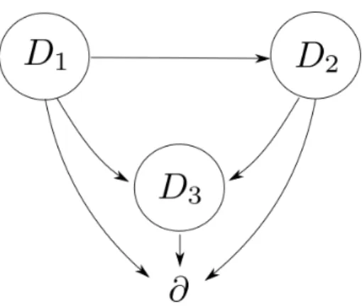
All the previous examples assumed irreducibility of X in E . In Section 6, we show that our criteria also apply to reducible cases, as those considered in [72]

(8)

(for Galton-Watson processes), [44] (for discrete processes), [14] (for Feller dif-fusions) and [13, 82] (in the finite case). We first give a general criterion in Sub-section 6.1 and we study in details an example with a countable infinity of com-munication classes in Subsection 6.2.

In Section 7, we consider general models in discrete time and continuous space, first extending the criteria of [6, 12] in order to cover the case of Euler schemes for stochastic differential equations absorbed at the boundary of a do-main (as defined in [65, 40]) and penalized semigroups (as in [31, 32]; note that all our results naturally extend to penalized homogeneous semigroups, provided the penalization rate is bounded from above, see [20]). We then study in de-tails the case of perturbed dynamical systems, as those considered for example in [5, 4, 49], where the quasi-stationary behavior was studied using the criterion of [6]. As an illustration of our method, let us mention the following original result.

Theorem 1.2. Let D be a measurable set ofRd with positive Lebesgue measure and let∂ 6∈ D. Assume that

X_n+1= (

f (Xn) + ξn if Xn6= ∂ and f (Xn) + ξn∈ D,

∂ otherwise,

where f :Rd→ Rdis a locally bounded measurable function such that

|x| − | f (x)| −−−−−−→ |x|→+∞ +∞

and (ξn)n∈N is an i.i.d. non-degenerate Gaussian sequence inRd. Then (1.1) is

satisfied forϕ1(x) = e|x|and a positive measurable functionϕ2on D.

Finally, we study in Section 8 the case of processes in discrete time and dis-crete space. This is the most studied situation in the literature since it cov-ers both the Galton-Watson processes [88, 46, 51, 2] and the general discrete case [28, 77, 37, 38, 36, 35, 44, 67]. We first show in Subsection 8.1 that our results allow to recover the general criterion of [35], based on the theory of R-positive matrices. We then consider general population processes dominated by population-dependent multi-type Galton-Watson processes in Subsection 8.2. The case of population-dependent Galton-Watson processes with a single type was studied in [44] using quasi-compactness methods. We also obtain as a corol-lary results on subcritical multi-type Galton-Watson processes. We do not re-cover the optimal L log L assumption on the offspring distribution [51, 47] for the existence of a minimal quasi-stationary distributionνQSD having finite first

moment, but we obtain a stronger form of convergence in (1.1), a larger subset of its domain of attraction and stronger moments properties onνQSD.

(9)

2 Main Results

Let (Xt, t ∈ I ) be a Markov process in E ∪ {∂} where E is a measurable space and

∂ 6∈ E, with set of time indices I which might be Z+= {0, 1, . . .}, R+ or k1Z+ for some k ∈ N = {1,2,...}. We define the absorption time τ∂as

τ∂= inf{t ∈ I , Xt= ∂}.

In this section, we study the sub-Markovian transition semigroup of X consid-ered at integer times, (Pn)n∈Z+, defined as

Pnf (x) = Ex¡ f (Xn)1n<τ∂¢ , ∀n ∈ Z+,

for all bounded or nonnegative measurable function f on E and all x ∈ E. We also define as usual the left-action of Pnon measures as

µPnf = Eµ¡ f (Xn)1n<τ∂¢ =

Z

E

Pnf (x)µ(dx),

for all probability measureµ on E and all bounded measurable f . We make the following assumption.

Assumption (E). There exist positive integers n1and n2, positive real constants

θ1,θ2, c1, c2, c3, two functionsϕ1,ϕ2: E → R+ and a probability measureν on a measurable subset K ⊂ E such that

(E1) (Local Dobrushin coefficient). ∀x ∈ K ,

Px(Xn1∈ ·) ≥ c1ν(· ∩ K ).

(E2) (Global Lyapunov criterion). We haveθ1< θ2and inf x∈Eϕ1(x) ≥ 1, sup_x∈Kϕ1(x) < ∞ inf x∈Kϕ2(x) > 0, sup_x∈Eϕ2(x) ≤ 1, P1ϕ1(x) ≤ θ1ϕ1(x) + c21K(x), ∀x ∈ E P1ϕ2(x) ≥ θ2ϕ2(x), ∀x ∈ E . (E3) (Local Harnack inequality). We have

sup

n∈Z+

sup_y∈KPy(n < τ∂)

(10)

(E4) (Aperiodicity). For all x ∈ K , there exists n4(x) such that, for all n ≥ n4(x),

Px(Xn∈ K ) > 0.

Note that it follows from (E2) thatθ2≤ 1 and thus θ1< 1.

In Section 3, criteria implying (E) and adapted to the continuous time setting are provided. Several examples of Markov processes satisfying this assumption are provided in Sections 4 to 8.

In the rest of this section, we state our main results. We start with the expo-nential contraction in total variation of the conditional marginal distributions of the process given non-absorption. Its proof is given in Section 9.

Theorem 2.1. Assume that Condition (E) holds true. Then there exist a constant

C > 0, a constant α ∈ (0,1), and a probability measure νQSDon E such that

° ° ° ° µPn µPn1E − νQSD ° ° ° ° T V ≤ C αnµ(ϕ1) µ(ϕ2) , (2.1)

for all probability measureµ on E such that µ(ϕ1) < ∞ and µ(ϕ2) > 0. Moreover,

νQSDis the unique quasi-stationary distribution of X that satisfiesνQSD(ϕ1) < ∞

andνQSD(ϕ2) > 0. In addition νQSD(K ) > 0.

Note thatµ(ϕ2) > 0 and (E2) imply that µPnϕ2> 0 and hence µPn1E> 0 for

all n ∈ N. Hence the left-hand side of (2.1) is well-defined.

Remark 1. The last result characterizes a subset of the domain of attraction of νQSD, defined here as the set of probability measuresµ on E such that Pµ(Xn∈

· | n < τ∂) converges toνQSD in total variation when n → +∞. Note that, for a

given semigroup (Pn), different choices ofϕ1(andϕ2) satisfying Assumption (E) can lead to bigger subsets of the domain of attraction. In particular, observing that, for all p ≥ 1, Hölder’s inequality entails

P1(ϕ1/p₁ ) ≤ (θ1ϕ1+ c21K)1/p≤ θ1/p₁ ϕ1/p₁ + c2(p)1K

with c2(p) := (1 + c2/θ2)1/p− 1, we see that (ϕ1/p1 ,ϕ2) satisfies Assumption (E) for all p < logθ1/ logθ2. Therefore, the domain of attraction ofνQSD actually

contains any probability measureµ such that µ(ϕ2) > 0 and µ(ϕ1/p₁ ) < ∞ for some p < logθ1/ logθ2.

In Theorem 2.1, we obtain an exponential rate of convergence in total varia-tion, uniform with respect to initial distributionsµ such that µ(ϕ1)/µ(ϕ2) ≤ A for any constant A. As will appear in applications, the functionϕ2may have com-pact support, and henceµ(ϕ2) could vanish for a large set of initial measures

(11)

µ. However, the convergence toward the quasi-stationary distribution νQSDcan

happen for such measures. The next result shows that it is the case as soon as

µ(ϕ1) < ∞ and the process can reach K under Pµ, that is ifµ(E0) > 0 where

E0:= {x ∈ E : ∃k ≥ 0 s.t. Pk1K(x) > 0}.

In fact,

E0=©x ∈ E : ∃k ≥ 0 s.t. Pkϕ2(x) > 0ª . (2.2) To prove this, we first observe that E0⊂©x ∈ E : ∃k ≥ 0 s.t. Pkϕ2(x) > 0ª sinceϕ2 is positive on K . For the converse inclusion, we notice that TK:= inf{n ∈ Z+, Xn∈

K } is infinitePx-almost surely for all x ∈ E \ E0. Hence it follows from (E2) that

Px(n < τ∂) ≤ Ex£1n<τ∂ϕ1(Xn)¤ ≤ θn1ϕ1(x) for all n ≥ 1 for such x. Since in addi-tion (E2) entails thatPx(n < τ∂) ≥ Ex

£

1n<τ∂ϕ2(Xn)¤ ≥ θn2ϕ2(x) and sinceθ1< θ2, we deduce thatϕ2(x) = 0, and hence (2.2) is proved.

The next result follows immediately from Theorem 2.1 considering as initial distribution the probability measureµPk/µPk1E.

Corollary 2.2. Assume that Condition (E) holds true. Consider any probability

measureµ on E such that µ(E0) > 0 and µ(ϕ1) < ∞. Then there exists k ≥ 0 such

thatµPkϕ2> 0 and ° ° ° ° µPn µPn1E− ν QSD ° ° ° ° T V ≤ C αn−kµPkϕ1 µPkϕ2 , ∀n ≥ k, (2.3)

where the constants C and α and the measure νQSD are the same as in

Theo-rem 2.1.

Remark 2. Conversely, ifµ(E0) = 0, then Pµ(Xn∈ K | n < τ∂) = 0 for all n ≥ 0.

SinceνQSD(K ) > 0, we cannot have convergence in total variation of Pµ(Xn ∈

· | n < τ∂) toνQSD. Hence the domain of attraction ofνQSD does not contain

measuresµ such that µ(E0) = 0. Examples where E 6= E0will be given in Section 6. In particular, combining Remark 1 and Corollary 2.2, we obtain the following subset of the domain of attraction ofνQSD.

Corollary 2.3. Assume that Condition (E) holds true. Then the domain of

attrac-tion ofνQSDcontains all the probability measuresµ on E such that µ(E0) > 0 and

µ(ϕ1/p1 ) < ∞ for some p < logθ1/ logθ2.

Note that, ifϕ1is bounded and E0= E, there exists a unique quasi-stationary distribution which attracts all the initial distributions.

The above results deal with convergence in total variation. We actually ob-tain a stronger notion of convergence, proved in Section 10.2. Note that the proof makes use of our next result Theorem 2.5, proved in Section 10.1.

(12)

Theorem 2.4. Assuming that Condition (E) holds true, for any p ∈ [1,logθ1/ logθ2),

there existαp< 1 and a finite constant Cpsuch that, for all probability measure

µ on E such that µ(ϕ1/p1 )/µ(ϕ2) < ∞ and for all real function h on E such that |h| ≤ ϕ1/p1 , ¯ ¯Eµ[h(X_n) | n < τ∂] − ν_QSD(h) ¯ ¯≤ C_p µ(ϕ1/p1 ) µ(ϕ2) α n p. (2.4)

This result easily extends as in Corollary 2.2.

We also obtain under Condition (E) the asymptotic behavior of the absorp-tion probabilities and an eigenfuncabsorp-tion of P1for the eigenvalueθ0, whereθ0∈ (0, 1] is such that

PνQSD(n < τ∂) = θ

n

0, ∀n ∈ N.

We recall that the existence ofθ0is a classical general result for quasi-stationary distributions [68]. Note that, ifτ_∂< ∞ with positive Px-probability for all x ∈ K ,

θ0< 1 and in this case, absorption occurs in finite time PνQSD-almost surely. The

caseθ0= 1 corresponds to the case where τ∂= ∞ PνQSD-almost surely. Because

of the next Theorem 2.5, under Condition (E), this will occurs if and only if there exists x ∈ E such that τ∂= +∞ Px-almost surely.

To state this result, we define for all positive functionψ on E the space L∞(ψ) as the set of real functions f on E such that kf kL∞₍_ψ):= sup_x∈E f (x)/ψ(x) < ∞.

Note that (L∞(ψ),k · kL∞₍_ψ)) is a Banach space.

Theorem 2.5. Assume that Condition (E) holds true. Then, there exists a function

η : E → R+such that η(x) = lim n→+∞ Px(n < τ∂) PνQSD(n < τ∂) = lim n→+∞θ −n 0 Px(n < τ∂), ∀x ∈ E , (2.5)

where the convergence is geometric in L∞(ϕ1/p₁ ) for all p ∈ [1,logθ1/ logθ0). In

addition, inf_y∈Kη(y) > 0, E0= {x ∈ E : η(x) > 0}, νQSD(η) = 1,

P1η = θ0η and θ0≥ θ2> θ1.

Note that the last result implies that, whenη is bounded, one can actually takeϕ2= η/kηk∞in Condition (E2).

Theorem 2.5 implies thatθ0is an eigenvalue for P1in L∞(ϕ1) and that the associated eigenfunctionη belongs to L∞(ϕ1/p₁ ) for all p < logθ1/ logθ0. The next result, proved in Section 10.3, shows a spectral gap betweenθ0and the next eigenvalue and that, actually,η ∈ L∞³ϕlogθ0/ logθ1

1

´ .

(13)

Corollary 2.6. Assume that Condition (E) holds true and let ˆP1f (x) = Exf (X1)

for all x ∈ E ∪ {∂} and f : E ∪ {∂} → R in L∞(1{∂}+ ϕ1). Then each eigenfunction

h ∈ L∞(1{∂}+ϕ1) (possibly with complex values) of ˆP1for an eigenvalueθ (possibly

belonging toC) satisfies the following properties:

1. if h(∂) 6= 0 and if Px(τ∂< ∞) = 1 for all x ∈ E, then h is constant;

2. if h(∂) = 0, if there exists x ∈ E0_{such that h(x) 6= 0 and if ν}

QSD(h) 6= 0, then

h = νQSD(h)η and θ = θ0(with the conventionη(∂) = 0);

3. if h(∂) = 0, if there exists x ∈ E0_{such that h(x) 6= 0 and if ν}

QSD(h) = 0, then

|θ| ≤ θ0α1, whereα1< 1 is the constant of Theorem 2.4;

4. if h(∂) = 0 and h(x) = 0 for all x ∈ E0, thenνQSD(h) = 0 and |θ| ≤ θ1.

In addition, if |θ| > θ1(which can only happen in cases 2. and 3. above), then there

exists a constant C such that

|h(x)| ≤ C ϕ1(x)log |θ|/logθ11E0(x), ∀x ∈ E . (2.6)

We end this section with the study of the Q-process and its ergodicity prop-erties under Condition (E). In the next result, proved in Section 10.4,Ω = EZ+_is

the canonical state space of Markov chains on E and (Fn)n∈Z+is the associated

canonical filtration.

Theorem 2.7. Condition (E) implies the following properties.

(i) Existence of the Q-process. There exists a family (Qx)x∈E0of probability

mea-sures onΩ defined by

lim

n→+∞Px(A | n < τ∂) = Qx(A)

for all x ∈ E0, for allFm-measurable set A and for all m ≥ 0. The

pro-cess (Ω,(Fm)m≥0, (Xn)n≥0, (Qx)x∈E0) is an E0-valued homogeneous Markov

chain.

(ii) Semigroup. The semigroup of the Markov process X under (Qx)x∈E0 is given

for all bounded measurable functionϕ on E0and n ≥ 0 by

e

Pnϕ(x) =

θ−n 0

(14)

(iii) Exponential ergodicity. The probability measureβ on E0defined by β(dx) = η(x)νQSD(d x).

is the unique invariant distribution of the Markov process X under (Qx)x∈E0.

Moreover, for any p ∈ [1,logθ1/ logθ2), there exist constants Cp> 0 andαep∈ (0, 1) such that, for all initial distributionsµ on E0_{such that}_µ(ϕ1/p

1 /η) < ∞

and for all measurable real function h on E0such that |h| ≤ ϕ1/p1 /η, ¯ ¯EQ_µ[h(X_n)] − β(h) ¯ ¯≤ C e αn pµ ³ ϕ1/p1 /η ´ , ∀n ≥ 0, (2.8)

whereQ_µ=RE0Qxµ(dx). In addition, for all initial distributions µ on E0,

°

°µPen− β

°

°_{T V} −−−−→

n→∞ 0. (2.9)

3 Other formulations and particular cases of Assumption (E)

In this section, we provide general comments on Assumption (E). Basic facts are gathered in Subsection 3.1, Subsection 3.2 focuses on criteria adapted to contin-uous time processes and we consider the case of uniform convergence in Theo-rem 2.1 in Subsection 3.3.

3.1 General comments on the assumptions

When Conditions (E2) and (E4) are satisfied, one can use comparison techniques on transition probabilities in order to check that Conditions (E1) and (E3) hold true, as stated in the following proposition, proved in Subsection 11.1.

Proposition 3.1. Assume that Conditions (E2) and (E4) are satisfied and that

there exist two constants C > 0 and n0≤ m0∈ N such that

Px(Xn0∈ · ∩ K ) ≤ C Py(Xm0∈ ·), ∀x ∈ E and y ∈ K . (3.1)

Then Condition (E) is satisfied. Moreover, there exists a constant C0_{> 0 such that,}

for all x ∈ E and all n ≥ 0,

Px(n < τ∂) ≤ C0ϕ1(x) inf

y∈KPy(n < τ∂).

In order to prove the existence of functionsϕ1 and ϕ2 in Condition (E2), one may use probabilistic properties of the Markov process X , as stated by the following lemmas, proved in Sections 11.2 and 11.3. The first lemma shows how to constructϕ2.

(15)

Lemma 3.2. Let K be a measurable subset of E . If there existsθ2> 0 such that inf x∈Kθ −n 2 Px(Xn∈ K ) −−−−−→ n→+∞ +∞,

then the functionϕ2: E → [0,1] defined by ϕ2(x) = θ

−1 2 −1 θ−` 2 −1 P`−1 k=0θ−k2 Px(Xk ∈ K ),

where` is such that θ−`₂ inf_x∈KPx(X`∈ K ) ≥ 1, verifies infKϕ2> 0 and P1ϕ2(x) ≥

θ2ϕ2(x). Moreover, it implies that (E4) is satisfied.

The second lemma shows how to construct ϕ1. We define TK = inf{n ≥

0, Xn∈ K }.

Lemma 3.3. Let K be a measurable subset of E . If there exists a constantθ1> 0

such that Ex ³ θ−TK∧τ∂ 1 ´ < +∞ ∀x ∈ E and C := sup y∈K E y ³ EX1 ³ θ−TK∧τ∂ 1 ´ 11<τ∂ ´ < +∞,

then the functionϕ1: E → [1,+∞) defined by ϕ1(x) = Ex

³ θ−TK∧dτ∂e 1 ´ satisfies sup K ϕ1< +∞ and P1ϕ1≤ θ1ϕ1+C1K.

Conversely, if there exist two constants C > 0, θ1 > 0 and a function ϕ1 : E → [1, +∞) such that supKϕ1< +∞ and P1ϕ1≤ θ1ϕ1+ C1K, then, for allθ > θ1,

there exists a constant C_θsuch that

Ex¡θ−TK∧τ∂¢ ≤ Cθϕ1(x) ∀x ∈ E and sup y∈KE y¡EX1 ¡ θ−TK∧τ∂¢ 11<τ∂¢ < +∞.

As many results of Section 2 make use of the functionϕ1/p₁ with a parame-ter p ∈ [1,logθ1/ logθ2), it is important to characterize the best possible value of

θ2. The following lemma shows that the domain of attraction provided by Corol-lary 2.3 can be taken as the set of probability measuresµ on E such that µ(E0) > 0 andµ(ϕ1/p) < ∞ for some p < logθ1/ logθ0. This result is proved in Section 11.4. Lemma 3.4. If Condition (E) is satisfied for some functionsϕ1andϕ2with

con-stantsθ1andθ2, then, for allθ₂0 ∈ (θ1,θ0) it is also satisfied forϕ1and some

func-tionϕ0₂with constantsθ1andθ02.

In many general studies of quasi-stationary distributions [68, 15], one usu-ally assumes thatPx(τ∂< ∞) = 1 for all x ∈ E (so that the conditioning becomes singular in the limit of large time) andPx(n < τ∂) > 0 for all n > 0 and all x ∈ E so

(16)

that the conditioning is well-defined for all finite time t . The results of Section 2 are true without assuming these two conditions.

For the first one, if we assume thatτ_∂= ∞ Px-almost surely for all x ∈ E,

then Condition (E3) becomes void and one can takeϕ2≡ 1 in (E2), so that θ2=

θ0= 1. We recognize in (E1) the standard “small set” assumption of [70], in the condition (E2) forϕ1a standard Foster-Lyapunov criterion and condition (E4) is an aperiodicity condition.

For the second one, under Condition (E), their may exist points x ∈ E \ E0 such thatPx(n < τ∂) = 0 for some n > 0. However, for all x ∈ E0, there exists

k ∈ N such that Pk1K(x) > 0. Hence, for all n ≥ k, Pn1E(x) ≥ Pk(Pn−kϕ2)(x) ≥

θn−k

2 infKϕ2Pk1K(x) > 0. In particular, for all µ such that µ(E0) > 0, µPn1E> 0

for all n ≥ 0 and thus, the conditional distribution in the left-hand side of (2.3) is well-defined.

3.2 On continuous time

In Section 2, we only considered the conditional behavior of the process X at integer times. In general, the results of Section 2 do not give information about the process at intermediate times. In this section, we derive a sufficient condi-tion which is well suited for continuous time Markov processes or for aperiodic Markov processes. We consider an absorbed Markov process (Xt)t ∈I with time

parameter in I = Z+or [0, +∞).

Assumption (F). There exist positive real constantsγ1,γ2, c1, c2and c3, t1, t2∈

I , a measurable functionψ1: E → [1,+∞), and a probability measure ν on a measurable subset L ⊂ E such that

(F0) (A strong Markov property). Defining

τL:= inf{t ∈ I : Xt∈ L}, (3.2)

assume that for all x ∈ E, XτL∈ L, Px-almost surely on the event {τL< ∞}

and for all t > 0 and all measurable f : E ∪ {∂} → R+,

Ex£ f (Xt)1τL≤t <τ∂¤ = Ex h 1τL≤t ∧τ∂EXτL£ f (Xt −u)1t −u<τ∂ ¤ u=τL i .

(F1) (Local Dobrushin coefficient). ∀x ∈ L,

(17)

(F2) (Global Lyapunov criterion). We haveγ1< γ2and Ex(ψ1(Xt2)1t2<τL∧τ∂) ≤ γ t2 1ψ1(x), ∀x ∈ E Ex(ψ1(Xt)1t <τ∂) ≤ c2, ∀x ∈ L, ∀t ∈ [0, t2] ∩ I , γ−t 2 Px(Xt∈ L) −−−−→ t →+∞ +∞, ∀x ∈ L.

(F3) (Local Harnack inequality). We have

sup

t ≥0

sup_y∈LPy(t < τ∂)

inf_y∈LPy(t < τ∂) ≤ c3

The following result is proved in Section 11.5.

Theorem 3.5. Under Assumption (F), (Xt)t ∈Iadmits a quasi-stationary

distribu-tionνQSD, which is the unique one satisfyingνQSD(ψ1) < ∞ and PνQSD(Xt∈ L) > 0

for some t ∈ I . Moreover, there exist constants α ∈ (0,1) and C > 0 such that, for all probability measuresµ on E satisfying µ(ψ1) < ∞ and µ(ψ2) > 0,

° °Pµ(X_t∈ · | t < τ∂) − ν_QSD ° °_{T V} ≤ C αt µ(ψ1) µ(ψ2), ∀t ∈ I , (3.3)

whereψ2(x) =Pn_k=00 γ₂−kt2Px(Xkt2∈ L) for n0≥ 1 large enough. In addition, there

exists a constantλ0≥ 0 such that λ0≤ log(1/γ2) < log(1/γ1) andPνQSD(t < τ∂) =

e−λ0t_{for all t ≥ 0, and there exists a function η such that}

η(x) = lim

t →+∞e λ0tP

x(t < τ∂), ∀x ∈ E , (3.4)

where the convergence is exponential in L∞(ψ1/p₁ ) for all p ∈ [1,log(1/γ1)/λ0),

and Ptη(x) = e−λ0tη(x) for all x ∈ E and t ≥ 0.

In particular, if I = R+andη is bounded,setting η(∂) = 0, the function η de-fined on E ∪{∂} belongs to the domain of the infinitesimal generator L of X and L η = −λ0η.

Remark 3. We shall actually prove that Assumption (F) implies that

Assump-tion (E) is satisfied for the sub-Markovian semigroup (Pn)n≥0 of the absorbed

Markov process (Xnt2)n∈Z+, with the functionsϕ1= ψ1andϕ2=

γ−t2 2 −1

γ−(n0+1)t2

2 −1

ψ2, anyθ1∈ (γt₁2,γ₂t2),θ2= γ₂t2and the set

K =© y ∈ E, Py(τL≤ t2)/ψ1(y) ≥ (θ1− γ₁t2)/c2ª ⊃ L.

In particular, all the consequences of (E) stated in Section 2 hold true. More-over, on can also obtain a continuous-time version of Theorem 2.7 about the

(18)

Remark 4. For continuous-time Markov processes, a classical Foster-Lyapunov

inequality (cf. [70]) involving the infinitesimal generatorL of the process X is given by

L ψ1(x) ≤ −λ1ψ1(x) +C1K(x), ∀x ∈ E . (3.5)

Equation (3.5) implies (formally, assuming one can apply Dynkin’s formula) that Ex[11≤τL∧τ∂ψ1(X1)] ≤ e−λ1ψ1(x) andEx[ψ1(Xt)1t <τ∂] ≤ eC tψ1(x), so that the first

two lines of (F2) can be deduced. However, it is not possible to directly check (E2) forϕ1= ψ1from (3.5). This explains the specific form we choose for the first and second lines of (F2), and the Foster-Lyapunov criteria that will be used for diffusions in Section 4 and for pure jump processes in discrete state space in Section 5. Note that a functionψ1satisfying (3.5) usually does not belong to the domain of the infinitesimal generatorL , so one needs to extend the notion of infinitesimal generator as in [70, 18].

As in the discrete time setting, one can use controls on the exponential mo-ments for the return times in L instead of using Lyapunov type functionsψ1. The following result is proved in Section 11.6.

Lemma 3.6. Assume that there exist positive constantsγ1> 0 and t2∈ I such that Ex ¡ γ−τL∧τ∂ 1 ¢ < ∞, ∀x ∈ E and sup x∈LEx ³ EX_t2 ¡ γ−τL∧τ∂ 1 ¢´ < +∞, thenψ1(x) = Ex¡γ−τ₁ L∧τ∂¢ satisfies Ex(ψ1(Xt2)1t2<τL∧τ∂) ≤ γ t2 1ψ1(x), ∀x ∈ E Ex(ψ1(Xt)1t <τ∂) ≤ c2, ∀x ∈ L, ∀t ∈ [0, t2] ∩ I ,

for some constant c2> 0.

3.3 The case of uniform exponential convergence

Let us now come back to the general case of Section 2. Note first that, in the case where (E) is satisfied with a bounded functionϕ1, because of Corollary 2.3, the domain of attraction ofνQSDcontains all the probability measuresµ on E such

thatµ(E0) > 0. The next result hence follows from Remark 2.

Proposition 3.7. If Condition (E) is satisfied with a bounded functionϕ1, then

νQSD is the unique quasi-stationary distribution of (Xn) giving positive mass to

E0and its domain of attraction for the total variation distance is the set of prob-ability measuresµ on E such that µ(E0) > 0. In addition, the function η in

The-orem 2.5 is bounded and (E) is satisfied with the bounded functionϕ1and with

(19)

In particular, if E0= E, νQSDattracts all the initial distributions.

We now want to characterize the case of exponential convergence in total variation of the conditional distributions of (Xn) toνQSD, uniformly with respect

to the initial distributionµ. This question was already studied in [15]. The next result, proved in Section 11.7, gives a necessary and sufficient condition based on Condition (E).

Proposition 3.8. There exists constants C andα < 1 such that, for all probability

measureµ on E and all integer n,

° °Pµ(X_n∈ · | n < τ∂) − ν_QSD ° ° T V≤ C α n_, _(3.6)

if and only if Condition (E) is satisfied with a bounded functionϕ1and there exists

an integer n₄0 > 0 such that

c := inf

x∈EPx(Xn04∈ K | n

0

4< τ∂) > 0. (3.7)

4 Application to diffusion processes

In this section, we apply the criteria (E) and (F) to diffusion processes absorbed at the boundary of a domain. We give a general criterion in Subsection 4.1 and apply it to uniformly elliptic diffusions in Subsection 4.2 and to an example with vanishing diffusion coefficient at the boundary of the domain in Subsection 4.3. Our criteria are extended to diffusions with killing in Subsection 4.4 and the par-ticular case of one-dimensional diffusions is studied in Subsection 4.5.

4.1 A general criterion in any dimension

We consider a diffusion process X on a connected, open domain D ⊂ Rd for some d ≥ 1, solution to the SDE

d Xt= b(Xt)d t + σ(Xt)d Bt, (4.1)

where B is a standard, r -dimensional Brownian motion and b : D → Rd andσ :

D → Rd ×rare locally Hölder functions, such thatσ is locally uniformly elliptic in

D, i.e.

∀K ⊂ D compact, inf

x∈Ks∈Rinfd_\{0}

s∗_σ(x)σ∗_(x)s |s|2 > 0,

where | · | is the standard Euclidean norm on Rd. We assume that the process is immediately absorbed at some cemetery point∂ 6∈ D at its first exit time of D, denotedτ_∂. The existence and basic properties of this process need some care.

(20)

Details are given in Subsection 12.1. For the moment, let us only observe that, for all k ≥ 1, defining the compact set

Kk=©x ∈ D : |x| ≤ k and d(x,Dc) ≥ 1/kª ,

a weak solution to (4.1) can be constructed up to the first exit timeτKc

k of Kkas

defined in (3.2). The proper definition of the absorption timeτ_∂is

τ∂= sup k≥1τ

Kc

k. (4.2)

We introduce the differential operator associated to the SDE (4.1), related to the infinitesimal generator of the process X : for all f ∈ C2(D), we define for all

x ∈ D L f (x) :=Xd i =1 bi(x)∂f ∂xi (x) +1 2 d X i , j =1 r X k=1 σi k(x)σj k(x) ∂ 2_f ∂xi∂xj (x). (4.3)

We define the constant

λ0:= inf n λ > 0, s.t. liminf t →+∞e λt_P x(Xt∈ B) > 0 o (4.4)

for some x ∈ D and some open ball B such that B ⊂ D. It is standard to prove using Harnack inequalities (proved in our case in Section 12.2) that, under the previous assumptions,λ0< +∞ and its value is independent of the choice of

x ∈ D and of the non-empty, open ball B such that B ⊂ D.

The following result is proved in Section 12.

Theorem 4.1. Assume that there exist some constants C > 0, λ1> λ0, aC2(D)

functionϕ : D → [1,+∞) and a subset D0⊂ D closed in D such that sup_x∈D₀ϕ(x) < +∞ and

L ϕ(x) ≤ −λ1ϕ(x) +C1x∈D0, ∀x ∈ D. (4.5)

Assume also that there exists a time s1> 0 such that

sup

x∈D0

Px(s1< τKk∧ τ∂) −−−−→

k→∞ 0. (4.6)

Then X admits a quasi-stationary distributionνQSDwhich satisfiesνQSD(ϕ1/p) <

+∞ for all p > 1. Moreover, for all p ∈ (1, λ1/λ0), there exist a constantαp∈ (0, 1),

(21)

away from 0 on compact subsets of D such that, for all probability measuresµ on E satisfyingµ(ϕ1/p) < ∞, ° °Pµ(X_t∈ · | t < τ∂) − ν_QSD ° ° T V ≤ Cpα t p µ(ϕ1/p₎ µ(ϕ2,p) , ∀t ∈ [0,+∞).

In particular,νQSD is the only quasi-stationary distribution of X which satisfies

νQSD(ϕ1/p) < +∞ for at least one value of p ∈ (1,λ1/λ0).

Remark 5. We shall actually prove that, under the conditions of the previous

theorem, Assumption (F) is satisfied with L = Kk for some k ≥ 1, and ψ1= ϕ1/p, for any p ∈ (1,λ1/λ0).

Remark 6. In general, the assumptions of Theorem 4.1 do not ensure the

non-explosion of the Markov process X . In the case of an explosive Markov process, the definition ofτ_∂in (4.2) implies that, in the event of an explosion, the absorp-tion timeτ_∂is defined as equal to the explosion time.

The last result has other consequences of interest, gathered in the next corol-lary, proved in Section 12.4.

Corollary 4.2. Under the assumptions of Theorem 4.1, the infimum defining the

constantλ0in (4.4) is actually a minimum and it satisfiesPνQSD(t < τ∂) = e−λ0

t

for all t ≥ 0. In addition, the function η of Theorem 3.5 satisfies Ptη = e−λ0tη for

all t ≥ 0. In particular, η belongs to the domain of the infinitesimal generator of the semigroup of the process X defined as acting on the Banach space L∞(ϕ1),

and it is an eigenfunction for the eigenvalue −λ0. In addition, η ∈ C2(D) and L η(x) = −λ0η(x) for all x ∈ D.

4.2 Application to uniformly elliptic diffusion processes

We consider the case whereσ can be extended as a locally uniformly elliptic ma-trix toRd. In the following corollary, we consider a general situation where (4.6) holds true. We emphasize that, contrary to previous results on existence of quasi-stationary distributions for diffusions in a domain (see [73, 42, 57, 33, 12]), no regularity on the boundary of D is required.

Corollary 4.3. Let D be an open connected subset ofRd, d ≥ 1. Let X be solution to the SDE

d Xt= b(Xt)d t + σ(Xt)d Bt, t < τ∂,

where b :Rd→ Rd andσ : Rd → Rd ×r are locally Hölder continuous inRd and σ is locally uniformly elliptic on Rd_{. Recall the definition (4.4) of}_λ

(22)

that there exist constants C > 0, λ1> λ0, aC2(D) functionϕ : D → [1,+∞) and a

bounded subset D0⊂ D closed in D such that

L ϕ(x) ≤ −λ1ϕ(x) +C1x∈D0, ∀x ∈ D. (4.7)

Then the process X absorbed at the boundary of D satisfies the assumptions of Theorem 4.1.

Note that we do not assume thatϕ is a norm-like function, hence the process

X may be explosive (see Remark 6).

Proof. Let us consider the diffusion process Y solution to (4.1) onRd. Due to our regularity assumptions on b andσ, this process is well-defined up to a possibly finite explosion timeτexpl. The Harnack inequality (12.6) applied to Y on the compact setD0ensures the existence of constantsδ > 0 and N such that, for all

f :Rd→ [0, 1], for all x ∈ D0and all y ∈ B(x,δ), Ex[1δ+δ2_<τ

explf (Yδ+δ2)] ≤ N Ey[1δ+2δ2<τexplf (Yδ+2δ2)].

By compactness of D0, there exist a positive integer n and y1, . . . , yn∈ D0such that D0⊂Sn_{i =1}B (yi,δ). Setting s1= δ + δ2, we deduce that, for all k ≥ 1 and all

x ∈ D0,

Px(Ys1∈ D \ Kk) ≤ N max

1≤i ≤nPyi(Ys1+δ

2∈ D \ K_k) −−−−−→

k→+∞ 0.

Hence (4.6) is satisfied. This and Theorem 4.1 end the proof of Corollary 4.3.

We give three examples of application.

Example 1. Assume that D is bounded. Then, one can choose D0= D and ϕ1= 1 in Corollary 4.3. This implies Theorem 1.1 of the introduction.

Example 2. Assume that D ⊂ Rd+is open connected and that

d Xt= b(Xt)d t + σ(Xt)d Bt

in D, where b :Rd→ Rd andσ : Rd→ Rd ×r are locally Hölder continuous inRd,

σ is locally uniformly elliptic on Rd_and

〈b(x), 1〉

〈x, 1〉 −−−−−−→|x|→+∞ −∞,

where 〈·,·〉 is the standard Euclidean product in Rdand |·| is the associated norm. Then (4.7) is satisfied forϕ(x) = 1+x1+. . .+xdand hence the process X absorbed

(23)

Example 3. Assume that D ⊂ Rdis open connected and that

d Xt= b(Xt)d t + dBt

in D, where b :Rd→ Rdis locally Hölder continuous inRdand lim sup |x|→+∞ 〈b(x), x〉 |x| < − 3 2pλ0, (4.8)

where 〈·,·〉 is the standard Euclidean product in Rd andλ0 is defined in (4.4). Then the process X absorbed at the boundary of D satisfies the assumptions of Theorem 4.1.

Indeed, let us check that (4.7) is satisfied forϕ(x) = exp(pλ0|x|). One has, for all x 6= 0, L ϕ(x) =Xd i =1 epλ0|x| 2 Ã pλ0 |x| − p λ0x_i2 |x|3 + λ0x2_i |x|2 ! + d X i =1 e p λ0|x| p λ0bi(x) xi |x| ≤pλ0ϕ(x) Ã d − 1 2|x| + p λ0 2 + 〈b(x), x〉 |x| ! ≤ −(λ0+ ε)ϕ(x)

for someε > 0 and for all x such that |x| is large enough. This implies (4.7). To apply this criterion, it is necessary to obtain a priori bounds onλ0. We will give some ideas about how to do so for one-dimensional diffusions in Sec-tion 4.5. In general, one can also use of course that (4.8) is implied by

lim |x|→+∞

〈b(x), x〉 |x| = −∞.

4.3 Non-uniformly elliptic diffusions: the Feller diffusion with com-petition

We provide an example where the diffusion matrixσ cannot be extended out of

D as a locally uniformly elliptic matrix. This example deals with Feller diffusions

with competition and is motivated by models of population dynamics with d species in interaction, where absorption corresponds to the extinction of one of the populations [10, 18].

Assume that D = (0,∞)dand

d X_ti= q

γiX_tid Bti+ Xtibi(Xt) d t ,

whereγi > 0 for all 1 ≤ i ≤ d, B1, . . . , Bd are independent standard Brownian

(24)

Proposition 4.4. Assume that there exist constants c0, c1> 0 such that d X i =1 xibi(x) γi ≤ c0− c1|x|, ∀x ∈ (0, ∞) d_.

Then the process X absorbed at the boundary of D satisfies the assumptions of Theorem 4.1.

Compared to the existing literature on multi-dimensional Feller diffusions [10, 18], the main novelty of this result is that it covers cases where the pro-cess does not come down from infinity, e.g. bi(x) = ri−Pd_{j =1}ci j_1+xxj

j, for some

positive constants ri and ci j such that ri< ci i for all 1 ≤ i ≤ d. Also, the case

considered in [10] is restricted to (transformations of ) Kolmogorov diffusions where the drift derives from a potential (b = ∇V ), which allow the authors to use a spectral theoretic approach as in the one-dimensional case [9]. In the case of logistic Feller diffusions, where bi(x) = ri−Pd_{j =1}ci jxj, this requires that the

matrix (ci jγj)1≤i , j ≤d is symmetric (which is quite restrictive for demographical models) and positive definite. Our result shows that one can actually replace the assumption of symmetry and positive definiteness of (ci jγj)1≤i , j ≤d by the sole positive definiteness of the matrix (ci jγj+ cj iγi)1≤i , j ≤d, which is always sym-metric. While our results on existence and convergence to quasi-stationary dis-tributions are more general than those of [10], we do not recover finer results on the spectrum of the process, such as its discreteness. Compared to the re-sults of [18] on Feller diffusions, our criterion covers weakly cooperative cases as in [10], i.e. cases where ci jmight be negative for some i 6= j .

Proof. Our aim is to prove that the assumptions of Theorem 4.1 hold true with ϕ(x) = exp(c(x1/γ1+ . . . + xn/γn)), where c = c1miniγi/

p

d .

We have, for all x ∈ D,

L ϕ(x) =Xd i =1 µ_x ic2 2γi + c xibi(x) γi ¶ ϕ(x) ≤ µ c0c − c1c|x| 2 ¶ ϕ(x).

Choosingλ1= λ0+ 1 and D0= {x ∈ D, s.t. |x| ≤ (2c0+ 2λ1/c)/c1}, one deduces that (4.5) holds true with C = c0c maxD0ϕ.

Let us now prove that

Px(1 < τ∂) −−−−−−−−→ x→∂D,x∈D0

0, (4.9)

which implies that (4.6) holds true with s1 = 1. Fix ε > 0 and define the set

F =nx ∈ Rd+, s.t.ϕ(x) ≥ eCsupy∈D0ϕ(y)/ε

o

(25)

of (12.8) in Section 12.3 for details), we deduce from (4.5) that, For all x ∈ D0, Px(τF≤ 1) eCsup y∈D0 ϕ(y)/ε ≤ Ex ¡ ϕ(XτF∧1)1τF∧1<τ∂¢ ≤ e C_ϕ(x),

so thatPx(τF≤ 1) ≤ ε for all x ∈ D0. Since Fcis bounded, we have

β := sup

x∈Fc_{,i ∈{1,...,d}}|bi(x)| < +∞.

Let (Zt)t ∈[0,+∞):= (Zt1, . . . , Ztd)t ∈[0,+∞)be the solution of the system of SDEs

d Z_ti= q

γiZ_tid Bit+ Ztiβdt, Z0i= X0i∈ (0, +∞),

with absorption at the boundary of D. Note that the components of Z are inde-pendent one dimensional diffusion processes such that 0 is reachable and hence that Px ³ ∀t ∈ [0, 1], ∀i ∈ {1, . . . , d}, Zti> 0 ´ −−−−→ x→∂D 0.

Standard comparison arguments show that X_ti≤ Ztifor all t < τ∂∧ τF∧ 1 and all

i ∈ {1,...,d}, so that Px ³ ∀t ∈ [0, 1], ∀i ∈ {1, . . . , d}, Xti> 0 and 1 < τF ´ −−−−→ x→∂D 0. ButPx(1 < τF) ≥ 1 − ε, so that lim sup x→∂D P x ³ ∀t ∈ [0, 1], ∀i ∈ {1, . . . , d}, Xti> 0 ´ ≤ ε.

Since this is true for allε > 0 and since {∀t ∈ [0,1], ∀i ∈ {1,...,d}, X_ti > 0} = {1 < τ∂}, we deduce that (4.9) holds true, which concludes the proof or

Propo-sition 4.4.

4.4 Diffusion processes with killing

This section is devoted to the study of diffusion processes with killing. More pre-cisely, we consider as above a diffusion process X on a connected, open domain

D ⊂ Rdfor some d ≥ 1, solution to the SDE

d Xt= b(Xt)d t + σ(Xt)d Bt (4.10)

absorbed in∂ at its first exit time τexitof D, as defined in (4.2), with the same assumptions as in Section 4.1. We also assume that the process is subject to an additional measurable killing rateκ : D → R+which is locally bounded: there

(26)

exists an independent exponential random variableξ with parameter 1 such that the process is instantaneously sent to the cemetery point∂ ∉ D at time

τ∂= τexit∧ inf ½ t ≥ 0, Z t 0 κ(Xs) d s > ξ ¾ .

Sinceκ is assumed to be locally bounded, one easily checks that λ0in (4.4) is finite, and that it does not depend on x ∈ D or on the open ball B such that

B ⊂ D.

The following result is an extension to the multi-dimensional setting of [58, Theorem 4.3].

Theorem 4.5. Assume that there exist a subset D0(D closed in D such that

inf

x∈D\D0

κ(x) > λ0, (4.11)

and a time s1> 0 such that

sup

x∈D0

Px(s1< τ∂∧ τKk) −−−−−→

k→+∞ 0. (4.12)

Then the process X absorbed at timeτ_∂ admits a unique quasi-stationary dis-tributionνQSD and there exist a positive functionϕ2 on D (uniformly bounded

away from 0 on compact subsets of D) and a positive constant C such that

° °Pµ(Xt∈ · | t < τ∂) − νQSD ° °_{T V}≤ C µ(ϕ2)α t , ∀t ∈ [0,+∞)

for all probability measuresµ on E.

Remark 7. Let us make some comments on the assumptions of the above result.

1. If the process without killing rate satisfies (4.12), then the process with killing rate also satisfies this property. Hence the analysis provided in Sec-tion 4.2 can also be used to check the assumpSec-tions of the above theorem.

2. If inf_x∈D\Kkκ(x) → +∞ when k → +∞, then the assumptions of

Theo-rem 4.7 are trivially satisfied.

3. In order to reach the conclusion of Theorem 4.1 in the setting of killed diffusion, it is also possible to use a Lyapunov type criterion: the assump-tion (4.5) can be simply replaced by the assumpassump-tion that there existλ > λ0 and C > 0 such that

(27)

Note that (4.11) of course implies the last inequality forϕ ≡ 1. This exten-sion follows from a simple adaptation of the arguments of Theorem 4.1 observing that Ex£ f (Xt)1t <τ∂¤ = Ex · f (X_tD)1_{t <τ}_exitexp µ − Z t 0 κ(X D s )d s ¶¸ ,

where the process XDis the process solution to (4.10) without killing, ab-sorbed at its first exit time of D, at timeτexit.

4. If in addition the killing rate κ is locally Hölder in D, we can apply [39, Cor. 3.1] as in Section 12.4 to prove thatη is C2(D) andL η(x)−κ(x)η(x) = −λ0η(x) for all x ∈ D.

Proof. The proof follows the same lines as the proof of Theorem 4.1 in

Sec-tion 12. We emphasize that the construcSec-tion of the process in SecSec-tion 12.1 is still valid. The same is true for the Harnack inequalities of Section 12.2 since they are based on Krylov’s and Safonov’s general result [59] which is obtained for diffusion processes with a bounded and measurable killing rate. The rest of the proof is exactly the same, replacingϕ1= ϕ by ϕ1= 1.

4.5 The case of one-dimensional diffusions

In this section, we consider the case of one-dimensional diffusion processes. Here, the Hölder regularity of the coefficients is not needed. Let X be the solu-tion in D = (α,β), where −∞ ≤ α < β ≤ +∞, to the SDE

d Xt= σ(Xt) d Bt+ b(Xt) d t , X0∈ D,

whereσ : D → (0,+∞) and b : D → R are measurable functions such that (1 + |b|)/σ2is locally integrable on D. We assume that the process is sent to a ceme-tery point∂ when it reaches the boundary of D and that it is subject to an ad-ditional killing rateκ : D → R+which is measurable and locally integrable w.r.t. Lebesgue’s measure. This assumption implies that the killed process is regular in the sense that, for all x, y ∈ D, Px(τ{y}< ∞) > 0.

We defineλ0as in (4.4). The fact thatλ0 does not depend on x nor B is a consequence of the regularity of the process.

Letδ : D → R+and s : D → R be defined by

δ(x) = exp µ −2 Z x α0 b(u) σ(u)2d u ¶ and s(x) = Z x α0 δ(u)du,

(28)

for some arbitraryα0∈ D. We recall that s is the scale function of X (unique up to an affine transformation), meaning that s(Xt) is a local martingale. We also

recall that the boundaryα (and similarly for β) is said to be reachable (for the process without killing) if s(α+) > −∞ and

Z +

α

s(x) − s(α+)

σ(x)2_δ(x) d x < +∞.

Theorem 4.6. Assume that one among the following conditions (i), (ii) or (iii)

holds true:

(i) α and β are reachable boundaries;

(ii) α is reachable and there exist λ1> λ0, aC2(D) functionϕ : D → [1,+∞) and

x1∈ D such that, for all x ≥ x1,

σ(x)2 2 ϕ

00_{(x) + b(x)ϕ}0_{(x) − κ(x)ϕ(x) ≤ −λ}

1ϕ(x); (4.13) (iii) there existλ1> λ0, aC2(D) functionϕ : D → [1,+∞) and x0< x1∈ D such

that (4.13) holds true for all x ∈ (α, x0) ∪ (x1,β).

Then the conclusions of Theorem 4.1 hold true.

Remark 8. We shall not detail the proof of this result since it is very close to the

proof of Theorem 4.1 given in Section 12. We only explain the places that need to be modified. First, weak existence, weak uniqueness and the strong Markov property are well-known under the assumptions thatσ > 0 and (1 + |b|)/σ2 ∈

L1_loc(D) (weak existence and uniqueness in law are proved up to an explosion time in [53, Thm. 5.5.15], so we can construct a unique weak solution and prove the strong Markov property as in Section 12.1). Second, in order to construct an appropriate functionϕ on D, we choose D0= (α, x1] in case (ii) and D0= [x0, x1] in case (iii) and we can extendϕ on D0 as a boundedC2(D) function. In case (i), we can takeϕ ≡ 1 and D0 = D. Third, (4.6) follows from the fact that the boundariesα and β are reachable in case (i) and α is reachable in case (ii), since

sup

x∈(α,α+1/k]P

x(s1< τ∂) ≤ Pα+1/k(s1< τ{α}) −−−−−→ k→+∞ 0.

In case (iii), the limit is trivial since D0⊂ Kk for k large enough. Finally, all the

arguments using Harnack’s inequality can be replaced by arguments using the regularity of the process and standard coupling arguments for one-dimensional diffusions (see [19, 17]).

(29)

In order to apply this result in practice, one needs to find computable esti-mates forλ0and candidates forϕ. One may for instance use the bounds for the first eigenvalue of the (Dirichlet) infinitesimal generator of (Xt, t ≥ 0) obtained

in a L2 (symmetric) setting using Rayleigh-Ritz formula in [74, 86, 87], as ob-served in [58]. We propose here two different upper bounds forλ0which follow from the characterization (4.4) of the eigenvalueλ0and Dynkin’s formula. Proposition 4.7. For allα <a<b< β, we have

λ0≤ sup x∈[a,b]    1 2   πσ(x) Rb aexp ³ −2Rxy _σb(z)2_(z)d z ´ d y   2 + κ(x)    . If x 7→ b(x)/σ(x)2isC1([a,b]), then λ0≤ sup x∈[a,b] π2_σ(x)2 2(b₋a)2+ σ(x) 2µ b 2σ2 ¶0 (x) + b(x) 2 2σ(x)2+ κ(x).

Proof. For the proof of the first inequality, set ϕ(x) = sin µ πs(x) − s(a) s(b) − s(a) ¶ .

Then, for all x ∈ (a,b),

σ(x)2 2 ϕ 00_{(x) + b(x)ϕ}0_{(x) − κ(x)ϕ(x) = −} µπ2σ(x)2δ(x)2 2(s(b_{) − s(}a))2+ κ(x) ¶ ϕ(x) = −    π2_σ(x)2 2³R_abexp³−2Rxy b(z) σ2_(z)d z ´ d y´2 + κ(x)    ϕ(x) ≥ −C ϕ(x), where C := sup x∈[a,b]    1 2   πσ(x) Rb a exp ³ −2Rxy b(z) σ2_(z)d z ´ d y   2 + κ(x)    .

Sinceϕ is C2and bounded, we deduce from Itô’s formula that, for all x ∈ (a,b), Ex(ϕ(Xt)1t <τ{a,b}) ≥ e

−C t_ϕ(x).

Now, using the fact that 0 < ϕ(x) ≤ 1 for all x ∈ (a,b), we deduce that Px(Xt∈ (a,b)) ≥ e−C tϕ(x), ∀x ∈ D.

(30)

As a consequence, the definition ofλ0entailsλ0≤ C .

The proof of the second inequality is the same, using instead the function

ϕ(x) := exp µ − Z x c b(u) σ(u)2d u ¶ sin³πx −a b−a ´ for somec_{∈ (}a,b).

The next result provides two candidates forϕ. Its proof is a straightforward computation.

Proposition 4.8. Letϕ : (0,+∞) be any C2(D) function such that, for some

con-stantsα−< α0< α+∈ D, ϕ(x) = (p s(x) if x ≥ α+, p −s(x) if x ≤ α−. (4.14)

Then, for all x ∈ (α,α−] ∪ [α+,β)

σ(x)2 2 ϕ 00_{(x) + b(x)ϕ}0_{(x) − κ(x)ϕ(x) ≤ −} µσ(x)2δ(x)2 8s(x)2 + κ(x) ¶ ϕ(x). If x 7→ b(x)/σ(x)2is C1(D), then ϕ(x) = exp µ − Z x α0 b(u) σ2_(u)d u ¶ (4.15) satisfies σ(x)2 2 ϕ 00_{(x) + b(x)ϕ}0_{(x) − κ(x)ϕ(x) = −} µ _b2_(x) 2σ2_(x)+ σ2_(x) 2 µ_b σ2 ¶0 (x) + κ(x) ¶ ϕ(x). Remark 9. The first functionϕ is always uniformly lower bounded on (α,α−] ∪ [α₊,β) by min{ps(α₊),p−s(α−)}. To ensure that the second one is also uni-formly lower bounded, one needs further assumptions on the behavior of b/σ2 close toα and β.

The above results can be used as follows. In the case whereα is reachable and b ≡ 0, Condition (ii) of Theorem 4.6 holds true if

lim inf

x→β−

σ2_(x)

8(x − α)2+ κ(x) > λ0,

choosingα0= α and using the function ϕ of (4.14). Similarly, in the case where

α is reachable, σ ≡ 1 and b is C1_{, condition (ii) of Theorem 4.6 holds true if} lim inf x→β− b2(x) 2 + b0(x) 2 + κ(x) > λ0, using the functionϕ of (4.15).

General criteria for the study of quasi-stationarity

HAL Id: hal-01672979

https://hal.inria.fr/hal-01672979v2

General criteria for the study of quasi-stationarity

Nicolas Champagnat, Denis Villemonais

To cite this version:

General criteria for the study of quasi-stationarity

Contents

1 Introduction

2 Main Results

3 Other formulations and particular cases of Assumption (E)

4 Application to diffusion processes