Computer graphic representation of remote environments using position tactile sensors

COMPUTER GRAPHIC REPRESENTATION OF REMOTE EiJVIRON1vIENTS USING

POSITION TACTILE SENSORS

oy

DONALD CHARLES FYLER

B S M E , University of Massachusetts, Amherst ( 1978 )

SUBMITTED TO THE DEPARTMENT OF MECHANICAL ENGINEERING IN PARTIAL

FULFILLMENT OF THE

DEGREE OF MASTER OF SCIENCE

at the

MASSACHUSETTS INSTITUTE OF TECHNOLOGY August 1981

©

Signature of Author

Department of Mechanical E gineering August 4,1981 Certified by

A-a

Chairman, Department Committee

Archives

OCT

29 1981

COMPUTER GRAPiIC REPRESENTATION OF REMOTE ENVIRONMENTS USING

POSITION TACTILE SENSORS by

DONALD CHARLES FYLER

Submitted to the Department of Aechanical Engineering on August 4, 1981 in partial fulfillment of the requirements for the Degree of Masters of Science in

Mechanical Engineering ABSTRACT

The usefulness of remotely controlled manipulators is increasing as the need grows to accomplish complex tasks in hazerdous environments such as the deep ocean

The best sensory input currently availiable to the operator of a remote supervisory controlled manipulator is a television picture of the manipulator and its surroundings Very often, though, optical opacity due to suspended particles in the water can make television impractical or impossible to use This report investigates the use of touch sensors to construct a picture of the manipulator surroundings One method studied was to find 3-dimensional surface points and show tnem on a computer graphic display An extension of this was to reconstruct the surface of these points with the aid of a computer

It was found to be possible to quickly construct a reasonable picture with a position touch sensor by showing 3-D surface points on the graphic display and then having them rotate about an arbitrary center A better picture could be made by reconstructing the actual surface, but this took more computer time

An Informal evaluation by observers suggests tnat this method offers practical advantages for "seeing" objects in environments where vision is impossible

Thesis Supervisor Thomas B Sheridan

ACKNOWLEDGEMENT S

I would like to thank Professor Thomas Sheridan for his support and for the opportunity to work in the Man-Machine Systems Laboratory Special thanks to Calvin Winey for advice and help in maintaining lab equipment His research in the field of manipulator simulation provided a basis for much of this report I would like to thank Ahmet Buharall

and Dana Yoeger for support of the computer system and for the help in understanding how it worked I would also like to thank Ryang Lee for his help proof-reading and organizing this report Finally I wish to thank all the Man-Machine Systems Lab members for making it an enjoyable place to work

This research was supported in part by Contract NOO014-77-C-256 with the Office of Naval Research Arlington VA 22217 G Malecki was contract monitor

TABLE OF CONTENT ABSTRACT ACKNOWLEDGMENTS LIST OF FIGURES CHAPTER 1 CHAPTER 2 2 2 INTRODUCTION PROPOSED SOLUTION

1 Construction of a Picture witn Touch Sensors

2 Construction of a Surface from Points CHAPTER 3 3

3

3

3

3

3

5

5

5

Vector Graphics System Analog to Digital Converter Tracfb all

Raster Graphics System TOUCH SENSORS

Best Configuration

1 To Sense Touch Direction or Surface Direction

2 Rigid or Flexible Base 3 Where to Mount the Sensor

Touch Sensors Used in Experiments CALCULATION OF POINT COORDINATES

Description

Problems with the Manipulator 1 Cables and Gears

2 Pushrod POLYHEDRON CONSTRUCTION Introduction 2-Dimensional Solution 3-Dimensional Solution 1 Polyhedron Description

2 Initializing the Polyhedron 3 Checking Facet Pairs

4 Quality of Polyhedron Shapes METHODS OF DISPLAY

Introduction

Problems with Polyhedron Displays 1 Rotating the Picture

2 Types of Rotation 16 16 16 16 18 18 18 19 19 19 21

23

30

32

33

63

63

63

65

70

7 3 4 Rotation with a Joystick or Trackball 7 3 5 Position Control

7 3 6 Velocity Control

7 4 Improving the Display for Polyhedra

7 4 1 Showing All Edges 7 4 2 Drawing Contour Lines 7 4 3 Raster Graphic Display CHAPTER 8 8 1 8 2 8 2 8 2

83

Number of Points to Make a Picture Speed of Picture Construction

1 Construction Time for Points 2 Construction Time for Polyhedra

Raster Display

CONCLUSIONS AND RECOMMENDATIONS Conclusions Recommendations 81 88 88

90

and Surface Points 101

Subroutines to Construct Polyhedron from

Surface Point Data 107

Subroutines for Display Management 118 Program for Raster Display of Polyhedron 127

71 71 72 74 74 75 76

LIST OF FIGURES

2 1 Position Touch Sensors Used for Graphic Display 12 2 2 Vector Graphic Display of Manipulator 15

3 1 E-2 Manipulator 17

4 1 Touch Sensor with Surface Normal Toucn Sensing

Capability 22

4 2 Flexible Base Touch Sensor 22

4 3 Touch Sensor with Extra Two Degrees of Freedom 24 4 4 3 Degree of Freedom Manipulator with Interference

Problem 25

4 5 Possible Solution to Interferance Proolem 25

4 6 Brush Touch Sensor 28

4 7 Single Switch Touch Sensor 28

4 8 Switch Mechanism that is Sensitive to Touch

from all Angles 29

5 1 Manipulator Coordinate System 31

5 2 Nonlinear Pushrod 34

5 3a Grid Errors Due to Pushrod Nonlinearity 37 5 3b Grid Errors Reduced with Compensation 37 6 1 Connecting 2-D Surface Points Into a Polygon 41

6 2 Definition of Lines and Polygons 41

6 3 Concave Polygons 43

6 4 Definition of Touch Vectors 43

6 5 Constructing Concave Polygons with Touch Vectors 44 6 6 Examples of Points That Cannot be Attached 46 6 7 Example of an Erroneously Attached Point 47

6 9 Example of Complete 3-D Polyhedron 49 6 10 Addition of New Points to the Polyhedron 52 6 11 Possible Errors from Attaching Distant Points 54

6 12 Attaching Interior Points 55

6 13 Initialization of Polyhedron 55

6 14 Need for Smoothing of Polyhedron 57 6 15 Example of a Facet Pair and Its Compliment 59 7 1 Different Displays for One Set of Points 64

7 2 Screen and Object Coordinates 73

7 3 Example of Polyhedron Snown on Raster Display 80 8 1 Cubes Described by Randomly Distributed Points 83 8 2 Random Cube Points Made Into Polynedron 84 8 3 _{Spheres Described by Randomly Distributed Points 85} 8 4 Random Sphere Points Made Into Polyhedron 86 8 5 Graph of Computation Time Versus Polyhedron Size 91

CHAPTER 1 INTRODUCTION

Remotely controlled manipulators make it possible to perform tasks in nostile environments that would be impossible or very dangerous for humans to perform It is very difficult and expensive to send a man down into tne deep ocean to do a task But tasks such as exploration, salvage, and maintenance of oil rigs must be done Because the technology is not yet available to make a completely autonomous robot, some compromises must be made A robot can be made as self sufficient as the technology allows and the higher order thinking can be left to a human controller This robot-human system is called Supervisory Control and is meant to relieve the human of as much direct control as

possible to minimize the amount of required transmitted data and perhaps even allow the robot to continue working during breaks in transmission

In human-manipulator control systems, it is very important that the human have as much feedback as possible about what is happening at the manipulator Sight is

considered to be the most important source of feedback because it can be readily understood oy the operator If the operator cannot directly see the manipulator and manipulated object, (which is often the case), some sort of artificial vision must be provided This Is most often a television picare of the manipulator work area Television

provides the best picture available but there are some problems that can make television nard to work witn Some of these problems are

1) Television cannot give a reliable sense of

depth because it is only displayed on a

2-dimensional screen This can slow the operator's reaction time because he can never be sure if the manipulator arm or its surroundings are really in the place he thinks they are It is possible to use two cameras to get a stereo picture but this kind of display requires undivided attention and the operator can become fatigued very quickly

2) The raster picture on the television screen requires a massive data flow rate to refresn tne screen in a reasonable amount of time If the

operator is trying to control a manipulator working

on the bottom of the ocean or in deep space, tne

data flow rate can be very restricted by

transmission problems This means tne operator will

have to live with a fuzzy picture or a slow frame

rate or both1

3) A television camera must have a clear view

of the manipulator It cannot see anytning in

turbid water and the television must always be located so oostructions do not block the view

4) In modern types of supervisory control systems, a computer works intimately with the operator to control the manipulator The computer should have as much feedoack as possible made available to it While a television picture is easily understood by a human, it is meaningless to a computer unless it has extensive, time-consuming processing A computer of any control system is essentially blind to a television picture

These problems show the need for investigating new, types of viewing systems for use in supervisory control A system using touch sensors to construct a simulation of the surroundings of a manipulator is investigated in this report This kind of simulation can be used to draw a picture to be viewed by a human or can be used to provide 3-dimensional Information to a computer aoout the

PROPOSED SOLUTION

2 1 Constuction of a Picture with Touch Sensors

A metnod is needed to improve visual feedback using touch sensors for a human operating a remote supervisory controlled manipulator One way is to find the coordinates of a large number of points on all the solid surfaces within reach of the manipulator A picture of the manipulator surroundings can then be constructed with computer graphics by drawing a dot at each location where a solid surface is

hit

Points and their coordinates can be found by using touch sensors mounted on the manipulator Wnenever a sensor comes in contact with a surface it could send a signal to the computer to record the coordinates of the point touched The computer can accurately calculate point coordinates if

it is given the exact angles of the manipulator joints the instant the sensor is tripped, see Fig 2 1

A dynamic simulation of the manipulator itself can also oe added to tne display ab a reference if these angles are £nown, [1] This means an entire picture of the of tne manipulator surroundings plus a moving picture of the manipulator can be made with just information on tne values of the joint angles and indications of when sensors are tripped

Very little transmitted data is required to describe CHAPTER 2

Fig. 2.1 Position Touch Sensors Used for Graphic Display slave arm computer mas graphic display operator

3-dimensional points as opposed to a television picture Assuming the joint angles are to be transmitted anyway, all that is needed to describe a dot is an indication of which touch sensor nad just been triggered Its coordinates can then be calculated from the joint angles given at that

instant

A picture on a 3-dimensional graphic display has the same disadvantage as a television picture in that it can only be shown on a 2-dimensional screen But a graphic display picture can be viewed from any angle, something a television cannot do without having the camera moved An obstacle blocKing a clear view of the manipulator on the display could be ignored by simply looking around it

Also, because the data of the graphic display picture is stored in three dimensions, the picture can be modified to bring out it's depth of field Showing snadows, orthographic views, and perspective will bring out three dimensionality, [1] Dynamic pictures also bring out depth The three dimensions of the picture become very apparent when it is slowly rotating on the screen

An advantage of having tne surroundings of the manipulator mapped out as discrete points is that it can be quickly interpreted by a computer Say a task given to a computer is to move a manipulator arm from one spot to another without hitting any obstacles If the computer is given enough information aoout 3-D point locations on the

obstacles, then it could be programmed to <eep the the manipulator away from the surface points This would be

easier for the computer to solve than trying to interpret a flat television picture

2 2 Construction of a Surface From Points

A problem with surface points shown on a graphic dioplay is that they give a somewhat ambiguous indication as to what the surface is like between them Without tne surface, there is no way to calculate volume, surface area, or decide when something should be hidden from view

A method was found to reconstruct the surface described by a given set of points with the aid of a computer This method will be covered in some detail, as it provides a solution to the above problems and also can significantly improve the quality of the graphic display used in supervisory control

Computer graphics can never replace television as a sense of sight in supervisory control but it could be a very useful aid to television or even an alternative in situations where television is impossible to use

CHAPTER 3 EQUIPMENT

3 1 Manipulator

The manipulator used in this project was a master-slave E-2 built by the Argonne National Laboratories for use in

radioactive environments, see Fig 3 1 The control system used in experiments was analog with full force feedback Control potentiometers installed at the servos provided a signal for determining manipulator joint angles Interfaces between the manipulator and the A/D converter were installed by K Tani [2]

3 2 Computer

A PDP 11/34 with a RSX-11M timesharing operating system was used for all computation There was a FP11-A floating point processor installed to speed tne fractional multiplication and division required for real time graphic transformations and simulation

3 3 Vector Graphic System

All vector graphics were done on a Megatek 7000 System It had a resolution of 4096 x 4096 on the approximatly 12 x 12 screen There was room in the display list for 8000 3-dimensional points or lines Tnis system was capable of

hardware rotations to speed the cycle time for dynamic display

Interface between the Aegatek and computer was done through a user common where all displaj information could oe

p

stored until a command was called to send the information to the Megatek all at once

3 4 Analog to Digital Converter

An Analogic 5400 Series was used to convert analog signals to digital for computer input It also had Inputs that could convert simple on-off signals to digital numbers The six analog channels giving the joint angles of the manipulator could be read in about 300 microseconds on the

parallel interface 4 5 Trackball

The Measurement Systems Inc Trackball was connected

to the computer tarough a serial interface It had a

resolution of 512 for 360 degrees of ball travel and would output the number of units travelled between each send to the computer The send rate was set by a baud rate of 9600 The Trackball was sensitive to motion around botn x and y axes but not around the z axis

4 7 Raster Display

A Lexidata 3400 Vidio Processor was used for raster display It had a resolution of 640 x 512 pixels with each pixel having 256 possiole shades The shades were stored in a lookup table where they could rapidly be cnanged

CHAPTER 4 TOUCH SENSORS

A touch sensor is required that will respond when it comes in contact with a solid surface and has to be configured in such a way tnat the exact location of the contact point can be determined Many different types of sensor switching devices can be imagined Switches based on

pneumatics, stess, strain, or electical inductance might have good applications in different environments but for experimental purposes simple electical switches dere used Whatever the sensing device, it must be converted into an

electical signal for the computer The configuration of the touch sensor was found to be much more important than the actual sensing mechanism

4 1 Best Configuration

4 1 1 To Sense Touch Direction or Surface Direction

When reading the three dimensional coordinates of a point on a surface it is also useful to find a vector pointing the direction of tne surface normal at tnat point This would give valuable information about how the surface

is structured The problem is that two degrees of freedom will have to be added to the touch sensor to enable it to

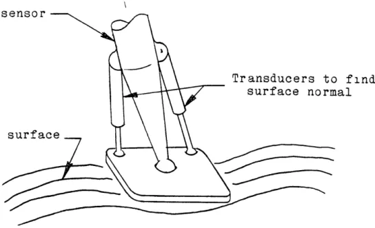
read a surface normal, see Fig 4 1 Adding more degrees of freedom significantly increases mechanical complexity,

the amount of data that must be transmitted to the computer, and computation time There is another problem in that the surface normal would be oe found for only one small spot The surface normal in the immediate neighborhood of the point would only be implied The average surface normal over a larger area could be found but would be at the expense of resolution of the point location The surface normal could be found more accuratly if the points touched were densely packed, but then the points themselves describe the surface normal

Although the ability to sense the direction of the surface normal would increase the surface description capabilities of a touch sensor, it was decided that it was not worth adding two more degrees of freedom Since three adjacent surface points describe an average surface normal, it was felt there was no need to find it for every single point

It was found to oe useful, though, to record the touch sensor direction for each point This was actually the center line of the touch sensor at the instant a point was touched The touch direction was easily found oecause it nad to be known to calculate the coordinates of the point anyway The touch direction was useful because it defined a line that could not pass through the surface This helped to define inside from outside A series of points on a plane can descrioe a surface normal out cannot, by

themselves, describe which side of the plane is tne outer side

4 1 2 Rigid or Flexible Base

A touch sensor mounted rigidly to the manipulator would be more reiiable and accurate than one mounted on a flexible base The mathematics required to find its coordinates would be simpler and so would its mechanical complexity It might seem that a rigid mounted sensor would be the best But there are some advantages to a flexibly mounted sensor

that may outweigh its disadvantages One advantage of a flexibly mounted sensor is that the manipulator would not have to come to a complete stop when a point was touched Tne sensor could just bend out of the way and not impede the continuous motion of the manipulator This would allow faster motion of the manipulator and would reduce tne risk of damage to the manipulator, sensor, or the object to oe touched Another advantage would oe that many sensors could be used at once if they were all on flexible mounts When one sensor nit a surface, it could respond and then bend out of the way to let the next sensor touch, see Fig 4 2

Flexible-base touch sensors could be constructed with or without degrees of freedom The type witnout degrees of

freedom would only work when straight, then simply shut off when bent over so as not to register any erroneous points

find Lal

surface

Touch Sensor with Surface Normal Touch Sensing Capability

Tip switch

on-point recorded Tip switch

on-point not recorded

Fig 4 2 Flexible Base Touch Sensor Fig 4 1

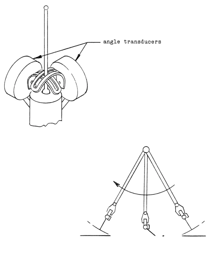
still register points even when bent over, see Fig 4 3

This way, a continuous stream of points could be read in one motion The trade off would come when deciding whether it is more important to have fewer degrees of freedom or the capability to read many points with one sensor

4 1 3 Where to Mount the Sensor

Since the sensor is to work with a manipulator, the most likely place to mount the sensor would be on the manipulator itself If the sensor were mounted at the wrist of the manipulator, the sensor would have six degrees of freedom and be most maneuverable If it were too awkward to use the wrist, the next oest mount would be the forearm of the manipulator This would reduce the number of calculations required to locate the sensor in space but would still leave three degrees of freedom

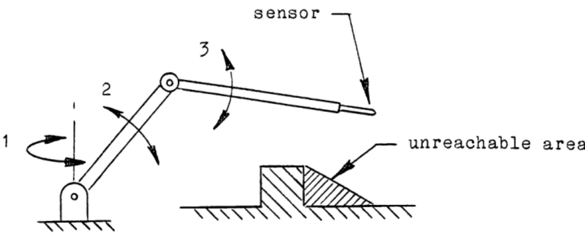
The sensor could theoreticly reacn any point in front of the manipulator but the sensor would only be able to approach any one point from one direction The sensor would not be able to reach around an object in the way, see Fig 4 4 A solution might be to install many sensors on the arm

protruding in all different directions so as to oe able to reach all points with at least one sensor, see Fig 4 5

The very best mounting location woald be to have tne sensor mounted on its own arm This could run completely independent of the manipulator and be controlled by a

angle transducers

Fig 4 3 Touch Sensor with Extra Two Degrees of Freedom A long string of points could be recorded with one

- unreachable area

Fig _{4 4 3 Degree of Freedom Manipulator with Interference} Problem

Fig 4 5 Solution to Interference Problem

Several mounted touch sensors could reach more areas and would not increase the degrees of freedom of the manipulator

different operator or perhaps be completely controlled by computer A computer could be programmed to randomly sweep the sensor around and to concentrate on relatively untouched areas

4 2 Touch Sensors Used in Experiments

The touch sensors that were built for experiments were designed solely to get surface points into the computer as efficiently as possible The touch sensors jere always mounted firmly in the jaws of the manipulator and only on-off electrical switches were used to send signals to the computer

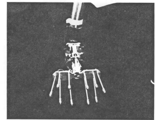
The first sensor built had 10 switches on it and each was connected seperately to digital inputs on the analog to digital converter, see Fig 4 6 The switches were mounted on somewhat flexible stems and were arranged like a brush It was found tnat a shorter stem provided the most accurate point coordinates and a slight convex curve to tne profile of the endpoints of the stems allowed the sensor to be rociked across a surface to collect a maximum amount of points

This brush sensor had some proolems that made it difficult to use The biggest problem was that tne switches worked only when pressed from one direction When a svitch was hit from the side nothing woald happen This meant the sensors always nad to oe pointed in the direction the

manipulator was being moved to makie sure tne switches would be hit straight-on Another problem was the sensors were too far from the base of the manipulator wrist It turned out that the joint angles of the wrist could not be calculated accuratly and errors multiplied the farther the sensors were from the base of the wrist

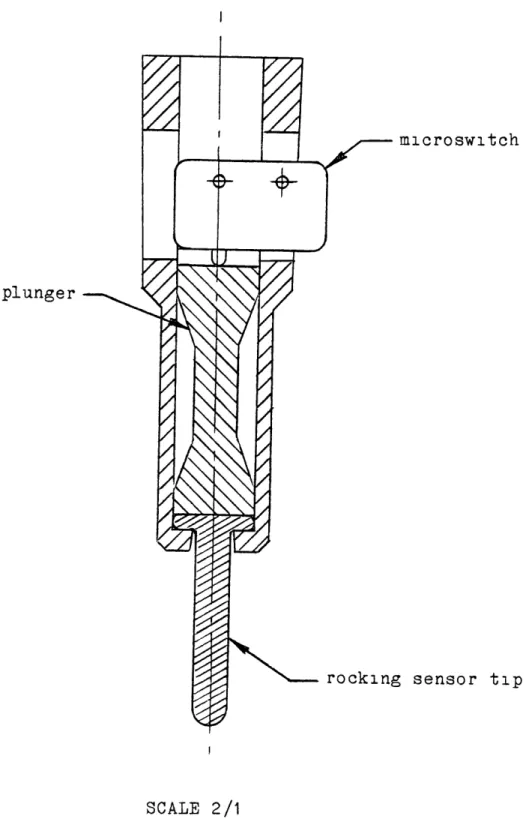
The second sensor built nad only one switch on it, see Fig 4 7 This was oecause in later experiments it was desirable to be able to select Individual points on a surface Also, the second touch sensor das located suca that one degree of freedom of the wrist was not needed to calculate the sensor's coordinates

Although the brush sensor had many more switches on it, the second sensor could collect points just about as fast This was because the second sensor was made to be sensitive when approaching a surface from any direction, see Fig 4 8 Besides being easier to maneuver tnan the brush sensor

it could also be moved faster because the manipulator only had to move at the wrist to trigger the switch The brush sensor required that the entire manipulator be moved to get the switches to approach the surface from the correct direction

Fig. 4.6: Brush Touch Sensor

microswitch

g sensor tip

SCALE 2/1

Fig 4 8 Switch Mechanism that is Sensitive to Touch from All Angles

CALCULATION OF POINT COORDINATES

5 1 Description

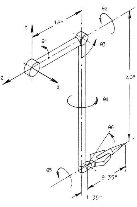
The picture of the manipulator was refreshed about every 20 milliseconds while the touch sensor program was running To do this, the new angles of tne maniplator had to be read every cycle The coordinates of a touch point would be calculated during the cycle also whenever a touch sensor was activated This was done by computing tne sequential angular transformations from the oase of the manipulator to the touch sensor tip Intermediate transformations from each manipulator link were saved so the manipulator itself could oe drawn on the graphic display

The coordinates of touch points were calculated and stored using the manipulator base as a relative origin and the x, y, and z axes were as shown in Fig 5 1 Only integer

values could be sent to the display processor so length units were cnosen such that there were 40 units per inch These units were chosen to minimize round off error and at the same time not overrun the display processor maximum length values, (plus or minas 2048) The basis for the dynamic display of this manipulator was developed by C Winey and is explained in some detail in Ref [1]

5 2 Proolems with the Manipulator

The manipulator that was used to maneuver tne touch CHAPTER 5

18" I

Fig 5 1 Manipulator Coordinate System 18"\

-I.

sensor was built to be controlled by a numan who would have direct visual feedback as to where he was moving it This type of control system did not require accurate positioning because it was assumed the operator would compensate for errors Consequently the manipulator was not very good for finding absolute point locations This posed some unique

proolems to getting accurate point angles The proolem could oe rectified by using a more rigid manipulator with less elasticity and "free play"

5 2 1 Cables and Gears

The joints of the manipulator were connected to the servos and position transducers by a series of cables and gears This allowed for much backlash and flexibility which translated into errors for recorded joint angles Any error in joint angles in turn translated into larger errors in calculated point coordinates One way tqese errors were minimized was to make the touch sensor sensitive to very light pressure to reduce the strain on the caoles Another solution was to minimize tne effect joint angle errors had on point coordinates The wrist joints were most prone to errors because they were connected with the longest cables Their effect was minimized by keeping the toucn sensor as close to the base of the wrist as possiole

5 2 2 Pushrod

The elbow joint of the manipulator was connected to its servo and transducer by the pushrod arraingement shown in Fig 5 2 At first it was thought that tne gear angle Ag would respond very much the same as the elbow angle Ae and that they could be considered as equivalent For relative motions this worked well enough but for calculating absolute point locations, the long forearm length multiplied a small angle error into a large position error Fig 5 3a shows the calculated locations of points on a flat square grid when it was assumed that Ag and A3 were the same Clearly

this assumption Is invalid for absolute positioning

An equation had to be developed to calculate the elbow joint angle A3 from the two angles it was dependent on, Ag and the X motion angle A2 A closed solution for A3 would oe very long because the linkage was 3-dimensional and relatively complex This was to be avoided if tie calculations were to be done in real-time Since the angle A3 was to be calculated for small incremental cnanges on each cycle it was decided to use the previous value of A3 on some preliminary calculations when figuring the new A3 Guessing the new value of A3 could eliminate some long calculations that really did not nave much effect on the final answer The metnod used was to calculate the x, y, and z locations at each end of the pushrod using Eq 5 1

A3

-Ag

(in Z,Y plane)

(Xg, Yg, Zg) (in X,Y plane)

Fig 5 2 Nonlinear Pushrod

Dn

, Ze)

(5 1 )

a ) Xg =3 10

b ) Yg =-4 5 sin( Ag )

c )

Zg =4 5 cos( Ag )

d ) X3 = 2 25 cos( A2 )- 4 5 sin( A2 ) cos( A3 ) e ) Y3 = 18 + 4 5 sin( A3 )

f ) Z3 = 2 25 sin( A2 ) + 4 5 cos( A2 ) cos( A3 )

The pusnrod length was known to be 18 02 inches and could also be defined in Eq 5 2

( 5 2 ) 18 02 = (X3 - g)2 + (Y3 - (Z3 -Zg

Between Equations 5 1 and 5 2 there are 7 equations and 9 variables The two variables A2 and Ag are known so all the others should be defined if the equations are all linearly independent The problem is that A3 appears 3

times, once in a sine function in Eq 5 le and twice in a cosine funtion in Eqs 5 id and 5 if This makes tne problem of calculating A3 very nonlinear and makes it useful to do some guessing If it is assumed tqat A3 is usually near zero, tnen small errors in A3 will have little effect on cos(A3) That means it should not make much difference If the value of A3 from the previous cycle is used to

calculate cos(A3) in Eqs 5 Id and 5 if If this is done then it is a straignt foward problem to calculate tne neq value of A3 from Eq 5 le Equation 5 2 can be converted to

( 5 3 ) Y3 = Yg +V18 022 - (X3 - Xg) - (Z3 - Zg)'

And from Equation 5 le ,

( 5 4 ) A3 = arcsin(( Y3 - 18 )/4 5)

This method of calculating A3 worked very well even when the angle of A3 went up to 60 degrees A value of A3 was converged upon fast enough that only one iteration per cycle was required Figure 5 3b shows how points iere located on a square grid with the angle A3 computed with tne above routine

Fig. 5.3a: Grid Errors Due to Pushrod Nonlinearity

POLYHEDRA CONSTRUCTION

6 1 Introduction

The previous chapter described a method of finding 3-dimensional point locations on a surface It oecame apparent later that it would be very useful to have a way of describing the surface the points where found on To have a geometric description of the surface would make it feasible to delete hidden lines and surfaces because a definite edge would be defined It would also provide a basis for deciding inside from outside and make it possible to calculate volume and surface area

First, simply connecting each point to its three nearest neighbors on the graphic display was tried This had disappointing results because the lines tended to

cluster in small bunches and didn't interconnect very much The approach was discarded because it didn't give any

semblance of a closed object and was no better than bare dots for making a recognizable picture

It is a trivial problem for human to connect a given set of points with lines to make a closed shape so it would seem that a solution solvaole by a computer aould be possible The problem is a human can make a judgement based on the whole set of points at once while a computer can only operate on a very small portion at a time This means an

iterative process must be found to construct the surface

with the aid of a computer

It was decided to treat tne surface as a geometric polyhedron (this is what tne surface would come out as anyway if the surface is constucted properly) Also, a constraint was imposed that the polyhedron surface be made up entirely of triangular facets This was done because it provides the computer the simplest possible surface segments to process Also, triangular facets give the greatest resolution for a given number of points A four sided facet connecting four dots would be the same as two triangular facets without the cross line

6 2 2-Dimensional Solution

The 2-dimensional solution to the problem will be shown first because it has many analogies to tne 3-dimensional solution but is mucn easier to explain In this case there are points scattered randomly on the edges of a flat area in two-space The problem consists of finding the best way of connecting the points to enclose the area and describe its edge, see Fig 6 1

The problem is fairly trivial if tne area in question is completely convex The correct way to connect any combination of edge points will always come out a convex polygon and any wrong solution will have some lines tnat cross over one anotner This suggests an algorithm where a computer could try every possible line connection

combination until it came across a solution where tnere were no crossing lines The trouble is that tne number of

required trials would go up exponentially with the number of points to connect

The solution to this problem that is most similar to tne one used to solve the 3-D problem is an iterative approach First, any 3 points are connected with lines to form a triangle Now if the area is still convex then all the other points lie outside this triangle

It is Important at this stage to define inside from outside for eacn line because the computer will only consider one line at a time It can be seen from Fig 6 2 that the three lines of the triangle can be defined as 1-2, 2-3, and 3-1 assuming that the x-y locations of points 1, 2, and 3 are known The line 1-2 can be thought of as a vector with base 1 and end 2 Now the outer side this vector can be defined arbitrarily as its right side

After the initial triangle is made and inside and outside defined, it is a straightfoward problem to add each point onto tne existing polygon An example is shown in Fig 6 2 Point 4 is to be added to polygon 1-2, 2-3, 3-1 It is apparent that line 1-2 is the only one that faces out toward point 4, (there will always be just one such line if the area is convex) Jow the line 1-2 can be deleted and the lines 1-4 and 4-2 added to make a new polygon 1-4, 4-2, 2-3, 3-1 Tne only decisive +ask for tqe computer is to

Area to be examined

Fig 6 1 _{Connecting 2-D Surface Points into Polygon}

2

1-2 "' 0 4

sequence specifles point connection

and outer side of each line

Fig 6 2 Definition of Lines and Polygons

f---sur ace points

scribin

ol on

find the line whicn is best to attach the point

The problem becomes more complex if areas with concave edges are allowed Many different polygons can be made from a given set of points if there are concave edges, see Fig

6 3 What can be done to limit the number of possible polygons to one9

If it can be assumed that touch sensors were used to find the points, then data about the direction from which the point was approached will be available A "touch vector" can be associated witn each point to indicate its outer side, see Fig 6 4 Note that the touch vector does not necessarily have to be at right angles to the edge touched It is only the centerline of the touch sensor at the instant the point is touched Now a single polygon solution is again possible if the constraint is imposed tnat the touch vectors cannot pass through the polygon, see Fig 6 5 Also, for computer control, there will only be one

line on the polygon available to attach a new point to, (if any) If tne new point is found to be inside tne existing polygon then tne correct line to attacn it to is tqe one tne touch vector passes through

Some proolems can occur with convex polygons It is

possiole to come across a point that qas no line on the polygon that it can attach to without violating a rule, see Fig 6 6a In these situations, the point must be thrown out or set aside until tne poljgon is developed enough to

wrong solution

Fig 6 3 Concave Polygons

In general, there are many ways to connect points found on a concave area and still get a closed polygon

. . . . .- - . .. . -t . . . L

0 UUU I

are:

Fig 6 4 Definition _{of Touch Vectors}

right solution

touch vectors must always point away from the polygon

Fig 6 5 Constructing Concave Polygons with Touch Vectors There will only be one polygon solution if touch vectors are considered

accept the point Another problem witn convex areas is that a folded polygon can be constructed by the computer, see Fig 6 6b The solution to tnls problem is to ignore any point that has a touch vector that goes through any line on the polynedron from its outer side

It is also possible to attach a new point to a completely erroneous line if a finite lengta touch sensor is used on an extremely convoluted polygon, see Fig 6 7 This problem could be solved by putting a oend in the touch vector to more accurately simulate the touch sensor and its arm An easier solution is to ignore points found to be over a certain depth inside the polygon

6 3 3-Dimensional Solution

The problem here is to find a way to connect 3-D surface points with lines to make a polyhedron that closely resembles tne surface the on which points were found It turned out that the best way to solve the problem was not by analyzing tne connecting lines but by analyzing the facets of tqe polyhedron If the facets on a set of points is known then the edges are also known Triangular facets were

used as stated earlier

6 3 1 Polyhedron Description

A method is required to store the facets in computer memory It was decided to descrioe the facets as a sequence

1

2

a Point 6 cannot be attached to the existing polygon without causing a touch vector to pierce through It is not likely that point 6 Is even from the same area as points 1 - 5

b Point 6 cannot be attached to the polygon without turning it inside-out Point 6 will have to be ignored or saved until the polygon is further developed

nection lines

Int to be attached

touch vector

Fig 6 7 Example of an Incorrectly Attached Point

To keep the touch vector on the outside of the polyhedron, the touch point will have to attach to the wrong line This problem stems from the fact that touch vectors are considered to be infinitly long while the actual touch sensor is very short _{The simplest solution to this problem is to ignore or} save points tnat are found to be deeper in into the polyhedron than the length of the touch sensor

L ___~~

nncf%

lI

of points, because the points and their coordinates would be already known The facet 1-2-3 would be a facet witn edges connecting the points 1 to 2, 2 to 3, and 3 to 1 Also tne inside and outside of the facet could be defined with tnis number sequence using the right-hand-rule, see Fig 6 8 It can be seen that the facets 1-2-3, 3-1-2, and 2-3-1 all describe the same facet because the sequence always goes in the same direction around the triangle The facets 3-2-1, 2-1-3, and 1-3-2 describe the same facet as above but with the opposite outside surface

The computer description of a tetrahedron is shown in Fig 6 9 Note that each line on a polyhedron is given twice in the facet data, once on two different facets and always in opposite sequence It might seem easier to describe the polyhedron bj s+oring the lines as two-number sequences rather than the apparently redundant method of storing facets as three-number sequences But it turns out to be very Important to know the complete facets and this data would not be readily avallaole with line information

Like the 2-D solution, restraints were imposed that restricted the configuration of the polyhedron No surfaces were allowed to stick through one another and no touch vector could be allowed to exist on the inside of the polyhedron Also, 11Ke the 2-D solution, an iterative approach was used where each point was added onto an

2

outer side of surface

Facet 1 - 2 - 3

Fig 6 8 3-D Definition of Facets

Number sequence defines point connection and outer side of facet using the right-hand-rule

1 Polyhedron described by facet data 1-2-3 1 -3-4 4-2-1 3-2-4

How can a new point be added onto a polyhedron9 _First,

it is helpfull to exploit some of the useful properties of polyhedrons as described by Euler's formula for polyhedrons, where F is the number of faces on a polyhedron, E is the

number of edges or connecting lines, and V is the number of vertices or points

( 6 1

)

F =

E -

V +2

This equation holds for any ordinary 3-D polyhedron that does not have any holes passing through it

Only polyhedrons with triangular facets will be considered so another defining equation is given On a polynedron with triangular facets it can be seen that each facet has exactly 3 edges and that each edge seperates exactly two facets Thus

( 6 2 ) 3F = 2E (for triangle faceted poljhedrons) Combining Eqs 6 1 and 6 2 gives two relations

(63)

F =2V-4

(6 4)

E = 3V - 6

Equations 6 3 and 6 4 show that for each new point added to a triangular polynedron there will have to be 2 more facets and 3 more lines

For the 2-D solution a point was added onto tne existing polygon by deleting one chosen line and adding 2 more In effect, the point was attached to the place were one line used to be In the 3-D solution a facet must be chosen on the e-isting polyhedron on which attach the new

point That facet is then deleted and tne resulting hole is closed by adding 3 new adjacent facets that reached out to the new point, see Fig 6 10 Tnis procedure satisfies

Equation 6 3, in the total number of facets added to tre polyhedron for eacn new point It is also apparent from Fig 6 10 that Equation 6 4 is satisfied because exactly 3

new lines are added

One of biggest proolems was deciding which facet to attach the point to Unlike the 2-D problem there was not always a single answer, even when touch vectors were considered In general there could be several facets that a point could be attached to that would produce a closed polyhedron and would not cause any touch vectors to stick through any surface More restraints had to be incorporated to make the computer converge on a single facet

One restraint added to the program was that if a facet was pierced from the negative side of the touch vector of a new point, then that point must attach to tnat facet, assuming all the other restraints are satisfied This restraint worked very well in situations where the new point was close to the polyhedron and the touch vector most likely

passed through the best facet

Sometimes, though, the new point was so far away that its touch vector did not pass through the polyhedron at all and if it did, the facet it pierced through was not likely to oe the oest To cover tqese situations a secondary

5

a. Point 6 shown with chosen facet for attachment

S 7i

b. Completed attachment

restraint was added which required tqat the new point attach to the facet with the nearest centroid

If the new point was very far away from the polyhedron, there would be very little chance the new point would attach to a good facet, see Fig 6 11 The solution to this problem was to ignore points over a specified distance away Taken together, these restraints caused the computer to

converge on a single facet and usually it was the oest one Even when the chosen facet did not look like tne best, the next step of processing usually converged on a better

solution for the polyhedron

Many times the new point was found to be on the inside of the polyhedron In these cases there was at least one facet that could be found which the point's touch vector pierced from the inside This was tne only facet the interior point could attach to and keep its touch vector on the outside of the polyhedron, see Fig 6 12

6 3 2 Initializing the Polyhedron

The above procedure worked only at adding points to an existing polyhedron A seperate algorithim was required to create a starting polyhedron from a set of initially unconnected points The method used only -equired 3 points to make an imaginary two sided polyhedron The computer was simply Instructed tnat there were two facets, one on each sde of zne triangle defiqed by tqe 3 new points, see Fig

Fig 6 11 Possible Errors from Attachment of Distant Points In general, it is very difficult to make a rational decision on whicn facet to attach a distant point to The choice, tnough, can nave a drastic effect on the resulting shape of the polyhedron The easiest solution to this problem is to ignore points that are over a certain distance from the

,ctor

,elow nolvhedron surface

Fig 6 12 Attachement of Interior Points

Interior points must always attach to the facet that the touch vector pierces through

1

initialization facets 1-2-3

3-2-1

Fig 6 13 Initialization of Polyhedron

First 3 points are connected with 2 facets to make psuedo-closed polyhedron

6 13 The computer had no capacity to reject sucn an Impossible polyhedron once it had been installed Any 3 noncolinear points in space can be connected this way and will not technically violate any of the stated polyhedron rules This entity also satisfied Equations 6 3 and 6 4 which specify the correct number of verticies, edges, and faces for a real polyhedron

When the 4th point is added on, the computer ll use the usual algorithm to erase one of the coplaner facets and add 3 more to make a tetrahedron The reason that a tetrahedron was not used for initialization is tnat too much programing space would be required make sure the shape was not inside out and also that none of the touch vectors where piercing through

6 3 3 Cnecking Facet Pairs

After a new point had been attacned to the polyhedron, the facets were not usually in the best configuration The new point could be sitting on the top of a long spike or otherwise looking as though it was stuck on as an

afterthought, see Fig 6 14

Since there were usually many possiole polyhedron configurations that a given set of points could be built into, some new critera had to be used to make sure that one polyhedron solution was decided upon

a. New point attached to polyhedron without smoothing.

q

b. After smoothing.

Fig. 6.14: Need for Smoothing of Polyhedron

adjacent pairs of facets and, if required, replace them with compliment facets Figure 6 15 shows how the four corner points connected by any two adjacent triangles could also be the corner points of two otner completely different triangles The facets 8-6-5 and 5-6-7 are the starting facets and 8-6-7 and 8-7-5 are tne compliment facets An entire polyhedron could be modified bit by bit by changing facet pairs and the polyhedron would never have to oe considered as a whole

The primary criterion used for deciding if a pair of facets should changed was based on the idea that a polyhedron with the smoothest surface will be the best In other words a polyhedron would be seached for that had a minimum average angle oetween facets This was done by comparing the pair of facets, considered for changing, to their four neighboring facets The algorithm checked tae

angular difference between 1) the original facets 2) the compliment facets

3) the neighboring facets and the pair to oe checked 4) the neighooring facets with the compliment facets

This gave 5 angular differences to average for each of two polynedron surfaces If tqe complimentary facet arrangement was found to have less average angular difference, then the facets would oe changed

Facet Pair 8-6-5, 5-6-7

Compliment Facet Pair 8-6-7, 8-7-5

to change a pair of facets New facets could not be allowed to stick through another surface of the polyhedron Al41so, a check had to be made that none of the touch vectors of the points on the polyhedron pierced through the new facets The change in facets would be stopped if any of the above happened

It was possible to come across a pair of facets tnat had no reasonable compliment These facet pairs were not considered changable and were found by checking to see if any of the compliment cross-lines were already occupied by other facets

It would not be expected to find a touch vector that lay at an angle of greater than 90 degrees to tne surface normal of an adjacent polyhedron facet The computer, though, would construct a polynedron this way if not

instructed to consider touch vector angles Therefore, anotner restraint was added that any facet pair had to be made convex if it had a corner point with a toucn vector that pointed away from its surface normal at greater than 90 degrees

The above requirements nad to have certain priorities because tney very often conflicted witn one another Tqe

order of priority was

1) The polyhedron must remain a closed ooject and cannot be allowed to fold on itself or wrap inside out Also all touch vectors must exist on the outside of the

polynedron and cannot be allowed to stick through

2) Any facet pai- dith a touch vector that pointed away at greater than 90 degrees from its surface normal had to oe convex

3) The facet pair that had the least average difference between themselves and tneir four neignbors nad to be cnosen

When one pair of facets were converted, it affected all the neighboring facets as to whether they still followed the above requirements This meant all these facets had to be rechecked

The routine used to decide which facets to check das fairly simple First all the facets were cnecked around tne spot where a new touch point was added to the polyhedron Then, if one of these facets was converted, all its neighboring facets were put in a list of facets to be

cnecked The routine stopped when the list das empty Sometimes a pair of facets to oe changed could get skipped over because the list ias limited to 30 points These facets would be found by using an operator controlled option that cnecked every facet pair on the polyhedron to catch any that were incorrect

There was some concern tqat a polyhedron might be formed that would have a cnain of mutually dependent facet pairs In otner words eacn facet change 4ould cause tne neighboring facets to change and an endless loop of changing

facets would be formed The existence of such a polyhedron has not been proven but it das never observed to occur The computer program would always converge on a polyhedron where all the facet pairs satisfied the requirements

6 3 4 Quality of the Polyhedron Shapes

It might seem that there would always be one solution that the computer would converge upon This was not always true Sometimes the polyhedron would get into a oad shape the computer algorithm could not get it out of This due to the fact tnat the computer algorithim based its decisions on only one pair of facets at a time There was no way for the computer to get to better facet configuration if the first facet change meant putting tne polyhedron in an impossible shape

The method used to keep the polyhedron from locking into bad shapes was to make sure that new points were not added an unreasonaole distance away from the existing polyhedron If the maximum distance was held to witnin the general feature dimensions of the object being touched then the points would attacn onto reasonable areas It would be very difficult to attach a new point to a developed polyhedron in tne right place if tne polyhedron was roughly one foot across and the new point was more than two feet away, see Fig 6 12

METHODS OF DISPLAY

7 1 Introduction

The 3-dimensional information needed to completely describe points and polynedrons in space can be easily stored as data in a computer But if these data are just displayed as lists of numbers, it w11 be absolutely meaningless to a human A grapnic display can show 3-dimensional data much better but suffers from the fact

that it can only display a 2-dimensional picture This chapter will consider different methods of bringing out 3-dimensionality for data to be shown on a grapanc display

7 2 Problems with Polyhedra Displays

Most of the methods used to display 3-dimensionality descrioed here were developed long before it was possible to create polyhedra from point data It would have oeen very difficult to understand what was nappening in the program witnout it This was because it was impossible to tell what the computer was constructing in 3-D, without a good metnod of viewing it A polyhedron drawn on a vector grapnic displaj just looked like a mass of connected lines if hidden segments were not removed There was no way to tell If one triangle was sticking tnough another triangle in 3-space when only one flat view was available, see Fig 7 1

There are several ways to improve the depth ot a flat CHAPTER 7

a) Potogaphb) Points Only

c) Polyhedron d) Polyhedron with Contours

Fig. 7.1 Different Displays for One Set of Facets · · _·· ~_{· · ·}

·

picture Showing perspective is one way out it is best suited to rectangular shapes Triangles shown in perspective just look like slightly different triangles Deleting hidden lines and providing shading are methods that bring out depth for a numan but can be very slow to process in real time A metnod using raster graphics to remove hidden surfaces will be shown later in this chapter but was only good at getting a static picture C Winey [ 1 ] did

studies on showing two orthogonal pictures on the screen at once and displaying a shadow to help define 3-dimensionality These methods worked well for displays where related features could be distinguished in each view and were used successfully for maneuvering the touch sensor on the screen It was difficult, though, to distinguish related points on a complex polyhedron shown in dual views

7 3 1 Rotating the Picture

It was found that rotating the polyhedron on the screen helped to bring out its 3-dimensionality Features in the back of the picture moved one way and features in front of the picture moved the other way Specific details could be seen also if the p cture was rotated a full 360 degrees For example, it could be seen whether or not a line was

plercing a triangle if the picture was turned completelj around If a line was not piercing a facet, then there has to oe at least one place in the rotations on tne screen

where the line does not lay across the facet

To give the appearance of a rotating picture, the object coordinates were calculated for a small Incremental angle change and the picture was redrawn on the display It was possible to redraw the picture rapidly enough to give the illusion of smooth rotation The object could be viewed from any angle if it was first rotated about an axis This could be done by multiplying the X, Y, and Z coordinates of the object by a rotation matrix [ T ] to get the new coordinates X', Y', and Z'

[ x', Y', Z',

1

i

=

[

K,

Y, Z,

1 0 0

[ T ] = 0 cos(A) -sin(A)

0 sin(A) cos(A)

0 0 0

( for rotation around the

cos(A) 0 sin(A)

[T = 0 1 0

-sin(4) O cos(A)

0

0

0

( for rotation around the cos(A) -sin(A) 0

[

T

sin(A)

cos(A

0

0

0

1

S

( for rotation around the

1

Il

T

i

T

0

0

0

1

x axis

)

O

0

0

y axis

)

0

0

0

1

z axis

)

The orientations of the display coordinates and tne (7 1

where

(72

(73)

Fig 7 2a A positive rotation is defined as counter-clockwise ghen looking down that rotation axis

Since the display consisted of points in space either connected or disconnected, all that was required to be transformed was the coordinates of the points The "connectivity" would not change no matter what the angle of view

A combination of rotations could be made by multiplying the rotation matrices together The equation,

( 7 5 ) [ T ] = [ Tz ][ Ty ][ Tx ]

is equivalent to a rotation around the z axis, then around the y axis, and then around the x axis It is important to keep the order of multiplication straignt or different views will result

It is convenient to describe all the terms of the transformation matlx as shown in Equation 7 6

(76)

XX YX ZX O0 [T]= XY YY ZY 0

XZ YZ ZZ O

LXT

YT ZT

1

The terms XX thru ZZ handle rotations and their values are usually determined by equations 7 2, 7 3, and 7 4 TX, TY, and TZ are translational values that define the position of the object relative to its own coordinate system These are important if it is desi-ed to zoom in on a small section of the object A zoom effect is possible by multipling all

terms of the transformation matrix by a size factor

The Megatek Display Processor had the capability to do rotations in hardware The 3 coordinates of all the points defining the features of tne object were first stored in Megatek memory Then it was given the required rotation

terms and the Megatek would take care of calculating the transformations for each point This saved having to do the calculations for each point in software and also reduced the amount of data that had to be sent to the Hlegatek Very fast and smooth rotations were possible regardless of tne complexity of the display The transformation terms required by the Megatek were XX, XY, XZ, XT, YX, YY, YZ, and YT The rest of the terms only affect the z plane of the

display which cannot be seen on a 2-D screen

The Megatek rotations always occured around the origin of the object as it was installed in display memory This was inconvenient because very often a small portion of the display would be zoomed in on and would also need to be rotated With the object rotating about its center the small portion would generally rotate rignt out of view The cure for this was to cause tne object to always rotate around in screen origin The XT and YT terms sent to tne Megatek affected the x-y posilions of points in screen coordinates Tnese terms could be altered each time the picture was rotated to keep tne object on screen center To do tals, the translations in object coordinates nad to be

specified, (Xo, Yo, Zo) This was done by manuvering tqe desired rotational base to the center of tne screen by viewing two orthogonal views Now the picture would always rotate about that base if XT and YT were recalculated every iteration by the equations,

( 7 7 ) XT = XoXX + YoXY + ZoXZ ( 7 8 ) YT = XoYX + YoYY + ZoYZ

XX, XY, XZ, YX, YY, and YZ had to be calculated first for

that rotation

There is a problem with dynamic pictures that are rotated with the above transformations There will be no

Indication which is front and which is bacK on an object when no hidden lines are removed and no perspective is shown kn object can be rotating on the screen and some people viewing it will say its rotating to the left while others say its rotating to the right The mind tends to lock on one rotation and can be difficult to change One way found to remedy the proolem was to memorize the correct rotation for each input but it was too easy to forget The most useful method was to have a known zero position the the picture could be put in, where front and back were enown Another solution might oe to have a coordinate indicator on tne screen consisting of writing Front and back are easily distinguished with writing because it cannot oe read when it is shown reversed