Complex materials handling and assembly systems.

COMPLEX MATERIALS HANDLING AND ASSEMBLY SYSTEMS Final Report

June 1, 1976 to July 31, 1978

Volume IX

ANALYSIS OF TRANSFER LINES CONSISTING OF THREE UNRELIABLE MACHINES AND TWO FINITE STORAGE BUFFERS

by

Stanley B. Gershwin Irvin C. Schick*

This research was carried out in the M.I.T. Electronic Systems Laboratory (now called the Laboratory for Information and Decision Systems) with support extended by National Science Foundation Grants NSF/RANN APR76-12036 and DAR78-17826.

Laboratory for Information and Decision Systems Massachusetts Institute of Technology

Cambridge, Mass. 02139

An important class of systems, which arises in manufacturing, chemical process, and computer contexts, is one where objects move sequentially from one work station to another, and where they rest between stations in buffers. In the manufacturing context, such systems are called transfer lines or

flow shops.

In the research reported here, the dynamic behavior of a buffered trans-fer line with unreliable work stations is modelled as a Markov chain. The system states are defined as the operational conditions of the stages and the levels of material in the storages. The steady-state probabilities of these states are sought in order to establish relationships between system parameters and performance measures such as production rate (efficiency), forced-down times, and expected in-process inventory.

The steady state probabilities are found by choosing a sum-of-products-form solution for a class of states, and deriving the remaining expressions by using the transition equations. In this way, the order of the system of

equations to be solved is drastically reduced. Various properties of this reduced-order system are discussed, as well as methods to improve its numerical behavior.

This algorithm suggests a general technique for solving large-scale, structured Markov chain problems.

In order for this volume to be self-contained, some material in Chapters 2 and 3 reproduce material that has already appeared in Volume VI of this report (Schick and Gershwin [1978]).

Thanks are due to Mr. Wei-Tek Tsai for his early help with the computer program and Fig. 4.1. Mr. Steven C. Glassman did an excellent job in writing the final version of the computer program, and he and Dr. Alan J. Laub and Ms. Virginia C. Klema provided useful advice on

the singular value decomposition method. Ms. Klema and Mr. John E. Ward also contributed editorial comments on the manuscript. Additional

analytical assistance and experience with the program was provided by Ms. Brenda Pomerance.

We thank Ms. Margaret Flaherty for typing the manuscript and Mr. Arthur J. Giordani and Mr. Norman Darling for drafting the figures.

We are most grateful to Dr. Bernard Chern of the National Science Foundation for his continuing sponsorship of our research in automated manufacturing and materials handling systems.

During the period June 1, 1976 to July 31, 1978, this research was supported by National Science Foundation Grant NSF/RANN APR76-12036.

Since August 1, 1978, it has been supported by National Science

Foundation Grant NSF/RANN DAR78-17826.

ABSTRACT ii

PREFACE iii

TABLE OF CONTENTS iv

LIST OF FIGURES vi

LIST OF TABLES vii

1. INTRODUCTION 1

1.1 Past Research 3

1.2 Overview of the Method 4

1.3 Outline of Report 5

2. MODELLING 6

2.1 The Unreliable Transfer Line with Interstage 6 Buffer Storages

2.2 State Space 7

2.3 Assumptions of the Model 8

2.4 The Markov Chain Model 9

2.5 General Results from Markov Chain Theory 15

2.6 Performance Measures 17

3. ANALYTICAL SOLUTION OF TRANSITION EQUATIONS 20

3.1 Internal State Transition Equations 20

3.2 The Sum-of-Products Solution for Internal State 22 Probabilities

3.3 Boundary State Expressions 26

3.3.1 Transient States 28

3.3.2 Boundary States Reachable from Internal States 31 in One Step

3.3.3 Other Expressions of Internal Form 33

3.3.4 Other Expressions 33

3.4 Reduction of the System of Equations 38

4. CONSTRUCTION OF THE PROBABILITY VECTOR 42

4.1 Analysis of the Parametric Equations 42

4.2 Analysis of the Reduced-Order System of Equations

4.3 Limiting Behavior of U 60

4.4 Limiting Behavior of i(u) 70

5. DISCUSSION OF METHOD AND RESULTS

75 5.1 Solution of Reduced-Order System: Memory

Requirements and Numerical Difficulties 5.2 Qualitative Discussions of the Solution

77 5.2.1 Magnitudes of i Expressions

79 5.2.2 Values of Uj, j = 1,..,

81 6. CONCLUSIONS AND AREAS OF FUTURE RESEARCH

6.1 Different Boundary Expressions 81

82 6.2 Choices of Uj, j= 1,...,

6.3 Alternative Models 84

APPENDIX

A. A SET OF BOUNDARY STATE TRANSITION EQUATIONS 85 97 B. (s., U) EXPRESSIONS WHICH ARE NON-ZERO AND NOT OF

INTERNAL FORM

C. LIMITING k (s) EXPRESSIONS 101

k 122

D. A COMPUTER PROGRAM FOR SOLVING THE THREE-STAGE 122 TRANSFER LINE PROBLEM, WITH SAMPLE OUTPUT

194 REFERENCE S

Figure 1.1: A k-stage transfer line 2

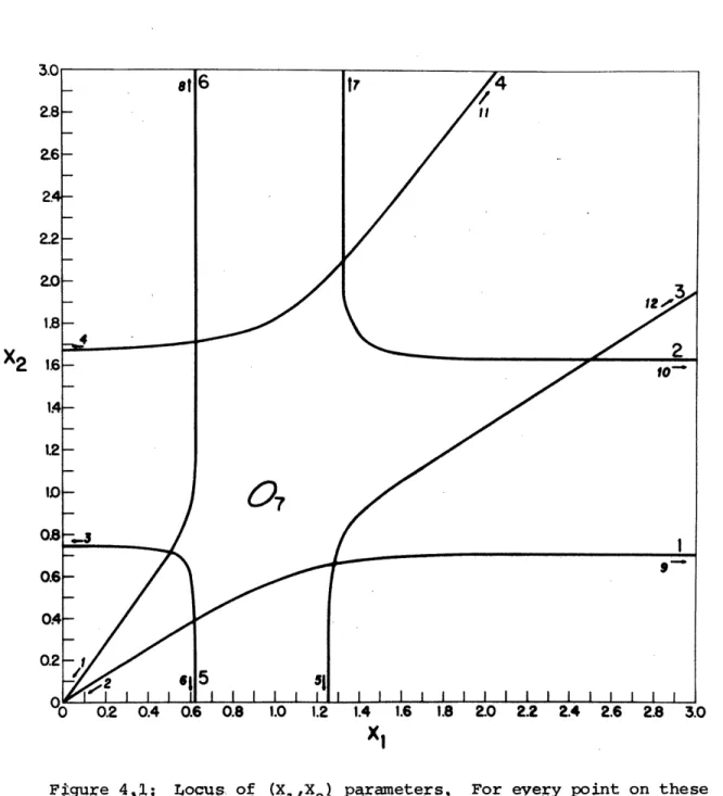
Figure 4.1: Locus of (X1 X 2) parameters 45

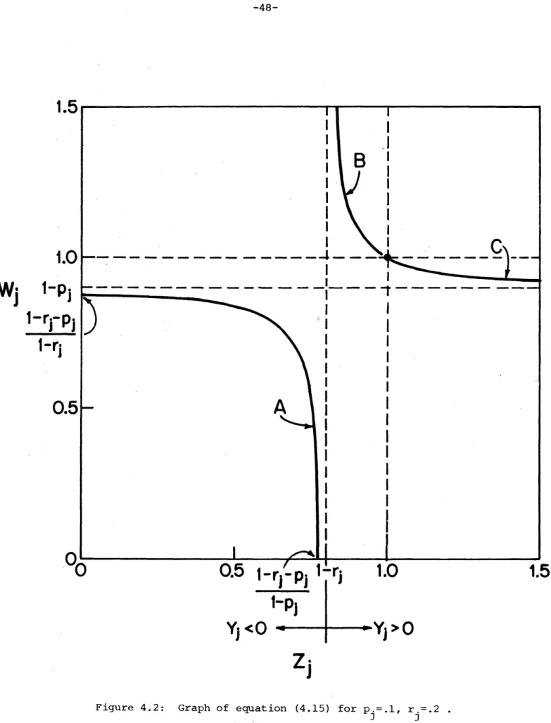
Figure 4.2: Graph of equation (4.15) 48

Figure 4.3: Non-zero k[s] regions 74

Table 2.1: Transition Probabilities for Machine Operating 11 Conditions

Table 2.2: Storage Level Transitions 12

Table 3.1: Transient States 29

Table 3.2: Boundary States Reachable from Internal States in 32 One Step

Table 3.3: Additional States of Internal Form 34

Table 3.4: Expressions Obtained in Pairs 36

Table 3.5: Expressions Obtained Singly 39

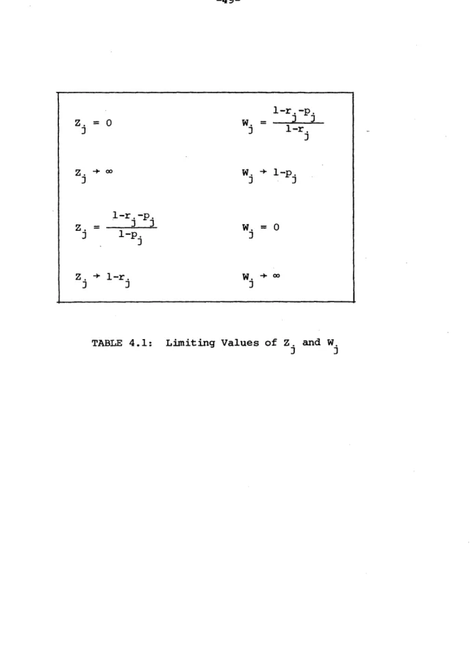
Table 4.1: Limiting Values of Z. and W. 49

J J

Table 4.2: Bounds on Sets A,B, and C 50

Table 4.3: Sign Combinations for the Curves on Figure 4.1 52

Table 4.4: Q, The Set of Odd States 55

Table 4.5: Limiting Qj Combinations 66

An important class of systems, which arises in manufacturing, chemi-cal process, and computer contexts-, is one where objects move sequentially

from one station to another, and where they rest between stations in buffers. In the manufacturing context, such systems are called transfer lines, and the stations are transfer machines. A schematic diagram of such a system appears in Figure 1.1,

In the research reported here, the dynamic behavior of a transfer line is modeled as a Markov chain, and a method is proposed for finding the steady state probability distribution of the states of that chain. The probability distribution is used to calculate such measures of per-formance as average efficiency (production rate) and average in-process

inventory. The method is applied here to three-stage systems. In a simpler form, the method has been applied to two-stage systems (Schick and Gershwin [1978], Gershwin and Berman [1978], Berman 119791). It

is hoped that the method presented here can be extended to longer lines and more complex networks.

In the model discussed in this report, the source of randomness is the unreliability of the workstations or machines. The machines fail at random times and remain inoperable for random periods during which they are under repair. It is possible to compensate for workstation failures by providing redundancy, i.e., secondary parallel stations that are brought into use in case of failures of primary machines. This process, however, can be prohibitively expensive if system components

are costly.

An alternative consists in placing buffer storages between unreliable stages. These provide temporary storage space for the products of

stations upstream of a failed station. Similarly, they provide temporary supplies of workpieces for stations downstream of a failed station.

Thus, they act so as to decrease the effects of workstation failures on the rest of the line.

However, costs of floor space, material handling equipment, and in-process inventory are also of great importance. It is thus necessary

-1-V - 0 o

F*

L

0)

_(D 0 9 + *-4 4 U CV)~~~~~() - 0) rjC L m - l- Cm

Io

m X C H *o

~~H

0

-

_{~~~~~~~~~~~~~~~~~-}

x.

0

H)

_V) 0)

~

- 10a C

to find in some predefined sense the "best" storage configuration; this

leads to an optimization problem. To solve this problem, it is essential

to be able to quantify the relations between transfer line design

para-meters (i.e. average up and down times of workstations, storage capacities)

and the performance measures.

1.1 Past Research

Transfer lines were first (Buzacott [1967a]) studied analytically

through a probabilistic

approach by Vladzievskii [11952]. Applications

of queueing networks and transfer line models are found in a wide range

of areas, including computer science, coal mining, the cotton, paper

and chemical industries, aircraft engine overhauling, and the automotive

and metal cutting industries; an extensive literature survey of related

work appears in Schick and Gershwin [1978].

The production rate of transfer lines in the absence of buffers

and in the presence of buffers of infinite capacity had been studied

by many researchers, including Buzacott [1967a, 1968], Hunt [1956],

Suzuki [1964], Rao [1975a], Avi-Itzhak and Yadin [1965], Morse [1965],

and Barlow and Proschan [1975].

Some authors analyze reliable transfer

lines where buffers are used to reduce the effects of fluctuations in

non-deterministic service times (Neuts [1968, 1970], Muth [1973],

Knott [1970a, 1970b], Hillier and Boling [1966], Hatcher [1969],

Patterson [1964]).

Unreliable two-stage systems with finite buffers have been studied

(Artamonov [1976], Gershwin [1973a], Gershwin and Schick [1977],

Gershwin and Berman [1978], Berman [1979], Buzacott [1967a, 1967b,

1969, 1972], Okamura and Yamashina [1977], Rao [1975a, 1975b],

Sevast'yanov [1962]).

Longer systems are more difficult to analyze

because of the complexity of machine interference when buffers are full

or empty (Okamura and Yamashina [1977]).

Such systems have been formulated in many ways (Gershwin and

Schick [1977], Sheskin [1974, 1976], Hildebrand [1968], Hatcher [1969],

Knott [1970a, 1970b],

Buzacott and Hanifin [1978]), and studied by

approximation (Buzacott [1967a, 1967b], Sevast'yanov [1962], Masso [1973], Masso and Smith [1974]), as well as simulation (Anderson [1968],

Anderson and Moodie [1969], Hanifin, Liberty and Taraman [1975], Hanifin, Buzacott and Taraman [1975], Barten [1962], Freeman [1964], Kay [1972], Ho, Eyler and Chien [1979]), but no analytic technique has been found to obtain the expected production rate of a multistage transfer line with unreliable components and finite interstage buffer storages. Schick

and Gershwin [1978] propose numerical, as well as analytical methods for solving this problem. This report completes the analytical solution proposed there.

1.2 Overview of the Method

To find the steady-state probability distribution of a Markov chain, it is necessary to solve a set of M linear transition equations in M unknowns, where M is the number of states of the chain. In the problem discussed here, M is large, so an efficient method is required.

This problem does have a structure that can be exploited. Due to that structure, it is possible to find Z vectors _j (j = 1,...,

i),

each of which satisfies M-k of the transition equations. Each of the Cj vectors fails to satisfy the same £ equations. Consequently if the probability vector is expressed as a linear combination of these vectors

p =

C'

(1.1)

j=l

'

then it is guaranteed to satisfy the M-2 equations each .j satisfies. In order to satisfy the remaining equations, the coefficients Cj must be appropriately chosen.

To do this requires solving R linear equations in Q unknowns. Since Z is much smaller than M, this is relatively easy to do.

The method is not without limitations. First, the k equations in the k unknowns C1, ..., CA are poorly behaved. It has been necessary

to use extended precision (32 decimal place) arithmetic to obtain 5 decimal place precision in analyzing transfer lines with large storages. Second, 2 increases with the storage sizes. Even though 2 increases

size of problem that can be treated. Also, this increase prevents the

method, as currently formulated, from being usefully applied to longer

lines. Effort is being devoted to overcoming these limitations.

1.3 Outline of Report

The problem is formally presented in Chapter 2. The transfer line

is described and the state space is formulated. The modelling assumptions

are stated, and a Markov chain model is introduced. Formulas for the

calculation of performance measures are derived.

Steady state transition equations are solved analytically in

Chapter 3. The equations involving only internal states are satisified

by a sum-of-products form for the steady-state probabilities.

Expres-sions are also obtained for the steady-state probabilities of boundary

states. The system of equations is then reduced in dimension.

The steady-state probability vector is derived in Chapter 4. The

sets of solutions of the four parametric equations in five unknowns are

analyzed and an efficient algorithm for computing solution points is

introduced. The reduced-order system of equations is studied and its

solution is discussed. The limiting behavior of probability

expres-sions as solutions of parametric equations approach limits is

investi-gated, towards rendering the system of equations better conditioned.

The reduced-order system of equations is solved, and shortcomings

of the algorithm, (memory requirements, numerical problems) are discussed

in Chapter 5. A qualitative discussion of the solution is given, and in

Chapter 6, tentative conclusionas pertaining to the method are presented.

A formal statement of the problem is given in this chapter. A multi-stage transfer line with unreliable components and intermulti-stage buffer storages is described in Section 2.1 and a state space formulation is introduced in Section 2.2.

The assumptions made in formulating the mathematical model are dis-cussed in Section 2.3. Most assumptions are standard. (See Buzacott and Shanthikumar [1978].)

A Markov chain model is introduced in Section 2.4 and the properties of such systems which are applicable to the present problem are discussed in Section 2.5. The performance measures are expressed as functions of state probabilities in Section 2.6.

2.1 The Unreliable Transfer Line with Interstage Buffer Storages The system under study consists of a linear network of servicing stations (machines) separated by finite capacity buffer storages (Figure 1.1). Workpieces enter the first machine from outside the system. Each

worpiece is processed by machine 1, after which it moves to storage 1.

The part moves in the downstream direction, from machine i to storage

i and on to machine i+l, until it is processed by the last station,

machine k, and leaves the system.

The specific nature of the machine operations is of no consequence

in the present analysis. In a metal working line, it may consist of

drilling or welding; in a computer network, the operation may be data

processing by a specific computing, storage, or input/output unit. It

is assumed, however, that the machines are synchronized. That is,

there is a common cycle time, and all machines that are operating on

pieces start at the same instant.

The buffer is a storage element. Parts pass through a buffer with

a transportation delay which is negligible compared to service times

in the machines, except for the delay caused by other parts in the queue.

Machines fail occasionally. Failures may have many causes and thus,

the down-times of failed machines, like the up-times of operating

machines, are random variables. When a failure occurs, the level in the

adjacent upstream storage tends to rise. If the failure persists long

-6-enough, that storage fills up and forces the machine upstream of it to

stop processing parts. Such a forced down machine is referred to as

blocked. Similarly, the level of the adjacent downstream storage tends

to fall during a failure, as the downstream machines continue to drain

its contents. If the failure persists long enough, the adjacent

down-stream storage empties and the machine downdown-stream of it stops processing

parts. Such a forced down machine is referred to as starved. These

effects propagate up and down the line if the repair is not made promptly.

By supplying workpieces, or room for workpieces to be put in,

inter-stage buffer storages partially decouple adjacent machines. While machine

failures are to some extent inevitable, the effects of a failure of one

of the machines on the operation of others is mitigated by the buffer

storages. When storages are empty or full, however, this decoupling

effect cannot take place. Thus, as the capacities of storages increase,

the probability of storages being empty or full decreases and the effects

of failures on the production rate of the system are reduced.

An inevitable consequence of buffers is in-process inventory. As

buffer capacities increase, more partially completed material is present

between processing stages.

The effects of interstage buffer storages on the transfer line

pro-duction rate and on the average in-process inventory are studied here

by formulating a state space description of the system and obtaining

the steady-state

probability

distribution,

2.2

State Space

It is natural to formulate the problem of calculating transfer line

performance parameters as one of analyzing a Markov chain. This is

because the probability of finding storages at a given level or machines

operational or under repair after a cycle depends on the storage level

and machine conditions before that cycle. In the Markov chain considered

here, the state of the system consists of the number of workpieces in

each storage and the operating conditions of each machine.

For each machine in a k-stage t'ransfer line, its operating condition

. is defined by

a. =

i = 1,..., k

(2.1)

1

~1

if machine i is operational,

Here, operational means that the machine is capable of processing a

workpiece. Whether or not it is actually processing a piece depends on two

additional factors.

At least one part must be present in the storage

upstream, and at least one empty slot must exist in the storage downstream.

(Certain authors, e.g., Kraemer and Love [1970] , Okamura and Yamashima

[1977], define two additional machine states, for times when a machine is

starved or blocked. However, this is not necessary.)

For each storage j, the variable nj is defined to be the number of

workpieces in the storage. Each storage has a maximum capacity N., i.e.,

0 < n. < N. j = 1,..., k-1 . (2.2)

The state of the system at time t is defined as

s(t) = (n

)

.

nk-

l ( t )

, a

l( t )

,

.

-- ,

. k( t) )

(2.3)

where t, an integer, denotes time in machine cycles.

From equations (2.1) and (2.2), it follows that the number of all

possible system states is given by

M = 2k(Nl+ 1)... (N

+

1) .

(2.4)

In order to calculate such quantities as the average production rate,

the average quantity of in-process inventory, and the fraction of time

each storage is full or empty, the probability of each of the M states

of equation (2.3) must be calculated. Since M is a large number, an

efficient way to calculate these probabiliites is discussed here.

2.3 Assumptions of the Model

The following assumptions are made, in order to render the mathematical

model tractable while not losing sight of the physical properties of the

system:

(i) An inexhaustible supply of workpieces is available upstream

of the first machine in the line, and an unlimited storage area is present

downstream of the last machine. Thus, the first machine is never starved, and the last machine is never blocked.

(ii) All machines operate synchronously with equal deterministic service times.(This assumption should be compared with those of Gershwin and Berman [1978] and Berman [1979].) Time is scaled so that a machine

cycle takes one time unit. Transportation takes negligible time compared to machining times.

(iii) Machines are assumed to have geometrically distributed times between failures and times to repair. If machine i is processing a work-piece, there is a constant probability pi of machine i failing (i.e., of ai going from 1 to 0). This probability equals the reciprocal of the mean operating time (in cycles) between failures. Similarly, there is a constant probability ri of repair (i.e., of ai going from 0 to 1),

given that machine i has failed (that a. = 0). This equals the reciprocal of the mean time (in cycles) to repair.

(iv) Machines only fail while processing workpieces. Thus, if machine i is operational (ai = 1) and starved (ni-1 = 0) or blocked

(ni = Ni), it cannot fail.

(v) Workpieces are not destroyed or rejected at any stage in the line. Partly processed workpieces are not added into the line. When a machine breaks down, the workpiece it was operating on is returned to the upstream storage to wait for the machine to be repaired so that processing can resume.

(vi) The convention adopted is that a cycle begins with a transi-tion in the machine operating conditransi-tions and ends with a transitransi-tion in

storage level. The latter is determined by the new machine states. The probabilistic model of the system is studied in steady state. Thus, all effects of start-up transients have vanished and the system may be represented by a stationary probability distribution.

2.4 The Markov Chain Model

By assumption (iii) of Section 2.3, a machine that is processing a part has a probability of failure Pi, When the machine is operational

but forced down (either starved

or

blocked), it cannot fail. Thus, the

failure probability of a starved or blocked machine is zero. When

processing a part, a machine can either fail or successfully complete

the machining cycle; since its failure probability is Pi, the probability

that an operating machine remains operational is 1-p..

The probability that a failed machine is repaired by the end of any

cycle is r..

This probability is independent of storage levels. A failed

machine remains down at the end of a cycle with

probability 1- r..

These

transition probabilities are summarized in Table 2.1.

Once machine transitions take place, the new storage level is determined

(Assumption vi).

This value is dependent on the new states of the adjacent

machines.

If

the upstream machine is processing a part, the part is added

to the storage; if the downstream machine is processing a part, it is

re-moved from the storage. The new storage level also depends on the storage

levels immediately upstream and downstream at the end of the previous

cycle. For example, if machine i is operational (ai(t+l) = 1) and the

upstream storage was not empty (ni (t) > 0), a new piece enters storage

i. Storage level transitions are listed in Table 2.2.

These probabilities are used in obtaining the state transition

probabilities, defined by

T(i,j) = probIs(t+l) = ils(t) = j] .

(2.5)

This matrix is related to the probabilities in Tables 2.1 and 2.2

by

prob[s(t+l) = (n

l

(t+l),..., nk-l

l(+l),...,

(t + l )

,

k(t+l))I

s = =n ((t) ()n l(t)... nkl(t) 1(. k ]

k-l

probln i(t+l)

Ini_lt)

a (t+l), ni (t), ai+l(t) , i+l)I

i=l k

I prob [i(t+l)lni_l(t), ai(t), ni(t)] i=l

ni-l()n.

(t)

n

.(t)

a(t+l)

.i

probability

o

0 1-r.

~O

-1~0 1 r.

o

Ni 1 0 0

o0

1

1

1

N.

1

0

0

N.

1

1

1

1 > 0 < N 1 0 Pi > 0 < Ni 1 1 -Pi

Table 2.1:

Transition Probabilities for machine

operating conditions.

TABLE 2.2 Storage Level Transitions

prob[n_i (t+l ) n i l (t), ai (t+l), n(t), ai+l(t+l), ni+(t)] = 1 if

ni-l

_i-i

(t n.(t) ₁ ni+l (t)

_(t)

a(t+l) ₁ a. _i+l (t+l) ni(t+l)

o0

< 0 0 0 i+l. O 0 1 O 1 0 O 1 1 O

o

0 Ni+l O O O *

~1

0 0

1

1

O

o

>0,<N, < N 0 0 ni(t) 1 i+l O 1 n(t)-1 1 ni (t) 1 1 n_i(t)-1 °>0,<N. Ni+l0 0 n_i(t) O 1 n_i(t) 1 °0 ni (t)

1

1

n

i

(t)

o

N. <N. 0 0 N. i i+l 1 0 1 N.-1 1 1 0 N. N1 0 N. ₁ NN 0 0 N Ni+l 1i 0 1 N. 1 1 0 N. 1 1 N. 1

(Table 2.2 continued) ni-l(t) (t) n +(t) t) (t+l) + ( ni(t+l) i+l il >0 0 <Ni+1 0 0 0 0 1 0 1 0 1 1 1 1 >0 0 Ni+ 0 0 0 0 1 0 1 0 1 1 1 1 >0 >0,<N. <N 0 0 n.(t) 1 i+l 1 0 1 n.(t) -1 1 0 ni(t)+1 1 1 n.(t) >0 >0,<N Ni0 0 ni(t) Ni+l 1 0 1 n. (t) 1 0 ni(t)+l 1 1 n_i(t) +1 >0 N. <N 0 0 N. > O Ni <Ni+l Ni 0 1 N.-1 1 0 N. 1 1 N.-1 1 >0 Ni N 0 0 N. i+l 1 0 1 Ni 1 0 N. 1 1 Ni 1

where for convenience, no(t) > 0, nk(t) < - and Nk = , so that the

conditions no(t) > 0 and nk(t) < Nk are always satisfied.

Since all entries in Tables 2.1 and 2.2 are positive or zero,

T(i,j) > 0 . (2.7)

It is also possible to show that

L T(i,j) = 1. (2.8)

i

To do that, (2.6) is summed over all values of nl(t+l),..., nkl(t+l), al(t+l),..., ak(t+l). this may be simplified to

1 1 k

i:E

..

In

Iprobai(t+l)

~E

(t) i (t) n(t) i a1 (t+l)=0 ak (t+l)=0 i=l 1 k (2.9) because, once s(t) and al(t+l),..., ak(t+l) are chosen, exactly one set of nl(t+l),..., nkl(t+l) exists which contributes a non zero factor in

equation (2.6). That factor is unity. Expression (2.9) can be written

k 1

n

E prob

[(t+l)

Inil(t),

ai(t), ni(t)

] (2.10)

i=l 5. (t+l) = 0

since each factor in the product in (2.9) depends on a single ai.

(t+l),

and since the summations are over all possible values of (al(t+l),..., ak(t+l)). (A proof of a similar exchange of summation and product can be found in Lemma 3.1 in Section 3.2.)

Expression (2.10) is equal to 1 because, for each i, Table 2.1 indi-cates that

prob[a (t+l) = 0lni l(t), ai(t), ni(t)]

+ prob[ai(t+l) = ini_ l(t)

a.(t),

ni(t)] 1 (2.11)

This proves (2.8). A matrix that satisfies (2.7), (2.8) is called a stochastic matrix, and this is required for the model to be a Markov chain.

Note that Table 2.2 requires that, with probability 1,

Ini t + l ) - ni ( t ) I < 1. (2.12)

That is, in any cycle, a storage gains or loses no more than one piece.

2.5 General Results from Markov Chain Theory

At time t, the probability that the system is in state i is represented by a state probability vector, p(t), whose components are

p(i,t) = probls(t) = ii. (2.13)

They satisfy

L

p(i,t)

=

1,

all t

(2.14)

all i

Then, for a Markov chain, the state probability vector at time t+l is given by

p(t+l) = T p(t). (2.15)

Recursive application of equation (2.15) gives

p(t) = T p(O) (2.16)

where p(O) is the initial probability distribution. A Markov chain is termed ergodic if the limit

t

lim T = I (2.17)

t-*oo

exists and if the steady-state probability vector defined as

p = ' p-(O) (2.18)

(whose components are p(i)) is independent of the value of p(O) (Feller I1966]). As t + a, equation (2.15) becomes, for an ergodic chain,

p = Tp

(2.19) or

p(i) =

T(i,j)

p(j),

all i all j

since both p(t) and p(t+l) converge to p.

In the rest of this report, only the steady state probability

dis-tribution p is considered. The following theorems show that equations

(2.14) and (2.19) uniquely determine the value of the steady-state

probability vector.

A closed class is defined as a set of states C such that no state

outside C-can be reached from any state inside C.

Theorem 2.1:

If in a matrix T, all rows and all columns corresponding to

states outside the closed class C are deleted, there remains a stochastic

matrix that defines a Markov chain on C. This subchain may be studied

independently-of all other states (Feller [1966]).

A process is periodic if a state can be reached from itself in

d, 2d,..., nd steps. If d = 1 only, the process is termed aperiodic.

States that can always be reached in a finite number of steps after

they are left are termed recurrent. Otherwise, they are transient.

Theorem 2.2:

In a finite recurrent aperiodic closed class C, the

steady-state probability distribution p is uniquely determined by the

set of equations

/

p(i)

= 1 (2.20)

itc

p(i) =

L T(i,j)p(j) (2.21)

jec

'(Karlin [1968]).

A final class is a closed class that includes no transient states.

It may be demonstrated, by showing that any recurrent system state may

be reached from any other recurrent state, that the Markov chain that models

the unreliable transfer line under study contains only one final class.

Furthermore, the existence of a self-loop (a transition such that

T(i,i)

/

0 for some i) on at least one state in a final class is

suf-ficient for its aperiodicity. There are numerous self-loops in the

Markov chain under study. For example, if all machines are operational, and no storages are full or empty, the system remains in that state (i.e., the same storage levels and all machines operational) with probability

(1- p ) (1 - 2)... (1 - pk). For finite storage capacities, equation (2.4) indicates that the number of system states M is finite.

It may thus be concluded that equations (2.14) and (2.19) uniquely determine the steady-state probability vector for the system under study. Note that (2.14) and (2.19) are essentially the same as (2.20) and (2.21)

since the only states i that are not in C are transient, i.e., have p(i) = 0. The steady-state probabilities of the transfer line are de-fined, in accordance with equation (2.3), as

p(s(t)) = p(nl(t),...,

(t)

(t)(t))

kn . (2.22) For reasons presented in Chapter 3, it is necessary to make a dis-tinction between two types of states. The set of boundary states contains all states in which at least one of the storages obeys one of the follow-ing two relations:

ni < 1 _(2.23)

or at least one i

n. > N. -1 (2.24)

1

--

1

The set of internal states contains all other states, i.e., all states for which the relation

2 < ni < Ni- 2 i 1,..., k-l (2.25)

holds for every storage.

2.6 Performance Measures

The material presented in Chapters 3- 5 is directed towards ob-taining analytically the steady-state probabilities of all system states. These probabilities are used in computing important performance measures,

down probabilities.

Definitions of the performance measures in terms of state probabilities

are given in this section.

It is important to note that they are all

linear functions of the probability vector.

The efficiency E

k

of a transfer line may be defined as the probability

that a piece emerges from the line during any given cycle. Since the

machine cycles are fixed and equal (Section 2.3), efficiency is equal to

the production rate per machine cycle.

It is given by (Schick and Gershwin

[1978])

Ek = prob[ak = 1,nkl > 0]

(2.26)

N N

1

ik

1

k-l

..

.

VE

p(ni'...'n -l' al l...I a 1) -· · n P(nl,...,nkkl, 51 .. k-_{1 1}

The forced down times are those events when an operational machine is

unable to process workpieces, either because it has no pieces to process,

or because it has no storage space to dispose of processed pieces. The

former event, that machine i is starved, has probability given by

PS = prob[ni_l = 0] (2.27)

1

11

N

N.

Ni

NkN.

a

l=

°

k

=0

n =

0 ni

=

0

=

n

k

1

i-2

k-l

P(nl*

t~ni-2' °' ni' ' nk-l'

1'

k

Similarly, the event that machines i is blocked has probability

PB. = prob[n. = N.] (2.28)

B. 1 1

~1

N1 1 Ni-1 Ni l k-1

='S...E E--- E

Ej *-

C1=0

°

k

k=0

n

1= ni_1-

ni+l

=

k-l

Note that at steady-state,

prob[ni- =

0,

ai = 11 = probnin 1 =

0

(2.29)

and

probEn. = Ni, ai = 1] = probini = Ni]. (2.30) This is because a starved or blocked machine can never fail- (by Assumption iv of Section 2.3) so that states where a failed machine is preceeded by an empty storage or followed by a full storage are transient (Rule i of Section 3.3.1). Thus, the joint probabilities in equations (2.29) and

(2.30) which define PS and PB reduce to equations (2.27) and (2.28).

1

Finally, the average number of parts in storage i is

1 1 N1 Nk-l

ni E ·* * *

2

n p(nl,. .. ,nk-l' atl' * tk)

a1=0 ak=0 nl=0 nk-l=0

E

inp(s).

(2.31)

Transition equations involving internal states only are discussed in Section 3.1. In Section 3.2, a product form is proposed as a tentative solution, and conditions on undefined parameters are found. This analysis of internal states and transition equations applies to a general unre-liable transfer line of any number of stages.

Boundary state transition equations are introduced in Section 3.3. These are used to complete the analytical solution specifically of a

three-stage line; the derivation of boundary state probability expressions for the three-stage line is discussed. The dimension of the system of

equations is reduced in Section 3.4.

The expressions thus obtained are used in Chapter 4 to compute the

steady-stage probabilities of a three-stage line.

3.1 Internal State Transition Equations

Internal state transition equations are defined as those transition

equations involving only internal states, i.e. equations in which the

final state i as well as all the initial states from which there is

a non-zero transition probability

in

equation (2.19) are internal.

When all storages are internal, i.e., when they all have levels

such that

2 < n. < N. -2 i = 1,..., k -1 , (3.1)

- 1 - 1

all the operational machines can transfer parts from their upstream to their downstram storages. In other words, they are neither starved nor blocked, and thus remove a piece from the upstream storage and add one to the downstream storage. Then, the final level of storage i is given in terms of its initial level and the final operating conditions of adjacent machines by the equation

ni(t+l) = n.(t) + i (t+l) -

c

i+(t+l) (3.2) This is in keeping with the convention (Assumption (vi) of Section 2.3)

-20-that in each cycle, first machine states and then storage levels change.

Equation (3.2) exactly summarizes Table 2.2 when ni-l(t), ni(t), ni(t+l),

and ni+ (t) are internal.

For internal state transitions, the machine transition probabilities

in Table 2.1 may all be combined in a single expression as

prob.

a(t+l) In

(t), ai(t), ni(t)] =

l-ac

(t+l) a.(t+l

I-a

(t1

(l-r.)

il

(3.3)

E

l-pi~a(t+l) i1

-i-(t+l)

ai(t)

1-r)

-a.

(t+l)

a.

i(t+l) l-a.(t)

i=l .(3.4)

a

_i

(t+l) 1-

p

i

(t+l)a

i

(t)

1-

i)

Pi]

Set S(s(t+l)) is defined to be the set of all states s(t) such that

given ni(t+l), i

=

1,..., k-l, and ai(t+l), i=l,..., k, the initial

storage levels ni(t), i

=

1,..., k-l,

satisfy equation

(3.2).

Equation

(2.19) becomes

p(s(t+l))

=

(

T(s(t+l),s(t))

p(s(t))

s(t)S

(s(t+l))

1

k

T (

s

n1F

Li(t+l),

a

ai(t+l'

=li

-(ri

al(t)=o

k(t)=O

i=l

lri)

(t+l) 1

-(ai

--

a.

(t+1

ota

(t)

pl-Pi

_

Pi

]

p(nl(t),..., nkl(t),

l(t),...,

k(

t ))

where nl(t),..., nk-l(t) satisfy equation (3.2), i.e. are determined by

s(t+l).

3.2 The Sum-of-Products Solution for Internal State Probabilities

Many queueing theory problems result in product-form solutions.

These have been studied by Jackson [1963]; Gordon and Newell [1967a]

obtained product-form solutions for closed queueing systems with negative

exponentially distributed service times; Baskett, Chandy, Muntz and

Palacios [1975] formulated a theorem applicable to certain types of

net-works of queues with different classes of customers, stating that the

equilibrium state probabilities are given by a product of factors each

of which is dependent only on one state variable.

Such product form

solutions have also been found by other researchers, including Denning

and Buzen [1977], Lam [1977], Solberg 11977], and Schweitzer [1977].

The work of these authors is concerned with flow through networks of

in-finite queues, and does not deal with reliability.

It is assumed here that the steady-state probability distribution

for internal states has a sum-of-products form:

~'

p(n. n

1

k)

E

C

nl

X

k-l 1

ak

(3.6)

P(nl''nkl

'l''k)

j=l

j

C Xj

Ylj

.

Ykj

(3.6)

where Cj, Xij, and Yij are parameters to be determined. These parameters

must be such that the internal transition equations (3.5) are satisifed.

In addition, the sum of all probabilities, internal and boundary, equals unity,

E

p(s)

= 1. (3.7)

all s

To satisfy (3.5), these equations are treated as if they were an

ordinary differential equation boundary-value problem. In a differential

equation of order n, there may be n distinct solutions. Although each of

these solutions by itself satisfies the equation, only a certain linear

combination of these solutions satisfies the boundary equations (see

are given by summations of the form of equation (3.6), X.. and Y.. are

13 1J

chosen so that each element in the sum by itself satisfies the internal

transition equations.

If a single term is the summation of (3.6) is substituted into

(3.5), the following is obtained:

n1(t+l) nk_ (t+l) 1) a(t

CX l ' ' 'Xk-l

J

' 1

Y

k

1

1

k

''

~

n·

[

(l

-

ri

)(t + l

(t+l 1-i (t)

al(t)=O ak(t)=O i=l

lE

-

ca.i(t+l) _i

1-

i(t+l)]

a_i

(t)

n

1

(t)

nk_

(t)

C

t)

(t)

CX1

...X k-l(

(3.8)

where the subscript j is suppressed for clarity. Using equation (3.2)

and si.mplifying,

1 (t+l)-a

2

(t+l)

akl

1

(t+l)-ak(t+l)

a1 (t+l)

k

(t+l)

X1

...X'k-1

'

'l

Y1

Yk

' ''··C

1

[

-(t+l)

a.(t+l))

a M(t)=O

(

k

(t)=O

i=l

1

k

r(

a.(t+l)

1-a

(t+l)

a.(t)

1

l-Pi

₎

Pi

1

Y.

(3.9)

Note that ni no longer appears in (3.9). Dividing both sides of (3.9)

by

k

H

1-a.

(t+l)

a.

(t+l)

r. i=l

leads to

ai (t+l) -ai+(t+l) a ittl) k i -il

1-a (t+l)

a

Lt+l)

-

=

)

r

a.(t+l) 1-a. (t+l) _ i( t )

F-P

2

Y

(3.10) -a. 1(t+) a. (t+l) (3t10)

1t)

a0

k

°

1=

U-r )

r

where for convenience, Xk is defined to be 1. Note that ai(t) only

occurs as an exponent in the right hand side of equations (3.10);

further-more, a.

(t) only takes the values 0 and 1. The following lemma is used

in simplifying equation (3.10):

Lemma 3.1:

For all sets of real numbers {A

1

,..., A

k}

,

(3.11)

A.=

(l+Ai)

(3.11)

a1=0 ek=0 i 1 i=l

a,

k

i~

l

i~l

proof:

Proceeding by induction, it is easy to see that equation

(3.11) is satisfied for k=l. Assuming that the equality holds for k,

the left side of (3.11) is, for k+l,

1

1

1

k+!

l

.

e=°

ak=0

k+l

:i.

(3.12)

=1

1

Ak

1

1

='''.Ai

A. 1

A

k

=

(1 + A

i

)

(

+ Ak+l

1

(3.13)

i=1

(1+ Ai)

(3.14)

Equation (3.14) completes the proof.

Using Lemma 3.1, the right hand side of (3.10) is rewritten as

ai(t+l)

l-a

i

(t+l)

(lPi

)

i

(1-lr) r 1

When (3.15) is substituted into (3.10), the argument t (though not t+l)

vanishes. Simplifying and supressing the t+l argument leads to

k

5

Y.

Xi ai -

i+l

yai i=1 1

a1-a

a,

a.

ie

f

j

[(1

-ri)

1

r.

1 +

(

1-P .)

P

Y

.

(3.16)

Equation (3.16) has been derived with no condition on a.; thus, it must

hold for all values of a..

In particular, if ai = 0 for i = l,...,k,

then (3.16) reduces to:

k.

1 'J

l-ri + piYi]

(3.17)

i1l

IT

qj 2

1,

and

a-

o

for i

iij,

=

1,...,k,

then

(3.16)

becomes

k

X-lXYj

=n

[11-r

i

[r.

+

+

(-PiYi

.r)Y

(3.18)

{=l

iEj

where, again for convenience, X

0

is defined to be 1. Using (3.17),

equation (3.18) can be reduced to

X.Y. r. + (l-p.)Y..

,l-r . +

p.Y

j= 1,...,k . (3.19) Xj- 1-rj + pDY.

Any other sets of values for ai in equation (3.16) give equations that may readily be derived from (3.17) and (3.19). Equation (3.17) and

(3.19) are referred to as parametric equations in the sequel. Since X0 = Xk = 1, there are k+l equations in 2k-1 unknowns.

Furthermore, the weighting and normalizing constants C. remain to be computed.

In the three-machine case (k=3), there are four parametric equations in the five unknowns X1, X2, Y1, Y2 and Y3. Furthermore, since the

equations are non-linear, there is the possibility of multiple solutions. Thus, additional information is needed to obtain the steady-state prob-abilities.

The following notation is introduced:

U = (X1-...A Xk-l' Y1''' Yk) (3.20)

Uj = (Xlj,.'' Xk-l,' j (3.21)

3.3 Boundary State Expressions

In sections 3.1 and 3.2, it is shown that expressions of the form

n1 nk a1 a

(s,U) = Xk-1 ... k ...(3.22)

satisfy the internal transition equations, where

s = (n, .. . , nk-l'

al

a

k (3.23)

and where U satisfies the parametric equations (3.17), (3.19). The quantity

Q'

C. (sU.)

(3.24)

also satisfies the internal transition equations, whatever the constants

C..

In this section E(s,U) is extended to the boundary-states.

Ex-pressions are found for all states, but these exEx-pressions do not satisfy

all the transition equations. A small subset of the boundary states

Q remains in.which the error

g(s,U) =

C(s,U)

- L T(s,s')(s',U)- (3.25)

all s'

is

not

identically zero,

(See Section 4.2).

The-e differences g(s, Uj),

j

= 1,...,

'

are used to choose the constants C. in (3.24) so that

all the transition equations are satisfied, as shown in Sections 3.4

and 4.2. It is important to note that the set of expressions 4(s,U)

derived in this section is not unique. It is hoped that this set results

in a relatively compact solution, i.e., that 2 is a small set of

states.

Because of the complexity of the problem and the difficulties

de-scribed in Chapter 5, attention is restricted to the three-stage line

(k=3). Even for a system of this size, the complexity makes the manual

generation of the boundary state transition equations impractical. A

program was therefore written in the IBM FORMAC language (Tobey 1[1969],

Trufyn [n.d.]) which generates these equations symbolically. The

program listing appears in Schick and Gershwin [1978] and the output

for a three stage line is presented in Appendix A. Note that transient

states (Section 3.3.1) have been omitted in this listing.

Boundary state transition -equations are defined as state transition

equations in which at least one state (whether initial or final) is

a boundary state (Section 2.4).

There are two kinds of boundary

states in a three-stage line; edge states and corner states. Edge

states are those in which one storage level is internal and the other

is not, i.e., either

n

_l

=

0, 1, N

₁

-1, or N

₁

(3.26)

2 < n

2

< N

2

-2

or

2 < n

<

N1-2

-5~

1-

1

~~~(3.27)

n₂ = 0, 1, N2

-1,

or N2

Corner states are those in which neither storage is internal.

n = 0, 1, N

₁

-

₁

, or N

₁

'1 'o

₁

l(3.28)

n2 = 0, 1, N

_{2 - 1}

, or N

₂

3.3.1 Transient States

Certain boundary states are transient. That is, their

steady-state probability is zero.

Consequently, the choice

U(s, U) = 0 (3.29)

suggests itself.

The difficulty in implementing a solution is clearly not in

finding expressions for the transient states; it is in finding the

transient states. The procedure is briefly described here and the

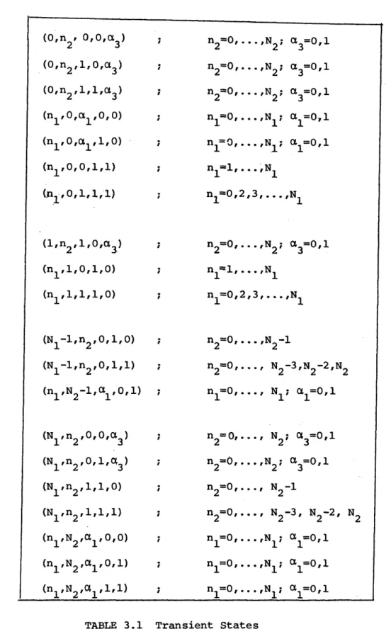
results are presented in Table 3.1.

There are two kinds of transient states.

The first cannot be

reached from any other state (i.e., the probability of transition

from any other state to that state is 0).

An example is a state in

which .i

= 0 and ni

-

₁

= 0. Table 2.2 indicates that if i.

(t+l) = 0

and ni l(t) > 0, then ni_ (t+l)

>

ni

_{l (}

t).

Thus, the only way for

ni l(t+l) to be 0 is for ni l(t)

=

0. Table 2.1, however, indicates

that if nil(t)=0, the only way for

i.

(t+l) to be 0 is for ai

(t)=0.

Therefore, a state in which ai=0 and nil

=0 may only be reached from

states in which a

=0 and n

i

1=0.

If, in addition, ai

1

=l and machine

1

(0,n2, 0,O,c3) n2=0,...,N2; a3=0,1 (O,n2,1,0,t) 3 ; n2=0,...,N2; a3=0,1 (O,n2,1,1,a3) ;n2=0, ,N2; 3=0,1

(nl,O,al,O,O)

n =,0..,N1 ;l=,

1 ,...,N

₁

z

₁

=0

1 (n1 10,ct1 11,O) nl=0,... ,N 1; a1=o, (nl',O,1,'.1) ; nl=0,2,3,..',N₁ (ni 1,,Ll,0) ; n1=0,2,3,...,N1 (nl, 1,0,1O) ; nl-l, ... ,N 1 (Nl-l,n2,0,1,0) ; n2=0,...,N2-1 (Nl-1,n2

0,1,1)

; n2=0,..., N2-3,N2-2,N 2 (nlN2-lalo,l) ; nl=0,..., N1; 1a=o0,1 (Nln2,0,0,o)3 ; n2=0,..., N2; C3=0,1 (N l,n2, ; a0,1 (Nln2,1,1,0) ; n2=0,..., N2-1 (Nln2,1,1,1) ; n2=0,..., N2-3, N2-2, N2

(nl,N2,al,0,0) ; nl=O,*.,N1;

al=o,1

(nlN2

l,

o,1)

;

nl=O, ,N1; ..

al=o,1

(nlN2,~l,1,1) ; nl=O,...,N1; al=0,1

i-1 is not starved, this state cannot be reached from another state,

since an operating upstream machine would raise the level in storage

i-i.

Similar results apply to the case in which ai=0 and n.=Ni.

The remaining transient states are reachable only from other transient

states. For example, consider states in which ni_

2

>0, ai =l,, ni.l=l,

ai=0. Table 2.2 implies that at the previous time step, storage i-2 had

one more piece and ni_

=

0. But this implies that at the previous time

step ai= 0 because machine i cannot fail when storage i-l is empty (see

Table 2.1).

Thus, at the previous step, ni

0 and .ai=

0, which has

been established as transient.

The full list of transient states, which appears in Table 3.1, can

be established by the following rules.

(i) States where n

i-l

₌

and

.= 0, or

a.=0

and n.

=N.

are

i-l

1 1 1 1

transient. This is because a starved or blocked machine cannot fail

(Section 2.3).

(ii) States where machine i-1 is operating (i.e., not idle) ni 1=

and ai.=; or ai= O, n.= N.-l and machine i+l is operating, are transient.

I 1 1 1

This is because machine i could not have failed if nl

=

0 or n.=N., and

1-1 1 1

an operating machine upstream or downstream would have incremented the

storage by plus or minus one, respectively, in the cycle during which machine

i failed.

(iii)

States where machine i-1 is operating and ni l=0; or ni l=Ni l

and machine i is operating are transient. This is because an operating

machine upstream or downstream would increment the storage by plus or minus

one, respectively, since by assumption (vi) of Section 2.3, machine

transi-tions precede and determine storage transitransi-tions.

It is important to note the following exceptions:

(i)

(1,0,1,1,1) can be reached from (0,0,0,1,1)

(ii)

(1,1,1,1,0) can be reached from (0,1,0,1,1).

(iii)

(N

₁

, N2-1,1,1,1) can be reached from (N

1

, N2,1,1,0).

(iv)

(N -1, N2-1,0,1,1) can be reached from (N -l,N2,1,1,0).

These states are thus not transient.

Finally, the fact that machine 1 is never staryed and-machine 3

(for k= 3) is never blocked (Section 2.3) must be considered in deriving

the transient states.

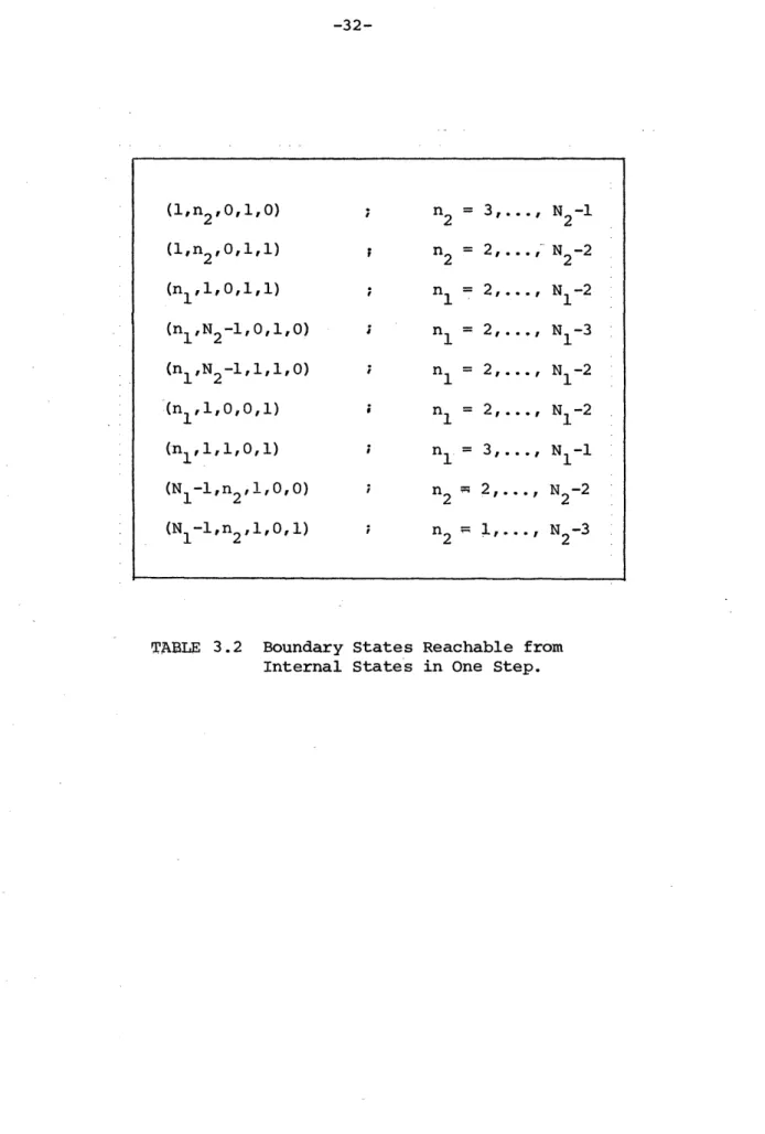
3.3.2 Boundary States Reachable from Internal States in One Step

It is easy to derive

E

expressions for certain states. For example,

the transition equation for p(1,2,0,1,1) is

p(1,2,0,1,1) = (1-ri)r

2

r

3

p(2,2,00,,0)

+ (1-rl)r2(1-p3)p(2,2,0,0,1) + (1-r1) (1-p2)r3p(2,2,0,1,0) +

(l-r

_{1 )}(1-p2 )(1-p3)p(2,2,0,1,1) + Plr2r3p(2,2,1,0,0)

+ plr2(1-p

3

)P(2,2,1,0,1)

+ p₁(l-p2)r3p(2,2, 1

,

1

O

0) +

pl

(l-p

2

)l-P

3

)p(2,2,l,l,l)

(3.30)

All the states on the right hand side of (3.30) are internal. The

co-efficients are the transition probabilities from states (n

1

, n

2

2

,

l', 2'

a3) to (nl-1, n

2

, 0,1,1), where nl and n

2

(i.e., the initial storage

levels) are internal.

If (3.21) is substituted into (3.30) and the

resulting expression is simplified using the -parametric equations, it is

seen that a natural choice for E(1,2,0,1,l,U) is the internal form

(1,2,0,1,1,U) = X

1

X

2

Y

2

Y

3

(3.31)

Similarly, it can be shown that

f(1, n2, 0,1,1,U) = X1X22Y2Y3

(3.32)

for all 2 < n2 < N2-2. The relation between (3.31) and (3.32) is generalized

in Section 4.2.

The same reasoning shows that the internal form is an appropriate

choice for the boundary states in Table 3.2.

(1,n2,0,1,0) n2 3,..., N2-1 (1,n2,0,1,1) n 2,..., N2-2= 2 (n1l,l,O,,1) nl = 2,..., N1 -2 (nl,N2-1,0,1,O) n1 = 2,..., N1-3 (nl,N2-1,1,1,O) n1 = 2,..., N1-2 1(nl,1,0,0,1) n1 = 2,..., N1-2 (nl 1, 1, 0,1) ;nl = 3,..., N-1 (N1-l,n2,1,0,0) n2= 2,..., N2-2 (Nl-l,n2,1,0,1) n₂ 1,..., N2-3

TABLE 3.2 Boundary States Reachable from Internal States in One Step.

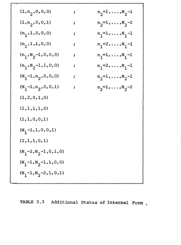
3.3.3 Other Expressions of Internal Form

The expressions derived in Sections 3.3.1 and 3.3.2 are the only ones

that are determined unambiguously, once the internal expressions are chosen.

The remaining expressions must be derived using guesswork and imagination.

In a sense, there are no correct expressions; the objective here is to

find expressions that satisfy as large a set of transition equations as

possible.

To guide guesses, numerical results were obtained for a case in

which N

₁

=N

2=10 (Gershwin and Schick [1977]) by iterative matrix

multi-plications (the power method; see Schick and Gershwin [1978]). It was

observed that several boundary state probabilities, in addition to those

described in Section 3.3.2, appeared to be comparable to adjacent internal

state probabilities. Generalizing from the case studied, the internal

form is assumed for the states listed in Table 3.3.

3.3.4 Other Expressions

To obtain 5(s,U) expressions for other states s, other approaches

must be used. One fruitful method has been to look for pairs of equations

that involve the same pair of unknown states, and in which all other states

have expressions already determined. For example, consider the transition

equations for (1,1,0,0,1) and (1,2,0,0,0). (See Appendix A.)

The initial

states are all of the form (1,2,al

₁

,ac2,a

₃

). Of these, S(1,2,1,0,0,U) = 0

and E(1,2,1,0,1,U) = 0 (from Table 3.1), E(1,2,0,1,1,U) has internal

form (from Table 3.2), and E(1,1,0,0,1,U), E(1,2,0,0,0,U), E(1,2,0,0,1,U),

and -(1,2,0,1,0,U) have internal form (from Table 3.3).

From these equations, and by performing considerable simplifications

using the parametric equations (3.17) and (3.19), the following are

obtained:

2

X X2Y

E(1,2,1,1,0,U)

1 2 1

(l-r

+ p Y)

(3.33)

P2

2

22

2

X X2Y (1,2, 1, 1, 1,U) = _{1 2 1} (1-r + p Y )Y (3.34) P2

(ln2

°)

;

2=1,.. .,N

2-1

(1,n2,0,0,1) n2=1,. .,N2-2 (n

,1,0,0,0)

; (nl1,1,O; nl=2, . . .,N1-1 (n1,N2

_(n

-1,0,0,0) nll.... ,Nl 1

,

N

2

-1,0,

O,

0

)

1

(nl,N2-1,1,0,0) ; nl=2, . . .,N1-1 (N

₁

-l,n2

₂

0,0,0) n

₂₂₌

2 1,. _l

_,N

,N2 2

-1

(N1_-l,n ₂ 0,0,1) n2=1, . . .,N ₂-2

(1,2,0,1,0)

(1,1,1,1,0)

(1,1,

0,

0,1)

(N -1,1,0,0,1)

(2,1,1,0,1)

(N_{1 - 2} ,N2-1,0,1,0) (N1 ,N2-1,1,0, 0) (N-1,N2-2,1,0,1)

Comparison of the transition equations for (1,1,0,0,1) and (1,2,0,0,0)

with similar equations involving higher storage levels suggests the

generalization of equations (3.33) and (3.34):

n2

XX

Y

(l,n2,1,1,0,U)

2

(1-r

2

+ P2Y2)

(3.35)

n

n

2

=2,...,N

2

-1

E(ln

₂

l'l'l'U)

=

P

2

(l-r

2

+

P

2

Y

2

)Y

3

(3.36)

It must be emphasized that this procedure is more nearly art than

science, and is a way of organizing guesswork which must be verified

later. According to the procedure and data described in section 3.3.3,

the expression for E(l,n2,1,1,0,U) in (3.35) might also apply for n

2

= N

2

.

However, there is no justification for this in the transition equations,

and to choose this expression for this state would create additional

non-zero errors g(s,U).

The objective is to maximize the number of

transition equations that are satisfied identically, i.e., to minimize

the number of states for which g(s,U) is not zero for all U satisfying

the parameteric equations (3.17) - (3.19). Consequently, E(1,N2,1,1,0,U)

is chosen differently.

Note that E(0,2,0,1,0,U) and ~(0,2,0,1,1,U) expressions were

found using the (1,2,1,1,1) equation, which actually involves the

(0,3,0,1,0) and (0,3,0,1,1) states.

It was assumed, as discussed in

Section 4.2, that

E(0,3,0,1,0,U) = X

2

E(0,2,0,l,0,U)

(3.37)

E(0,3,0,1,1,U) = X2E(0,2,0,1,1,U)

(3.38)

Other states whose expressions are found by solving two equations

in two unknowns are displayed in Table 3.4. The second column of this

TABLE 3.4 Expressions Obtained in Pairs

States Equations Generalizations

(1,2,1,1,0) (1,1,0,0,1) (1,n2,1,i,0), n2=2,...,N2-1 (1,2,1,1,1) (1,2,0,0,0) (1,n2,1,1,1), n2=2,...,N2-1 (1,1,0 (1,1,0,1,1,0,0,0) (1,1,1,1,1) (2,1,1,0,0) (2,1,0,1,1) (1,2,0,1,0) (n1 ,,0,1,1), nl=2, ..,N1-2 (2,1,1,1,1) (2,1,0,0,0) (n1,l,1,l,1), nl=2,...,N1-2 (2,0,0,0,1) (1,1,01,1) (nl ,0,0,0,1), nl=2, ... ,N-1 (2,0,1,0,1) (2,1,1,1,1) (n1,0,1,0,1), nl=2,...,N -1 (0,2,0,1,0) (1,2,1,1,0) (0,n ,0,1,0), n2 =2,...,N2 -i2 (0,2,0,1,1) (1,2,1,1) ( (0,n2 ,0,1,1), n2=2,...,N2-1 (0,1,0,1,0) (1,1,1,1,0) (0,1,0,1,1) (0,1,0,1,0) (N1-l,2,1,1,0) (N1-2,2,0,1,1) (N -l,n2 ,1,1,0), n2=2,...,N2-1 (N -1,2,1,1,1) (N -1,2,0,0,0) (N -l,n2,1,1,1), n2=2,...,N -1 (Ni,2,1,0,0) (N -1,2,1,1,1) (N

2

1,0,), n2-2 'N -2 (N1,2,1,0,1) (Nl,3,1,1,0) (Nl,n2,1,0,1), n=2,..,N2-2 (2,N2-1,0,1,1) (2,N2-1,0,0,0) (nl,N2-1,0,1,1), nl=2,...,Nl-1 (2,N2-1,1,1,1 (2,N2-2,0,0,1) (nl,N2-1,1,1,1), nl=2,...,Nl-1

TABLE 3.4 (Cont'd)

States Equations Generalizations

(1,N2,0,1,0) (1,N2-1,0,1,1) (nl,N2,0,1,0), nl ,...,N 1-2

(1,N2,1,1,0) (2,N2-1,1,1,1) (ni,N2,1,1,0), n =l,...,N -2

(N-1,N2' 0,1,0) (N -1,N2-1,0,1,1)

table lists the equations used, and the last column generalizes these expressions in the manner described above.

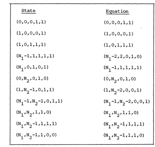
Table 3.5 lists states whose expression can be obtained singly after express-ions for certain other states are available. The complete

list of expressions appears in Appendix B.

3.4 Reduction of the System of Equations

A small number of boundary transition equations were used to generate each expression discussed in Section 3.3. It is possible to show, using the parametric equations, that these expressions satisfy many of the remaining transition equations identically.

A significant number of boundary equations, however, are not satisfied identically. The states that these transition equations lead to are

called "odd" states and are discussed in greater detail in Section 4.2. The set of odd states is called Q. The number of states 2 in Q is much smaller than M. In this section it is shown how the Markov chain may be solved by solving a set of Z linear equations, rather than M. These linear equations are constructed in finding a linear combination of (U.) which satisfies all the transition equations, including those

leading to states in Q.

For the Markov chain described in section 2.4,

p

= Tp (3.39)

or

(T-I)p (3.40)

where I denotes the identity matrix. For a general k- stage transfer line, the boundary state probabilities are expressed as a sum of terms, analogous to the sum of products for internal state probabilities in equation

(3.6):

p(s) = ECj i(s,Xlj... ,' Xk-l,j'Ylj Ykj (3.41)

TABLE 3.5 Expressions Obtained Singly State Equation (0,0,0,1,1) (0,0,0,1,1) (1,0,0,0,1) (1,0,1),0,0,1) (1,0,1,1,1) (1,0,1,1,1) (N₁-1,1,1,1,1) (N1-2,2,0,1,0) (Ni, 0,1,0,1) (N -1,1,1,1,1) (O,N2 0,11,0) (0,N2 01,0) (1,N₂-1,0,1,1) (1,N2-2,0,0,1) (N₁-1,N2-1,0,1,1) (N -1,N2-2,0,0,1) (N₁,N2 1,1, 0) ( 1,N2,1,1,0) (Nl,N 2 -1,1,0,0) (N1 ,N2-11,1,1) (Nl,N2-1,1,0,0) (Nl,N2-11,1,10)

The S(s,U) expressions are derived in Section 3.3. Note that (3.41) reduces to (3.6) when E(s,U) is given by (3.22). Following (3.41), the probability vector p may be rewritten as

Z'

p

=

E

Cj

_

(Uj) (3.42)

j=l

where i(U) is a vector whose components are E(s,U).

The number of states

M is given by equation (2.4), and Uj, j

=1,..., I' are V' distinct

solutions of the parametric equations. Substituting (3.42) into (3.40),

(T- I) E Cj(Uj) . (3.43)

j=l

Defining the vector C as

C₁

C C₂ (3.44)

and the matrix ~ as

= [(U 1) (U2) ,, g(U,)3 (3.45)

equation (3.43) is rewritten as

(T-I);C = 0 (3.46)

System (3.46) has a nonzero solution if the matrix (T-I)E has

rank less than or equal to V'-l. Equation (2.14) provides an additional condition on C through (3.41) which requires that C be nonzero. A

unique solution is determined if the rank of (T-I)E is exactly equal to

V-l.

Because the expressions r(s,U) satisfy most transition equations, most components of the vector (T-I)_(Uj) are identically equal to zero for any U. that satisfies the parametric equations. For example, in the three-stage line with storage capacities N1= N2 = 10, 898 components out

of the 968-vector are identically zero. Those that are nonzero correspond to odd state entries in i (U). If

2'

is taken to be the number of rows

not automatically satisifed, i.e., Z' =, then the system of equations (3.46) has a unique solution C, once a set of £ distinct U. is chosen. The

system in (3.46) can be reduced by computing only those Z rows of (T-I)E that are not satisfied identically. The new reduced-order system can be

written-BC = 0 (3.47)

where B consists of thenon-zero rows of (T-I)S and is .xR rather than MxM. This system is analyzed in Section 4.2.