PSINES: Activity and Availability Prediction for Adaptive Ambient Intelligence

HAL Id: hal-02943970

https://hal.archives-ouvertes.fr/hal-02943970

Submitted on 21 Sep 2020

HAL is a multi-disciplinary open access

archive for the deposit and dissemination of

sci-entific research documents, whether they are

pub-lished or not. The documents may come from

teaching and research institutions in France or

abroad, or from public or private research centers.

L’archive ouverte pluridisciplinaire HAL, est

destinée au dépôt et à la diffusion de documents

scientifiques de niveau recherche, publiés ou non,

émanant des établissements d’enseignement et de

recherche français ou étrangers, des laboratoires

publics ou privés.

Adaptive Ambient Intelligence

Julien Cumin, Grégoire Lefebvre, Fano Ramparany, James Crowley

To cite this version:

Julien Cumin, Grégoire Lefebvre, Fano Ramparany, James Crowley. PSINES: Activity and

Availabil-ity Prediction for Adaptive Ambient Intelligence. ACM Transactions on Autonomous and Adaptive

Systems, Association for Computing Machinery (ACM), 2020, 15 (1), pp.1-12. �10.1145/3424344�.

�hal-02943970�

PSINES: Activity and Availability Prediction for Adaptive

Ambient Intelligence

JULIEN CUMIN, GRÉGOIRE LEFEBVRE, and FANO RAMPARANY,

JAMES L. CROWLEY,

Autonomy and adaptability are essential components of ambient intelligence. For example, in smart homes, proactive acting and occupants advising, adapted to current and future contexts of living, are essential to go beyond limitations of previous domotic services. In order to reach such autonomy and adaptability, ambient systems need to automatically grasp their users’ ambient context. In particular, users’ activities and availabilities for communication are valuable pieces of contextual information that can help such systems to adapt to user needs and behaviours. While significant research work exists on activity recognition in homes, less attention has been given to prediction of future activities, as well as to availability recognition and prediction in general. In this paper, we investigate several Dynamic Bayesian Network (DBN) architectures for activity and availability prediction of occupants in homes, including our novel model, called PSINES (Past SItuations to predict the NExt Situation). This predictive architecture utilizes context information, sensor event aggregations, and latent user cognitive states to accurately predict future home situations based on previous situations. We experimentally evaluate PSINES, as well as intermediate DBN architectures, on multiple state-of-the-art datasets, with prediction accuracies of up to 89.52% for activity and 82.08% for availability on the Orange4Home dataset.

CCS Concepts: • Mathematics of computing → Bayesian networks; • Human-centered computing → Ambient intelligence.

Additional Key Words and Phrases: Activity Prediction, Dynamic Bayesian Networks, Ambient Intelligence, Context-aware Services, Smart Homes

ACM Reference Format:

Julien Cumin, Grégoire Lefebvre, Fano Ramparany, and James L. Crowley. 2019. PSINES: Activity and Availabil-ity Prediction for Adaptive Ambient Intelligence. ACM Trans. Autonom. Adapt. Syst. 1, 1, Article 1 (January 2019), 19 pages. https://doi.org/10.1145/nnnnnnn.nnnnnnn

1 INTRODUCTION

Autonomous and adaptive systems have been an important vector of progress in work efficiency, scientific research, and quality of life. Clocks or mechanical calculators, which are some of the first examples of automated systems, allowed people to measure quantities or to perform calculations much more efficiently and accurately. Advances in information technologies and computer science have allowed the development of automation strategies for more complex tasks. In particular, the increasing sensing and computing capabilities of everyday objects has enabled new perspectives for automation.

One such perspective is that of home automation, where we aim to automate daily tasks, chores, or energy management in the home. Automatic regulation of heating and air conditioning, lighting control, or energy consumption management are examples of use cases first considered and de-veloped when home automation arose. However, these services often did not react properly with

Authors’ addresses: Julien Cumin, [email protected]; Grégoire Lefebvre, [email protected]; Fano Ramparany, [email protected], Orange Labs, 28 chemin du Vieux Chêne, Meylan, France, 38240; James L. Crowley, [email protected], Université Grenoble Alpes, Inria, CNRS, Grenoble INP, LIG, Grenoble, France. © 2019 Association for Computing Machinery.

This is the author’s version of the work. It is posted here for your personal use. Not for redistribution. The definitive Version of Record was published in ACM Transactions on Autonomous and Adaptive Systems, https://doi.org/10.1145/nnnnnnn.nnnnnnn.

respect to users’ expectations, and thus became more of a nuisance than a convenience [1]. Such inappropriate automation is a great barrier to adoption for home automation technologies.

One of the commonly given reasons for these inappropriate results is the difficulty of implement-ing autonomous adaptation strategies to the specificities and preferences of a particular household. In particular, it is often difficult to infer the needs of occupants of a home based directly on low-level sensor data. Moreover, automation for the sake of time saving is actually not often the main reason for the adoption of similar technologies in homes: users are commonly more interested in services that improve their quality of life instead. However, automation services are not the only kinds of services that can be provided in a home. Following Crowley and Coutaz’s definitions of home ser-vices in [1], classical home automation would often fall into tool service and housekeeping service categories, but not in advisor and media services, which provide information and suggestions to occupants, or extend their perceptual capabilities.

In this article, we focus on one other major aspect of the daily life of people, which is communi-cation. With recent technological advances, the number of communication modalities (through the internet, smartphones, etc.) and thus potential contacts has significantly increased, to the point where incoming communication attempts can become a nuisance. A home that manages incoming communications for its occupants can thus be a valuable service that improves quality of life. Such a service would fall into an advising category of service.

A communication assistance service could for example suggest appropriate moments for an outsider to call an occupant, based on that occupant’s availability to communicate. It could suggest appropriate modalities of communication or devices to reach an occupant: for example, if an occupant and their landline phone are on different floors, the assistant can suggest to call on their mobile phone rather than the landline phone. It could automatically delay the delivery of messages such as e-mails until the occupant is available, in order to reduce their mental load.

Such an autonomous communication assistant cannot provide a valuable service unless it has access to personal preferences and situations of its occupants. Indeed, it needs to automatically adapt to the availability of occupants for communication, which can greatly vary depending on the occupants’ identity, their daily routine, the current time, the place they are in, their mood, or even outside events. If this assistant did not offer such contextual adaptability, it would probably exhibit inappropriate behaviors and suggestions to outsiders in a manner similar to past home automation systems. Moreover, such a system needs to anticipate future activities of occupants, in order to give suggestions for future availabilities of occupants. Such autonomous context recognition and prediction capabilities allow not only the implementation of communication assistance, but also a multitude of other possible autonomous and adaptive services such as multimedia content suggestions, context-aware occupant agenda management, etc.

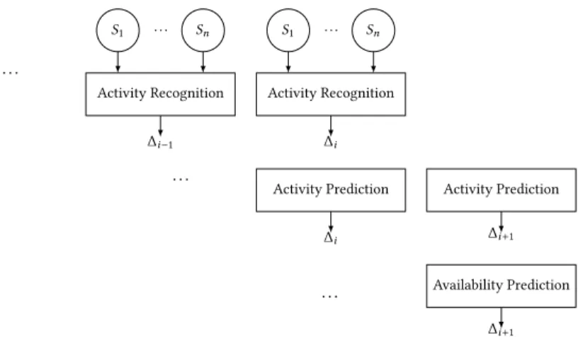
This communication assistant is thus a complex example of an autonomous adaptive smart home service that raises a number of algorithmic problems on activity recognition and prediction. We will thus use this example of communication assistance as the motivating service for all our contributions in this article. In particular, this service requires activity prediction as well as availability prediction capabilities (see Fig. 1).

Activity recognition.The problem of activity recognition in smart homes consists in automatically identifying the current activity of an occupant using only data collected by sensors installed in the home. Smart home sensors typically record low-level data such as temperatures, electrical consumptions, motion detections, door opening events, etc. Activities are complex sets of tasks performed by an occupant with a set goal, such as cooking, showering, sleeping, etc. Activity recognition must be as accurate as possible, so as to limit the possibility of providing inappropriate services that rely on activity information. However, recognizing such complex activities from

heterogeneous and individually poorly informative sensors is difficult. In particular, the relationship between activities and sensor data is highly dependent on occupants’ preferences, routines, and moods, as well as the topology of the home and the existing sensor installation.

Activity prediction.The problem of activity prediction (or forecasting) in smart homes, in our study, consists in automatically predicting, at the next situation timestep, the most likely occupant activity based on their past situations and their current situation. Routines of occupants are challenging to predict because they can highly vary from one person to the next, from one day to another, and unexpected changes can occur depending on the mood of occupants, which is generally unobservable. Activity prediction, in our case, is thus expected to only be able to correctly predict activities that fall under the different routines of occupants. In cases where occupants perform a sequence of activities completely outside of the ordinary (based on their personal ordinary routines), it is not expected that we will be able to predict, before any observation, such activities. They are by definition unpredictable, both in the common and technical sense. Nevertheless, routines of an occupant can still present high variability, both in terms of activity sequences and times of occurrence. It is the task of the predictor to take such variability into account.

Availability prediction.The problem of availability prediction (or forecasting) in smart homes, in our study, consists in automatically predicting, at the next situation timestep, an inhabitant availability value between a scale from not available for anyone to definitely available for anyone. The aim is thus to predict at the next timestep if an outside communication would inappropriately interrupt an occupant or not, based on their previous situations and current situation.

In this work, we propose an availability prediction system that employs a more general situation prediction system, called PSINES, which predicts the activity and availability of an occupant for the next timestep, using previous situations. Past activities at each timestep are derived from an activity recognition step. PSINES is a Dynamic Bayesian Network (DBN) architecture that extends a state-of-the-art prediction model with 4 contributions:

(1) we include sensor data through aggregate nodes, instead of limiting ourselves only to higher level context data.

Activity Recognition ∆i S1 ... Sn ... Activity Recognition ∆i −1 S1 ... Sn ... Activity Prediction ∆i+1 Activity Prediction ∆i ... Availability Prediction ∆i+1

Fig. 1. Availability prediction at timestep i+ 1 from previous sensor value sequences, previous activity

sequences and previous availability sequences. Activity Recognition is based on a set of home sensors S_kat

(2) our method goes beyond modelling activity as a first-order Markov process, to use higher order relations between activities, so that past activities can have a more meaningful impact on prediction of future activities.

(3) we explore the use of a latent node that models the cognitive state of the occupant, which in theory should be the main influence on future activities but which is unobservable in practice.

(4) we include availability prediction in our PSINES activity predictor model.

This paper is organized as follows: Section 2 presents a survey of activity prediction strategies in homes. Our PSINES (Past SItuations to predict the NExt Situation) method is then described in Section 3. This method integrates four approaches that improve the prediction accuracy of a state-of-the-art algorithm using context information and specificities of the home. Section 4 presents the results of experimental evaluations using several state-of-the-art datasets of home activities. Conclusions and perspectives are drawn in Section 5.

2 APPROACHES TO ACTIVITY AND AVAILABILITY PREDICTION

Two main approaches to activity prediction in the home can be found in the literature: sequence mining and machine learning. In opposition, availability prediction is classically performed by inference strategies. In this section, we review some works on each of these approaches.

2.1 Sequence Mining for Activity Prediction

Sequence mining refers to the prediction of activity by manipulation of sequences of symbols. This can include sequence matching, compression, item-sets mining, pattern mining, and association rule mining. For example, in a survey of activity prediction in homes by Wu et al. in 2017 [2], we exclusively find algorithms from these categories. This predominance is the result of a long history of research on the extraction of patterns in sequences of symbols, dating back to Shannon’s work on the entropy of information [3]. Several well-established algorithms for compression, itemsets mining, pattern mining that were designed for other applications can also be applied to the problem of activity recognition in homes. Classical examples of such algorithms include Apriori [4], Minepi and Winepi [5], FP-Growth [6], and Eclat [7].

2.1.1 Active LeZi.Gopalratnam and Cook propose in [8] a sequence prediction algorithm that relies on data compression techniques, called Active LeZi. This predictor is based on the LZ78 text compression algorithm, which incrementally parses sequences of symbols to construct a dictionary of symbol phrases. Drawbacks of LZ78 include slow convergence, which was already tackled by Bhattacharya and Das in [9] with the LeZi update technique. Active LeZi is an improvement on both LZ78 and LeZi update to address convergence slowness, by using sliding windows. The authors prove a number of theoretical results on the convergence rate and complexity of Active LeZi, compared to previous solutions.

The main application domain Gopalratnam and Cook apply Active LeZi to is smart home systems. In particular, they consider their approach suitable for predicting activities of occupants, which is useful for services such as home automation. In their experiments, they study the behaviour of Active LeZi, not directly on human activity prediction, but rather on interaction prediction. The goal is to predict, from a sequence of previous events, the next change observed by a device (e.g. a door sensor detects that its door is now opened). They show that Active LeZi can obtain reasonable prediction performance, especially when the top five predictions made by the algorithm are considered.

2.1.2 SPEED.In [10], Alam et al. present a sequence prediction algorithm called SPEED. Previous compression techniques such as Active LeZi, are based on general sequences of data and do not take into accounts the properties of home data sources and specificities in human behaviour. SPEED, on the other hand, is designed specifically for the problem of activity prediction in homes, and thus takes into consideration certain properties. For example, as this work limits itself to “On/Off” sensors, we can identify episodes of data collected between an “On” event and a “Off” event of one sensor, that correspond to home interactions. SPEED constructs a Decision Tree (DT) which contains the identified episodes in a sliding window over the data sequence. This DT corresponds to a finite-order Markov model and is used to infer the probability of occurrence of a specific symbol after having observed a specific window of data. Alam et al. present a number of theoretical results on the time and space complexities of SPEED. They show that it converges faster than Active LeZi and leads to more accurate prediction, while requiring more data storage for the DT.

2.2 Machine Learning Prediction for Activity Prediction

Some authors have proposed to use a combination of sequence matching techniques in conjunction with machine learning algorithms, which can adapt to data source specificity. In this case, sequence matching is used to extract well-supported patterns in the data to construct features, which are then used to train an algorithm in order to predict activities. The variety of home environments and user routines makes it unlikely that hand-crafted features, extracted using sequence mining, will actually be valuable to model activity prediction for all homes, let alone be optimal. Therefore, we find in the literature some works that directly use machine learning techniques, without any preliminary sequence matching. Most works are based on graphical models (e.g. HMM) as in [11, 12, 13, 14, 15, 16]. We also find some examples of deep learning approaches (e.g. LSTM (Long Short Term Memory neural networks)) applied to activity prediction, as in [17, 18, 19].

2.2.1 Discovering Behaviour Patterns.Fatima et al. propose in [20] a two-step module for activity prediction in homes. In the first step, sequence pattern mining is applied in order to discover temporal patterns of activity sequences. A support threshold allows to prune sequences of activities that are too infrequent in the dataset. According to the authors, this step allows to find significant behaviour patterns that occur frequently on different days, and that thus may be used to model the routine of occupants. In the second step, a Conditional Random Field (CRF) is employed to model activity sequences for activity prediction. CRF are generative probabilistic graphical models that allow to capture directed dependencies between variables, such as activities. Sufficiently supported sequences of activities found in the first step are used to train the CRF. In particular, Fatima et al. propose to only use supported sequences of 8 to 10 consecutive activities to predict future activities, and discard shorter supported sequences. They show that their two-step method leads to better prediction accuracy compared to a classical Hidden Markov Model (HMM).

2.2.2 Itemset Mining and Temporal Clustering.In [21], Yassine et al. propose a three-step process for activity prediction in homes. First, an itemset mining strategy is used to identify frequently supported patterns that relate activities to appliance usage in collected data. The extraction algo-rithm they use is based on Frequent Pattern Growth (FP-Growth) and is presented in more details in [22]. While the first step focuses on finding appliance-to-appliance and appliance-to-activity relationships, the second step is used instead to find appliance-to-time relationships. In particular, the goal is to discover, in recorded data, the usage time of appliances with respect to various temporal elements: hour of day, time of day, weekday, week of the year, month of the year. An incremental k-means strategy is used to cluster appliances with similar temporal usages together. Finally, the third step aims at predicting activities from these appliance-to-appliance frequent patterns and appliance-to-time relationships. Finally, they propose to use a Bayesian Network (BN)

in which these appliance and temporal associations are modelled in the BN structure. The BN can then predict the most probable future appliance usages.

2.2.3 CRAFFT DBN.Nazerfard and Cook present in [23] an activity prediction approach based on DBN (Dynamic Bayesian Network), called CRAFFT (CuRrent Activity and Features to predict next FeaTures). In this model, 4 input variables are used to predict the future activity: the current activity, the current place where the occupant is situated, the current time of day, and the current day of week. These variables are direct representations of 3 of the primary context dimensions in the home: activity, place, and time. The particularity of the CRAFFT DBN structure is that the future activity is not directly predicted from these 4 contextual variables. In fact, the future place, the future time of day, and the future day of week of the next activity are predicted from these 4 variables. Then, the future activity is predicted using these 3 new inputs in addition to the initial 4 observations. Nazerfard and Cook, through an experimental study, argue that this particular 2-step DBN architecture leads to better activity prediction performance than a more naïve direct prediction from the 4 current context variables.

2.3 Availability inference

Few works tackle the problem of inferring the current availability of occupants at home, let alone predict their future availability. In the literature, we find that most works related to availability estimation are focused on professional environments or smartphone usage. These applicative environments are indeed more constrained and controlled than homes in which occupants have complete freedom over their activity and thus availability. Nevertheless, we do find some works that discuss availability inference, with two different major approaches: availability inference from sensor data, and availability inference from higher level context information such as activity. We review in this section two such papers that illustrate those categories.

2.3.1 Estimating Availability Through Audio-Visual Features.Takemae et al. propose in [24] an availability inference approach to help manage remote communication attempts in the smart home, much like our communication assistance service example. This approach relies on audio and visual data, on which they propose to extract a number of audio-visual features: voice power, frequency of changes in voice power, motion near a table area, changes in the location of occupants, etc.

Availability is then estimated using a support vector regression algorithm. Their experiments highlight some correlations between truth values of availability and availability computed by their approach. These results suggest that audio and visual data provide some insight on the availability of occupants in homes.

2.3.2 Correlations between Context Dimensions and Availability.Nagel et al. report in [25] a set of statistical studies on the link between availability for communication at home and other context dimensions. In particular, they study the influence of identity, place, activity, and companionship (e.g. the number of people with the target occupant) on availability for communication. Experimental results show that some occupants are more often available than others, that some places are highly correlated to availability while other places are not, and that some activities are useful to infer availability.

2.4 Discussion

The large corpus of work on sequence matching techniques, compression algorithms, itemsets mining, etc., can be transferred on the issue of activity and availability prediction. We generally have a good understanding of the behaviour and complexities of such techniques, which can offer some guarantees on a prediction system based on such algorithms. On the other hand, these

approaches are generally fairly rigid, in that they aim at finding temporal relationships in data regardless of the actual environment in which these data were recorded. Therefore, some works use sequence matching in order to construct some features from data, which is then used to train a machine learning algorithm that performs the actual activity prediction step. In approaches based on machine learning, it seems that most techniques used rely on graphical models such as CRF or DBN. These algorithms typically include explicit temporal relationships between elements of the model, which makes them well-suited for prediction problems, compared to other approaches such as MLP (Multi-Layer Perceptron) or SVM (Support Vector Machine), where temporality is not modelled.

The CRAFFT predictor [23] presents a particularly interesting approach. This predictive ar-chitecture uses context information in the form of activity, place, time of day, and day of week variable nodes in a DBN. Based on Nagel et al. [25] results on availability inference using context information, it seems promising to include availability information in such a predictive model. In this work, we thus choose to extend CRAFFT, based on home heuristics, in order to improve activity prediction accuracy while also including availability prediction capabilities. We present these extensions in the next section.

3 CONTEXT-BASED ACTIVITY AND AVAILABILITY PREDICTION 3.1 DBN for Activity and Availability Prediction

In this section, we introduce the basis for our contributions to the problems of activity and avail-ability prediction. We then present our intermediate contributions: SCRAFFT, NMCRAFFT, and CSCRAFFT models. We finally present our final model: PSINES.

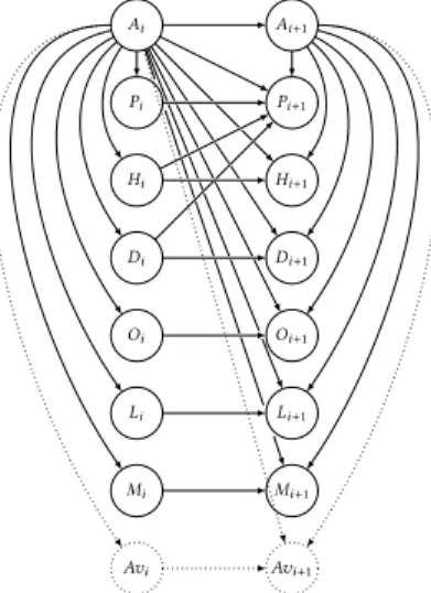
3.1.1 CEFA and CRAFFT DBN.Nazerfard and Cook introduce in [23] the CEFA (CurrEnt Features and activity to predict the next Activity) and CRAFFT (CuRrent Activity and Features to predict next FeaTures) DBN topologies, which we illustrate on Fig. 2 and 3, aimed only at the problem of activity prediction. Four variable nodes are introduced in this DBN architecture, ∀i ∈ {1, ...,T }:

• Ai, the Activity class performed at timestep i;

• Pi, the Place (in our case, the room) where the activity occurs at timestep i;

• Hi, the Hour of the day when the activity occurs. These values are discretized into 6 ranges

of hours: [0, 3], [4, 7], [8, 11], [12, 15], [16, 19], and [20, 23];

• Di, the Day of the week when the activity occurs, from 1 (Monday) to 7 (Sunday).

Here, Nazerfard and Cook define a timestep i as the window of time that begins with the start of activity Ai and ends when this activity stops. In our contributions to extend this model, we will

use the same definition of a timestep. Predicting future activities based on windows of time with fixed durations is a related but different problem, which is more akin to activity segmentation and activity recognition. In our work, we aim to predict the sequence of activity instances, segmented from one another, based on an underlying daily routine which we hope to model using a DBN.

The choice of edges in CRAFFT between nodes in the same timestep and edges between two consecutive timesteps relies on empirical observations by Nazerfard and Cook on home datasets. Examples of situations are given to justify, for example, the introduction of edges between Hi and

Pi+1or Di and Pi+1. In the CEFA architecture, the future activity Ai+1is directly predicted from

the currently observed features Ai, Pi, Hi, and Di. On the other hand, in the CRAFFT architecture,

the future activity Ai+1is not directly predicted from the observed variables (Ai, Pi, Hi, and Di).

Instead, a first step consists in predicting the contextual features of the next activity Pi+1, Hi+1, and

Ai Ai+1

Pi

Hi

Di

Fig. 2. Activity Prediction: Topology of the CEFA DBN as reported in [23]. Ai Pi Hi Di A_i+1 P_i+1 H_i+1 Di+1 Avi Avi+1

Fig. 3. Activity and Availability Prediction: Topology of the

CRAFFT DBN between timesteps i and i+ 1. Dotted nodes

and arrows are optional if only activity prediction is performed.

In their experiments, the authors show that CRAFFT is significantly more accurate for activity prediction than CEFA, on 3 datasets of activities in homes. They also show that CRAFFT is more accurate than standard classifiers such as SVMs and MLPs used as predictors. In Section 4.1, we reproduce these experiments on 5 new datasets of activities in homes to see if the same observations can be made.

We propose to add a new 5th_{variable Av}

i modelling occupant availability. As mentioned in our

motivations, in Section 1, our final goal is also to predict inhabitant availability status based on activity prediction in order to adapt communication services. Predicting inhabitant availability implies adding availability nodes, denoted by Avi and Avi+1, in our DBN architectures. Following

preliminary experiments, we design the prediction of inhabitant availability at timestep i + 1 as being dependent of 3 main nodes: availability at timestep i, activity at timestep i, and activity at timestep i + 1. These dependencies model our intuitive idea that availability is greatly influenced by activity and by previous availability.

3.2 Beyond CRAFFT: PSINES and Intermediate Models In the following section, we present our 4 contributions.

3.2.1 SCRAFFT: Sensor-Enhanced Prediction.In activity recognition, much of our input data comes from sensors installed throughout the home. In CRAFFT, such sensor data are not part of the DBN topology. Yet, the information of current activity (and possibly current place, at least in our place-based activity recognition approach), which are main variables of the CRAFFT model, are typically inferred from these sensor data. As such, additional information about sensors can be introduced in the CRAFFT topology at no cost, since these sensors are already necessary for the activity recognition step.

Therefore, we propose the SCRAFFT (Sensors CRAFFT) DBN, where new nodes are introduced to represent sensor aggregates. We illustrate a certain version of SCRAFFT on Fig. 4. In this version of SCRAFFT, we use 3 new variables:

• O_i, the number of Openings of doors, cupboards, etc., during the activity at timestep i; • L_i, the number of Light events recorded during the activity at timestep i;

Ai Hi Di Oi Li Mi Ai+1 Pi+1 Hi+1 Di+1 Oi+1 Mi+1 Pi Li+1 Avi Avi+1

Fig. 4. Activity and Availability Predic-tion: Topology of SCRAFFT DBN between

timesteps i and i+ 1. Dotted nodes and

ar-rows are optional if only activity prediction is performed. Ai −1 Ai −2 .. . ... Ai Pi Hi Di Ai+1 Pi+1 Hi+1 Di+1 Avi Avi+1

Fig. 5. Activity and Availability Prediction: Topology of

3-NMCRAFFT DBN between timesteps i −2 and i + 1. Dotted

nodes and arrows are optional if only activity prediction is performed.

We propose to quantize each sensor variable into 3 categories, based on the number of activa-tions of the sensor during the whole activity: “low” activation, “medium” activation, and “high” activation. Following statistical analysis, quantization thresholds were set such that for each sensor, all categories of activation roughly have the same number of instances. We chose 3 categories after experiment different numbers of categories on validation data. These 3 sensor aggregate nodes influence their own future value at the next timestep, and are conditionally dependent on the activity node. A 2-step prediction scheme is used with Oi+1, Li+1, and Mi+1being predicted along

with Pi+1, Hi+1, and Di+1before predicting Ai+1.

3.2.2 NMCRAFFT: non-Markovian Prediction.Standard DBN respect the first-order Markov prop-erty. As such, the CRAFFT model, which is a DBN, respects the same propprop-erty. Therefore, in that predictive model, the future activity to predict is only influenced by the immediately preceding timestep. In particular, it is only influenced by the immediately preceding activity performed, and not by any other previous activities.

We thus introduce the NMCRAFFT (Non-Markovian CRAFFT) topology for activity prediction, in which the future activity depends not only on the immediately preceding activity, but on the last d activities that occurred. We call d the non-Markovian depth of the d-NMCRAFFT model. We expect that, while increasing the non-Markovian depth slightly will improve prediction accuracy, overfeeding the predictor with past information (i.e. using large values of d) may decrease its performance.

We illustrate the 3-NMCRAFFT structure on Fig. 5. We see that Ai+1is conditionally dependent

not only on Ai, but also on Ai −1and Ai −2, since the non-Markovian depth used here is 3. In addition,

Ai is also dependent on Ai −2, for symmetry reasons.

3.2.3 CSCRAFFT: Modelling Occupant Cognitive States.We assume that the main influence on transitions from one activity to another is occupants themselves: their will, their mood, their behaviour, etc., will ultimately drive them to perform an activity. In many cases, they will perform

Ci Ci+1 Ai Pi Hi Di Ai+1 Pi+1 Hi+1 Di+1 Avi Avi+1

Fig. 6. Activity and Availability Predic-tion: Topology of CSCRAFFT DBN between

timesteps i and i+ 1. Dotted nodes and

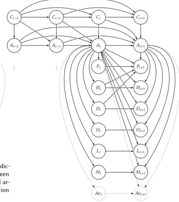
ar-rows are optional if only activity prediction is performed. Ci −2 Ci −1 Ci Ci+1 Ai −1 Ai −2 .. . ... Ai Hi Di Oi Li Mi Ai+1 Pi+1 Hi+1 Di+1 Oi+1 M_i+1 Pi Li+1 Avi Avi+1

Fig. 7. Activity and Availability Prediction: Topology of PSINES DBN between timesteps i −2 and i +1. Dotted nodes and arrows are optional if only activity prediction is performed.

activities in a logical sequence. However, when the occupant’s mood or will has a noticeable effect on the activity they choose to perform (e.g. “Telephoning” after “Cooking”), such sensor and context-based prediction strategies might not be as accurate.

The literature proposes some works that include the mental state of a user [26, 27]. Other studies of Mihoub and Lefebvre in [28], tackle the problem of feedback prediction for public presentations through the use of a DBN architecture that includes the cognitive state of the orator. They show that the inclusion does increase the feedback prediction accuracy of the model. This node can be latent, that is, unobserved and thus predicted. They also propose to discover a priori the observations for this cognitive state node, by applying different clustering algorithms on the rest of the data sources, with varying number of clusters (and thus cognitive state classes).

We propose the CSCRAFFT (Cognitive State CRAFFT) DBN, in which a node representing the cognitive state of the occupant is introduced in the standard CRAFFT structure. We illustrate CSCRAFFT on Fig. 6. The cognitive state of the occupant Ci at timestep i influences the current

and future activity Ai and Ai+1, as well as their future cognitive state Ci+1. This node can either be

latent or observed following a clustering step, as in [28].

3.2.4 PSINES: Past SItuations to predict the NExt Situation.Our final contribution to the problem of activity prediction consists in a model which combines the contributions of the previous 3 proposed models: SCRAFFT, NMCRAFFT, and CSCRAFFT. This new model, which we call PSINES, is thus a DBN whose topology is initially based on CRAFFT and that includes sensor aggregate nodes,

non-Markovian edges between activities, as well as cognitive state nodes. We illustrate PSINES on Fig. 7. In this combined model, we extend the non-Markovian structure of edges between activity classes to the cognitive state nodes. Indeed, since these nodes directly influence activities, it seems natural that they follow the same non-Markovian pattern.

Partial combinations of models are also possible. For example, one can combine NMCRAFFT and CSCRAFFT, and not include sensor aggregate nodes from SCRAFFT. We will still refer to such partial combinations as PSINES. In experiments, different combinations of models can thus be used for different homes, depending on the improvements observed on each model separately from the others. For example, if the occupant of a particular home holds very erratic and changing routines, the inclusion of NMCRAFFT might be detrimental to prediction performance; we would thus not include it in PSINES for that particular home. For another home where the occupant follows very structured routines, NMCRAFFT should lead to better prediction accuracy; in that case, we would thus include it in PSINES.

4 EXPERIMENTS

For these experiments, we used 5 of the CASAS datasets1_{[29]: HH102, HH103, HH104, HH105,}

and HH106. Each of these 5 datasets contains the labelled activities of a single occupant, along with collected sensor data. These 5 datasets were all collected during the same time period (June to August 2011): as such, we can use the same training protocol for all datasets, and more meaningful comparisons from one dataset to the other can be made. The datasets respectively contain 30, 28, 32, 30, and 33 different activity classes (the vast majority of which are shared between datasets), such as “Sleep”, “Bathe”, or “Watch TV”. In these datasets, we generally do not have information on the location of the occupant. As such, the place node in the tested models will always have a constant value of 1. We use a realistic temporal training protocol, where the first weeks of data are used as a training set and a validation set, and where the last weeks are used as the test set. On the CASAS datasets here, which all span the same time period, the training set spans from June 20, 2011 to July 10, 2011; the validation set spans from July 11, 2011 to July 17, 2011; the test set spans from July 18, 2011 to August 7, 2011.

For the last experiments in Section 4.5 on PSINES, we also used the Orange4Home2_{dataset [30],}

using respectively the first two weeks, the third and the last week as training, validation and test datasets.

In the following sections, a result in bold in a table indicates that this is the best result on a certain dataset for the particular experiment reported in the table.

4.1 Activity Predictions with Classifiers, CEFA, and CRAFFT

We report in Table 1 the prediction accuracy of the CRAFFT and CEFA models introduced in [23]. We also report in this table the prediction accuracy of a MLP, a SVM, and a BN, whose input vector contain the same features as the CRAFFT and CEFA models (previous activity, place, hour of the day, day of the week). Prediction performance seems to highly vary from one CASAS dataset to another: for example, future activity is accurately labelled on average 47.69% of the time on the HH103dataset, while we only reach an average accuracy of 17.10% on the HH102 dataset. This suggests that the inherent difficulty of each dataset is quite different among the 5 CASAS datasets we chose. This difficulty probably stems from occupants themselves: it will be easier to predict future activities for occupants with highly regular routines compared to occupants with more erratic routines. Nevertheless, this first set of experiments allows us to empirically verify the claims 1_{http://casas.wsu.edu/datasets}

Table 1. Activity prediction accuracy of the CRAFFT and CEFA DBN described in [23], as well as MLP, SVM, and BN using the same input data.

Predictor HH102 HH103 HH104 HH105 HH106 Mean SD MLP 17.74% 49.24% 31.91% 18.29% 25.36% 28.51% 11.59% SVM 20.44% 49.66% 33.21% 27.24% 26.38% 31.39% 9.99% BN 10.03% 45.25% 28.56% 11.75% 23.11% 23.74% 12.79% CEFA 16.20% 48.16% 28.67% 18.28% 20.47% 26.36% 11.69% CRAFFT 21.11% 46.13% 30.96% 25.22% 24.54% 29.59% 8.85% Mean 17.10% 47.69% 30.66% 20.16% 23.97% 27.91% 10.87% SD 3.96% 1.73% 1.82% 5.54% 2.05% 2.65% 1.39%

made by Nazerfard and Cook in [23]: we observe that, for all but the HH103 dataset, the CRAFFT DBN model is significantly more accurate than the CEFA DBN model (29.59% prediction accuracy on average compared to 26.36%). These results corroborate the findings of Nazerfard and Cook made on other datasets, that predicting future features before predicting the future activity is more accurate than directly predicting the future activity with DBN.

However, contrary to the results in [23], the CRAFFT DBN is not always more accurate than other classical classifiers here. On average, the accuracy of CRAFFT (29.59%) lies, in our experiments on the CASAS datasets, between the accuracy of a MLP (28.51%) and the accuracy of a SVM (31.39%). Therefore, we cannot confirm using our experiments that the CRAFFT DBN is significantly more accurate for activity prediction in homes compared to other prediction techniques that rely on classical classifiers.

All in all, we see that the prediction accuracy on any of the 5 tested datasets is quite low. The best predictor on the easiest dataset (the SVM on HH103) only reaches a prediction accuracy of 49.66%, which is an obviously unacceptable accuracy if we were to use such a system to provide context-aware services. Still, accuracies obtained here are significantly better than predicting uniformly at random the next activity: for a dataset of 30 classes (such as HH102 and HH105), such a random predictor would achieve an accuracy of 3.33%, which is significantly worse than all other predictors we tested.

Therefore, further work is required to greatly improve the prediction performance of such approaches. In the next experiments, we study the effect of some changes we can apply to the CRAFFT DBN architecture so as to improve its accuracy.

4.2 Sensor-Enhanced Activity Prediction

We report in Table 2 the prediction accuracy of the SCRAFFT model (presented in Section 3.2.1) on the CASAS datasets. Quantization bounds for the 3 sensor aggregates (Openings, Lights, and Motion) for each datasets were obtained by applying the k-means algorithm to obtain 3 clusters (corresponding to the 3 quantized values “low”, “medium”, and “high”) on the training part of the dataset. We can see that the SCRAFFT DBN is significantly more accurate than the CRAFFT DBN on all but the HH102 dataset. For example, on the HH103 dataset, the accuracy gap is greater than 4% (50.25% compared to 46.13%). This suggests that, in the majority of cases, sensor data, even when aggregated, brings valuable information to predict future activities. As such, the task of activity prediction may not be optimally solved when we discard all sensor data, as is done in the original CRAFFT model. On the other hand, we see that introducing these sensor aggregate nodes

Table 2. Activity prediction accuracy of SCRAFFT DBN on CASAS datasets.

Model HH102 HH103 HH104 HH105 HH106 Mean SD SCRAFFT 20.00% 50.25% 31.66% 26.45% 27.62% 31.20% 10.24%

in the DBN topology actually degrades performance on the HH102 dataset. There are thus cases where using sensor data would actually be detrimental to accurate activity prediction.

Based on previous observations, we can hypothesize that predicting future activities directly from raw sensor data may lead to even more accurate predictions (as aggregation does potentially remove salient information). DBN are not the most well-adapted methods to process raw sensor data; other algorithms, such as LSTM, may be used for activity prediction from raw data instead. These techniques usually require a large training set to be accurate, as the feature space when working on raw data is much larger than when working on higher-level context information (which is the case in SCRAFFT).

While additional sensor data seems to improve activity prediction, the performances of the original CRAFFT model are sufficiently close to the SCRAFFT model to conclude that the majority of information used to predict activities comes from the 4 context nodes used in CRAFFT: activity, place, hour of the day, and day of the week. Predicting activities exclusively from raw sensor may thus not be as accurate as the SCRAFFT approach. Further work on predicting activities from both context dimensions and raw sensor data may shed some light on which data sources are required for optimal activity prediction.

4.3 Non-Markovian Activity Prediction

We report in Table 3 the prediction accuracy of the NMCRAFFT model with varying non-Markovian depth on the CASAS datasets. We can observe 3 different trends between non-Markovian depth and prediction accuracy, depending on the dataset:

(1) Prediction accuracy decreases when non-Markovian depth increases. This trend is observed on HH102. The best result (21.11% for HH102) is thus obtained with the 1-NMCRAFFT model, that is, the original CRAFFT model presented in [23].

(2) Prediction accuracy increases and reaches its peak at a non-Markovian depth of 2, and then decreases for larger depths. This trend is observed on HH104 and HH105. The best results (31.60% for HH104 and 25.48% for HH105) are thus obtained with the 2-NMCRAFFT model, when the future activity class conditionally depends on the previous 2 activity classes. (3) Prediction accuracy increases and reaches its peak at a non-Markovian depth of 3, and then

decreases for larger depths. This trend is observed on HH103 and HH106. The best results (51.08% for HH103 and 27.75% for HH106) are thus obtained with the 3-NMCRAFFT model, when the future activity class conditionally depends on the previous 3 activity classes. We see in these trends that in 4 out of 5 datasets, non-Markovian models perform better than the Markovian CRAFFT approach. Indeed, prediction accuracy increases on all datasets but HH102 when using a 2-NMCRAFFT model compared to CRAFFT. Trend 3 shows that for some datasets (HH103 and HH106), prediction accuracy is even higher with a 3-NMCRAFFT model. However, the 4-NMCRAFFT model is less accurate for all 5 datasets, compared to the 3-NMCRAFFT model. These observations are well condensed in the average results we obtain on the CASAS datasets: prediction accuracies for the 2-NMCRAFFT model (30.49%) and the 3-NMCRAFFT model (30.51%) are nearly identical, while prediction accuracies for the CRAFFT model (29.59%) and the 4-NMCRAFFT model (29.93%) are worse. These results suggest that activity sequences do not, on average, have the

Table 3. Activity prediction accuracy of NMCRAFFT DBN with varying non-Markovian depth on CASAS datasets. Depth HH102 HH103 HH104 HH105 HH106 Mean SD 1 21.11% 46.13% 30.96% 25.22% 24.54% 29.59% 8.85% 2 19.27% 49.81% 31.60% 25.48% 26.29% 30.49% 10.42% 3 18.72% 51.08% 30.27% 24.71% 27.75% 30.51% 10.99% 4 18.72% 50.96% 29.66% 24.59% 25.71% 29.93% 11.08%

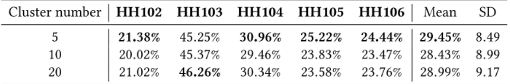
Table 4. Activity prediction accuracy of pre-clustered CSCRAFFT DBN on CASAS datasets.

Cluster number HH102 HH103 HH104 HH105 HH106 Mean SD 5 21.38% 45.25% 30.96% 25.22% 24.44% 29.45% 8.49 10 20.02% 45.37% 29.46% 23.83% 23.47% 28.43% 8.99 20 21.02% 46.26% 30.34% 23.58% 23.76% 28.99% 9.17

Markov property. However, we observed that the home and occupants monitored by the system have a great impact on this result. In particular, it seems that for some homes (such as in the HH102 dataset), the routine of the occupant is for the most part a Markov process. In other homes, the ideal non-Markovian depth to use for activity prediction can vary, although depths of 4 and more seem detrimental to prediction accuracy on the CASAS datasets. Therefore, estimating the optimal non-Markovian depth for a specific home is essential, and should be the focus of future work in activity prediction in homes.

4.4 Cognitive States-based Activity Prediction

We report in Table 4 the accuracy of the pre-clustered CSCRAFFT model on the CASAS datasets, where the cognitive state node is pre-labelled using the k-means clustering algorithm. We performed the experiments with 5, 10, and 20 clusters (i.e. possible states for the cognitive state node).

We observe that the pre-clustered CSCRAFFT DBN is approximately as accurate as the CRAFFT DBN, or even slightly worse than the CRAFFT DBN depending on the number of states. For a number of states of 10, the pre-clustered CSCRAFFT model is a full percent less accurate than the CRAFFT model (28.43% compared to 29.59%).

We report in Table 5 the best, worst, and average accuracies of the latent CSCRAFFT model with a number of cognitive states varying between 1 and 20. Much like for the NMCRAFFT model, we observe three different trends, depending on the dataset:

(1) Prediction accuracy is mostly unaffected by the latent cognitive state node. This trend is observed on HH104.

(2) Prediction accuracy of CSCRAFFT is on average better than CRAFFT. This trend is observed on HH102 and HH105.

(3) Prediction accuracy of CSCRAFFT is on average worse than CRAFFT. This trend is observed on HH103 and HH106.

However, we can note that the best configuration of CSCRAFFT (i.e. the right number of states) is always better than CRAFFT for each dataset (except for HH104 where they have identical accuracies).

Table 5. Activity prediction accuracy of CSCRAFFT DBN with unobserved latent nodes on CASAS datasets.

Model HH102 HH103 HH104 HH105 HH106 Mean SD Worst 21.38% 45.50% 30.87% 25.22% 23.67% 29.33% 8.67% Average 21.90% 45.99% 30.96% 25.49% 24.17% 29.70% 8.67% Best 22.47% 46.64% 30.96% 25.73% 24.73% 30.11% 8.72%

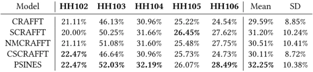
Table 6. Activity prediction accuracy of PSINES DBN and others DBNs in their best configurations on CASAS datasets. Model HH102 HH103 HH104 HH105 HH106 Mean SD CRAFFT 21.11% 46.13% 30.96% 25.22% 24.54% 29.59% 8.85% SCRAFFT 20.00% 50.25% 31.66% 26.45% 27.62% 31.20% 10.24% NMCRAFFT 21.11% 51.08% 31.60% 25.48% 27.75% 30.51% 10.41% CSCRAFFT 22.47% 46.64% 30.96% 25.73% 24.73% 30.11% 8.72% PSINES 22.47% 52.03% 32.19% 26.07% 28.49% 32.25% 10.38%

4.5 PSINES: A Combined Model for Activity Prediction

We report in Table 6 the prediction accuracy of the combined PSINES DBN on the CASAS datasets. This final set of experiments shows that combining all 3 improvements (sensor aggregate nodes, non-Markovianness, and cognitive state nodes) into one model leads on average to a model that is more accurate than any other DBN predictor we have tested. For example, PSINES reaches a prediction accuracy of 52.03% on HH103, which is almost 1% higher than the accuracy of the second best DBN (3-NMCRAFFT with 51.08%), and nearly 6% higher than the initial CRAFFT DBN of Nazerfard and Cook (46.13%). PSINES performs worse than another tested DBN only on HH105 in our experiments, where it still comes second after SCRAFFT (26.07% against 26.45%).

We also applied the PSINES DBN to the Orange4Home dataset, using the first 2 weeks of data as a training set, the third week as validation set, and the last week as the test set. We present the results of this experiment in Table 7. PSINES reaches on this dataset a prediction accuracy of 89.52%. CRAFFT, on the other hand, only reaches an accuracy of 61.68%, which is substantially less. The main improvements in prediction accuracy on this dataset come from the inclusion of non-Markovian previous activities. Indeed, 2-NMCRAFFT and 3-NMCRAFFT obtain prediction accuracies of 87.74% and 88.57% respectively, which is close to the performance of the full PSINES model. On the other hand, the inclusion of cognitive state nodes through CSCRAFFT only marginally improves accuracy: CSCRAFFT with 6 states reaches a prediction accuracy of 63.55%.

We have also compared PSINES to a predictive Long Short-Term Memory (LSTM) neural network, which are very popular prediction models that have allowed great progress in recent years in difficult areas of research such as natural language processing [31]. We used the following hyperparameter configuration for training: learning rate of 0.01, 300 epochs, 1 LSTM layer with 20 hidden neurons, and a weight decay of 0.0001. We averaged the accuracy over 5 repetitions, using the same protocol (2 first weeks for training, third week for validation, and fourth week for testing) as for PSINES. Note that DBN training does not involve randomness (whereas neural networks do, in particular the initial weights), so the accuracies obtained are always the same (hence why we did no averaging over repetitions). We see that PSINES is significantly more accurate than the LSTM, with an accuracy of 89.52% compared to 80.56% ± 2.77%.

Table 7. Activity prediction accuracy on the Or-ange4Home dataset. Model Accuracy CRAFFT 61.68% 2-NMCRAFFT 87.74% 3-NMCRAFFT 88.57% CSCRAFFT 63.55% PSINES 89.52% LSTM 80.56% ± 2.77%

Table 8. Availability prediction accuracy on the Orange4Home dataset. Model Accuracy CRAFFT 72.90% 2-NMCRAFFT 82.08% 3-NMCRAFFT 81.90% CSCRAFFT 75.70% PSINES 82.08% LSTM 78.68% ± 2.28%

One of the possible reasons for these results is the fact that LSTM and other neural architectures (like CNNs) require large amounts of labelled data for proper generalization; however, obtaining labelled data of activities at home is precisely one of the major difficulties in this research topic [32]. Therefore, it seems that our PSINES model, based on a DBN, has better generalization properties when using few training examples, compared to more popular neural models such as an LSTM. PSINES is thus better suited for smart home situations where having a low number of labelled examples is common.

The importance of introducing non-Markovianness to the prediction model can be easily il-lustrated in the Orange4Home dataset. Let us take the example of the activity “Going up” in the Staircase. If we only use this activity as well as related context information of place, hour of the day, day of the week, as in CRAFFT, it is obviously very difficult to predict what the occupant will do because multiple rooms can be reached and thus multiple activities can be performed once the user changed floor (although hour of the day and day of the week might give some hints as to why the occupant was going upstairs). On the other hand, if the predictor knows the previous 2 or 3 activities that the occupant was doing before going upstairs, it will most likely have an easier time identifying a part of the routine of the occupant and thus predict accurately their next activity. Most confusions thus occur when the occupant abruptly changes their routine in an unexpected manner. For example, PSINES incorrectly predicts that the occupant will perform “Preparing” in the Kitchen on Tuesday 21, 2017, when in fact the occupant decided to leave the home to have lunch. In another example, PSINES predicts twice, on Tuesday 21, 2017 and Wednesday 22, 2017, that the occupant will be “Watching TV” in the Office at the end of the day, when they in fact will be “Going down” because they decided to skip watching TV. In both of those examples, these changes in routine had never occurred before in the training set, and thus could not be learned by PSINES.

All in all, we see that using PSINES, we obtain a predictor that reaches fairly acceptable prediction accuracy on the Orange4Home dataset. Context-aware services that require predicted information would not be implementable if we were using the standard CRAFFT approach, which does not predict activities sufficiently accurately.

4.6 PSINES: Extension for Availability Prediction

We used, on the Orange4Home dataset, availability values provided by the inhabitant during 4 weeks. The first two weeks are used for learning our model, the third week for validating our hyper-parameters and the last week for testing. This experiment is done one time, due a lack of available data. Availability can take one of 5 values:

• 0: not available for anyone • 1: no decision / not sure

• 2: available for relatives

• 3: available for relatives and colleagues • 4: available for anyone

We report in Table 8 the availability prediction accuracy of the combined PSINES DBN on the Orange4Home dataset in comparison to other DBN architectures with the relative best configuration. This extended set of experiments shows that PSINES reaches an availability prediction accuracy of 82.08%, which is almost 10% higher than the accuracy of CRAFFT with availability nodes (72.90%). We observe also that modelling cognitive states with CSCRAFFT improves the original CRAFFT architecture. In this experiment, 2-NMCRAFFT slightly outperforms 3-NMCRAFFT, unlike in the previous activity prediction experiment, presented in Table 7. Nevertheless, the difference is not very significative. We have also tested an LSTM for availability prediction, using the same configuration as for activity prediction. Once again, we see that the LSTM is less accurate than PSINES (78.68% ± 2.28% compared to 82.08%). PSINES is overall the most accurate availability prediction model in these experiments (along with 2-NMCRAFFT). Therefore, PSINES can predict activity and availability simultaneously with the highest level of accuracies of all tested models.

5 CONCLUSIONS AND PERSPECTIVES

We presented in this paper a new activity and availability prediction model, called PSINES, in an autonomous and adaptive system. We experimentally evaluated activity prediction, as well as intermediary contributions, on 5 datasets of the literature. We showed that each partial contribution can improve prediction accuracy, and that PSINES is the most accurate model we tested on these CASAS datasets, on average. We obtained similar results on the Orange4Home dataset for activity prediction and successfully extended our approach for availability prediction.

First, we showed that sensor data can be valuable for activity prediction, in addition to context data. These findings may influence the choice of sensor installations and prediction algorithms used in smart home systems that require activity prediction capabilities.

Second, we also showed that routines of daily living do not, generally, respect the first-order Markov property. As such, predictors that inherently are first-order Markov models (such as the original CRAFFT model) will be limited in their prediction capabilities. Non-Markov models exhibit, in our experiments, significantly more accurate prediction performances.

Third, we showed that the introduction of a latent node, meant to represent the cognitive state of the occupant, can lead to slightly more accurate models. However, improvements are smaller than the other two contributions, and modelling (such as the optimal number of cognitive state classes) seems difficult. Further work is required to investigate the effects of introducing such latent nodes in DBN-based activity prediction models in smart homes.

Finally, we showed that the combination of these 3 contributions, PSINES, is the most accurate model we have studied for activity prediction in homes, according to our experiments. Ultimately, we saw that each specific dataset (and therefore, each specific home) requires a specific prediction model. Indeed, we have seen in our experiments that each of our contributions has significantly varying effects on activity prediction, due to the variety of different occupant behaviours and home environments. Therefore, we suggest that smart home systems which require activity prediction capabilities must construct their own prediction model independently of other homes, and not use a generic model that would be applied to any home.

Predicting next activities and inhabitant availabilities is a necessary step to provide new and helpful context-aware services in homes. High prediction accuracy is essential so as to limit the inappropriate behaviours. Our contributions to the problem of activity prediction are thus valuable for this purpose, although further work is still required to reach greater prediction accuracies.

While activity prediction accuracy, despite our contributions, was still relatively low on the CASAS datasets, it can be considered acceptable on Orange4Home (89.52%). The results on Or-ange4Home (82.08%) for forecasting inhabitant availability are also very promising.

Acknowledgments.We thank Paul Compagnon for his help on LSTM experiments. REFERENCES

[1] James L. Crowley and Joelle Coutaz. 2015. An ecological view of smart home technologies. In European Conference on Ambient Intelligence. Springer, 1–16.

[2] Shaoen Wu, Jacob B. Rendall, Matthew J. Smith, Shangyu Zhu, Junhong Xu, Honggang Wang, Qing Yang, and Pinle Qin. 2017. Survey on prediction algorithms in smart homes. IEEE Internet of Things Journal, 4, 3, 636–644.

[3] Claude Elwood Shannon. 1948. A mathematical theory of communication. Bell Syst. Tech. J., 27, 623–656.

[4] Rakesh Agrawal and Ramakrishnan Srikant. 1994. Fast algorithms for mining association rules in large databases. In Proceedings of the 20th International Conference on Very Large Data Bases. Morgan Kaufmann Publishers Inc., 487–499.

[5] Heikki Mannila, Hannu Toivonen, and A. Inkeri Verkamo. 1997. Discovery of frequent episodes in event sequences. Data mining and knowledge discovery, 1, 3, 259–289.

[6] Jiawei Han, Jian Pei, and Yiwen Yin. 2000. Mining frequent patterns without candidate generation. In ACM sigmod record number 2. Volume 29. ACM, 1–12.

[7] M. J. Zaki, S. Parthasarathy, M. Ogihara, and W. Li. 1997. New algorithms for fast discovery of association rules. In Proceedings of the Third International Conference on Knowledge Discovery and Data Mining. AAAI Press, 283–286.

[8] Karthik Gopalratnam and Diane J. Cook. 2007. Online sequential prediction via incremental parsing: the active leZi algorithm. IEEE Intelligent Systems, 1, 52–58.

[9] Amiya Bhattacharya and Sajal K. Das. 2002. Lezi-update: an information-theoretic framework for personal mobility tracking in pcs networks. Wireless Networks, 8, 2-3, 121–135.

[10] Muhammad Raisul Alam, Mamun Bin Ibne Reaz, and M. A. Mohd Ali. 2012. SPEED: an inhabitant activity prediction algorithm for smart homes. IEEE Transactions on Systems, Man, and Cybernetics-Part A: Systems and Humans, 42, 4, 985–990.

[11] Piotr Augustyniak and Grażyna Ślusarczyk. 2018. Graph-based representation of behavior in detection and prediction of daily living activities. Computers in biology and medicine, 95, 261–270.

[12] Sawsan Mahmoud, Ahmad Lotfi, and Caroline Langensiepen. 2013. Behavioural pattern identification and prediction in intelligent environments. Applied Soft Computing, 13, 4, 1813–1822.

[13] Henry Kautz, Oren Etzioni, Dieter Fox, and Dan Weld. 2003. Foundations of assisted cognition systems.

[14] Dorothy N Monekosso and Paolo Remagnino. 2009. Anomalous behavior detection: support-ing independent livsupport-ing.

[15] Han Saem Park and Sung Bae Cho. 2010. Predicting user activities in the sequence of mobile context for ambient intelligence environment using dynamic bayesian network. In 2nd International Conference on Agents and Artificial Intelligence, ICAART 2010.

[16] Jihang Ye, Zhe Zhu, and Hong Cheng. 2013. What’s your next move: user activity prediction in location-based social networks. In Proceedings of the 2013 SIAM International Conference on Data Mining. SIAM, 171–179.

[17] Ashesh Jain, Avi Singh, Hema S Koppula, Shane Soh, and Ashutosh Saxena. 2016. Recurrent neural networks for driver activity anticipation via sensory-fusion architecture. In Robotics and Automation (ICRA), 2016 IEEE International Conference on. IEEE, 3118–3125.

[18] Sungjoon Choi, Eunwoo Kim, and Songhwai Oh. 2013. Human behavior prediction for smart homes using deep learning. In RO-MAN. Volume 2013, 173.

[19] Younggi Kim, Jihoon An, Minseok Lee, and Younghee Lee. 2017. An activity-embedding approach for next-activity prediction in a multi-user smart space. In Smart Computing (SMARTCOMP), 2017 IEEE International Conference on. IEEE, 1–6.

[20] Iram Fatima, Muhammad Fahim, Young-Koo Lee, and Sungyoung Lee. 2013. A unified framework for activity recognition-based behavior analysis and action prediction in smart homes. Sensors, 13, 2, 2682–2699.

[21] Abdulsalam Yassine, Shailendra Singh, and Atif Alamri. 2017. Mining human activity patterns from smart home big data for health care applications. IEEE Access, 5, 13131–13141. [22] Shailendra Singh, Abdulsalam Yassine, and Shervin Shirmohammadi. 2016. Incremental

mining of frequent power consumption patterns from smart meters big data. In Electrical Power and Energy Conference (EPEC), 2016 IEEE. IEEE, 1–6.

[23] Ehsan Nazerfard and Diane J. Cook. 2015. CRAFFT: an activity prediction model based on bayesian networks. Journal of ambient intelligence and humanized computing, 6, 2, 193–205. [24] Yoshinao Takemae, Takehiko Ohno, Ikuo Yoda, and Shinji Ozawa. 2006. Estimating human interruptibility in the home for remote communication. In CHI’06 Extended Abstracts on Human Factors in Computing Systems. ACM, 1397–1402.

[25] Kristine S. Nagel, James M. Hudson, and Gregory D. Abowd. 2004. Predictors of availability in home life context-mediated communication. In Proceedings of the 2004 ACM conference on Computer supported cooperative work. ACM, 497–506.

[26] Chien-Ming Huang and Bilge Mutlu. 2014. Learning-based modeling of multimodal behaviors for humanlike robots. In Proceedings of the 2014 ACM/IEEE international conference on Human-robot interaction. ACM, 57–64.

[27] Jina Lee, Stacy Marsella, David Traum, Jonathan Gratch, and Brent Lance. 2007. The rickel gaze model: a window on the mind of a virtual human. In International Workshop on Intelligent Virtual Agents. Springer, 296–303.

[28] Alaeddine Mihoub and Grégoire Lefebvre. 2018. Wearables and social signal processing for smarter public presentations. Transactions on Interactive Intelligent Systems.

[29] Diane J Cook, Aaron S Crandall, Brian L Thomas, and Narayanan C Krishnan. 2013. CASAS: a smart home in a box. Computer, 46, 7, 62–69.

[30] Julien Cumin, Grégoire Lefebvre, Fano Ramparany, and James L Crowley. 2017. A dataset of routine daily activities in an instrumented home. In International Conference on Ubiquitous Computing and Ambient Intelligence. Springer, 413–425.

[31] Klaus Greff, Rupesh K Srivastava, Jan Koutník, Bas R Steunebrink, and Jürgen Schmidhuber. 2016. LSTM: a search space odyssey. IEEE transactions on neural networks and learning systems, 28, 10, 2222–2232.

[32] Julien Cumin, Grégoire Lefebvre, Fano Ramparany, and James L. Crowley. 2017. Human activity recognition using place-based decision fusion in smart homes. In International and Interdisciplinary Conference on Modeling and Using Context. Springer, 137–150.