Coupled dictionary learning for unsupervised change detection between multimodal remote sensing images

HAL Id: hal-02397250

https://hal.archives-ouvertes.fr/hal-02397250

Submitted on 6 Dec 2019

HAL is a multi-disciplinary open access

archive for the deposit and dissemination of

sci-entific research documents, whether they are

pub-lished or not. The documents may come from

teaching and research institutions in France or

abroad, or from public or private research centers.

L’archive ouverte pluridisciplinaire HAL, est

destinée au dépôt et à la diffusion de documents

scientifiques de niveau recherche, publiés ou non,

émanant des établissements d’enseignement et de

recherche français ou étrangers, des laboratoires

publics ou privés.

Coupled dictionary learning for unsupervised change

detection between multimodal remote sensing images

Vinicius Ferraris, Nicolas Dobigeon, Yanna Cruz Cavalcanti, Thomas Oberlin,

Marie Chabert

To cite this version:

Vinicius Ferraris, Nicolas Dobigeon, Yanna Cruz Cavalcanti, Thomas Oberlin, Marie Chabert.

Coupled dictionary learning for unsupervised change detection between multimodal remote

sensing images.

Computer Vision and Image Understanding, Elsevier, 2019, 189, pp.1-15.

Any correspondence concerning this service should be sent

to the repository administrator: tech-oatao@listes-diff.inp-toulouse.fr

This is an author’s version published in:

http://oatao.univ-toulouse.fr/25034

To cite this version: Ferraris, Vinicius and Dobigeon,

Nicolas and Cruz Cavalcanti, Yanna and Oberlin, Thomas and

Chabert, Marie Coupled dictionary learning for unsupervised

change detection between multimodal remote sensing images.

(2019) Computer Vision and Image Understanding, 189. 1-15.

ISSN 1077-3142

Official URL

DOI : https://doi.org/10.1016/j.cviu.2019.102817

Open Archive Toulouse Archive Ouverte

OATAO is an open access repository that collects the work of Toulouse

researchers and makes it freely available over the web where possible

Coupled

_{dictionary learning for unsupervised change detection}

between

_{multimodal remote sensing images}

✩

,

✩✩

Vinicius

Ferraris

_,

_{Nicolas Dobigeon, Yanna Cavalcanti, Thomas Oberlin, Marie Chabert}

University of Toulouse, IRIT/INP-ENSEEEIHT, 2 Rue Camichel, 31071 Toulouse, France

Keywords:

Change detection Coupled dictionary learning Multimodality

Optical images SAR image

A B S T R A C T

Archetypal scenarios for change detection generally consider two images acquired through sensors of the same modality. However, in some specific cases such as emergency situations, the only images available may be those acquired through sensors of different modalities. This paper addresses the problem of unsupervisedly detecting changes between two observed images acquired by sensors of different modalities with possibly different resolutions. These sensor dissimilarities introduce additional issues in the context of operational change detection that are not addressed by most of the classical methods. This paper introduces a novel framework to effectively exploit the available information by modeling the two observed images as a sparse linear combination of atoms belonging to a pair of coupled overcomplete dictionaries learnt from each observed image. As they cover the same geographical location, codes are expected to be globally similar, except for possible changes in sparse spatial locations. Thus, the change detection task is envisioned through a dual code estimation which enforces spatial sparsity in the difference between the estimated codes associated with each image. This problem is formulated as an inverse problem which is iteratively solved using an efficient proximal alternating minimization algorithm accounting for nonsmooth and nonconvex functions. The proposed method is applied to real images with simulated yet realistic and real changes. A comparison with state-of-the-art change detection methods evidences the accuracy of the proposed strategy.

1. Introduction

Ecosystems exhibit permanent variations at different temporal and spatial scales caused by natural, anthropogenic, or even both fac-tors (Coppin et al.,2004). Monitoring spatial variations over a period of time is an important source of knowledge that helps understanding the possible transformations occurring on Earth’s surface. Therefore, due to the importance of quantifying these transformations, change detection (CD) has been an ubiquitous issue addressed in the remote sensing and geoscience literature (Lu et al.,2004).

Remote sensing CD methods can be first classified with respect to (w.r.t.) their supervision (Bovolo and Bruzzone,2007), depending on the availability of prior knowledge about the expected changes. More precisely, supervised CD methods require ground reference information about at least one of the observations. Conversely, unsupervised CD can be contextualized as automatic detection of changes without the need for any further external knowledge. Each class of CD methods present particular competitive advantages w.r.t. the others. For instance, su-pervised CD methods generally achieve better accuracy for predefined

✩ Part of this work has been supported by Coordenação de Aperfeiçoamento de Pessoal de Nível Superior (CAPES), Brazil, the EU FP7 through the ERANETMED JC-WATER program [MapInvPlnt Project ANR-15-NMED-0002-02] and the ANR, France-3IA Artificial and Natural Intelligence Toulouse Institute (ANITI). ✩✩ _{No author associated with this paper has disclosed any potential or pertinent conflicts which may be perceived to have impending conflict with this work.} For full disclosure statements refer tohttps://doi.org/10.1016/j.cviu.2019.102817.

∗ Corresponding author.

E-mail address: vinicius.ferraris@enseeiht.fr (V. Ferraris).

modalities whereas unsupervised methods are characterized by their flexibility and genericity. Nevertheless, implementing supervised meth-ods require the acquisition of relevant ground information, which is a very challenging and expensive task, in terms of human and time resources (Bovolo and Bruzzone,2007). Relaxing this constraints makes unsupervised methods more suitable for operational CD.

CD methods can also be categorized w.r.t. the imagery modalities the method is able to handle. As remote sensing encompasses many dif-ferent types of imagery modalities (e.g., single- and multi-band optical images, radar, LiDAR), dedicated CD methods have been specifically developed for each one by exploiting its acquisition process and the intrinsic characteristics of the resulting data. Thus, due to differences in the physical meaning and statistical properties of images from different sensor modalities, a general CD method able to handle all modalities is particularly difficult to design and to implement. For this reason, most of the CD methods focus on a pair of images from one single target modality. In this case, the images are generally compared pixel-wisely using the underlying assumption of same spatial resolutions (Singh,

1989; Bovolo and Bruzzone, 2015). Nevertheless, in some practical sce-narios such as, e.g., emergency missions due to natural disasters, when the availability of data and the responsiveness are strong constraints, CD methods may have to handle observations of different modalities and/or resolutions. This highlights the need for robust and flexible CD techniques able to deal with this kind of observations.

The literature about multimodal CD is very limited, yet a few rele-vant references include the works by Kawamura(1971),Bruzzone et al. (1999),Inglada(2002),Lu et al. (2004),Alberga et al. (2007),Mercier et al. (2008) and Prendes et al. (2015). However, multimodal CD has always been an important topic since the initial development of CD methods. Earlier work by Kawamura (1971) described the potential of CD between a multimodal collection of datasets (e.g., photographic, infrared and radar), applied to weather prediction and land surveil-lance. Three features are extracted from the pair and the CD algorithm is trained on a learning set. According to Lu et al. (2004), various methods dedicated to CD between images from different sources of data are grouped as geographical information system-based methods. For instance, Solberg et al. (1996) proposed a supervised classifica-tion of multisource satellite images using Markov random fields. The work of Bruzzone et al. (1999) uses compound classification to detect changes in multisource data. The method uses artificial neural networks to estimate the posterior probability of classes. Moreover, Inglada (2002) studies the relevance of several similarity measures between multisensor data. These measures are implemented in a CD context ( Al-berga et al., 2007). A preprocessing technique based on conditional copula that contributes to better statistically modeling multisensor images was proposed by Mercier et al. (2008). Besides, Brunner et al. (2010) presented a strategy to assess building damages using a pair of very high resolution (VHR) optical and radar images by geomet-rically modeling buildings in both modalities. Chabert et al. (2010) updated information databases by means of logistic regression. More recently, the work of Prendes et al. (2015) presented a supervised method to infer changes after learning a manifold defined by pairs of patches extracted from the two images. Although some of these methods present relatively high detection performance, they are often restrained to a specific modality or to a specific target application. For instance, Solano-Correa et al. (2018) proposed an approach to detect changes between multispectral images with different spatial and spectral resolutions by homogenization of radiometric and geometric image properties. However, this approach relies in particular on a tax-onomy of possible radiometric changes observed in very high resolution images. Moreover, some methods are only suitable for building damage assessment taking benefit of their high-level modeling, but show a poor adaptability to other scenarios (Brunner et al., 2010; Chabert et al., 2010). The other ones estimate some metrics from unchanged trained samples, which prevents their application within a fully unsupervised context (Bruzzone et al., 1999; Prendes et al., 2015; Mercier et al., 2008).

Recently, an unsupervised multi-source CD method based on cou-pled dictionary learning was addressed by Gong et al. (2016). In the proposed methodology, the CD is based on the reconstruction error of patches approximated thanks to estimated coupled dictionary and independent sparse codes. Atoms of the dictionary are learnt from pairs of patches jointly extracted from the observed images. Following the same principle, in Lu et al. (2017), a semi-supervised method was used to handle multispectral images based on joint dictionary learning. Both methods rely on the rationale that the coupled dictio-nary estimated from the observed images tends to produce stronger reconstruction errors in change regions rather than in unchanged ones. Because of the multi-modality, the problem has not been formulated in the image space, but rather in a latent space formed by the coupled dictionary atoms. However, both methods exhibit some crucial issues that may impair their relative performance. First, the underlying opti-mization problem is highly nonconvex and no convergence guarantees are ensured, even by using some traditional dictionary learning meth-ods (Aharon et al.,2006). Then, the considered CD problem has been

split into two distinct steps: dictionary learning and code estimation. The errors in code estimation may produce false alarms in the final CD even with reliable dictionary estimates. Also, the statistical model of the noise – inherent to each sensor modality – has not been taken into consideration explicitly, which may dramatically impact the CD performance (Campbell and Wynne,2011). Finally, these methods do not consider overlapping patches, which potentially would increase their robustness and thus do not explicitly handle the problem of possible differences in spatial resolutions (Ferraris et al., 2017b,a). The adequacy between the size of patches and the image scale is not discussed, although it may have a negative impact on the dictionary coupling and thus on the detection performance.

Overcoming these limitations, this paper proposes a similar method-ology to learn coupled dictionaries able to conveniently model multi-modal remote sensing images. Specifically, contrary to the aforemen-tioned methods, the problem is fully formulated without splitting the learning and coding steps. Also, an appropriate statistical model is derived to describe the image from each specific remote sensing modal-ity. Besides, the proposed method explicitly allows patch overlapping within the overall estimation process. To couple images with different resolutions, additional scaling matrices inspired by the work by Se-ichepine et al.(2014) are jointly estimated within the whole process. Finally, as the problem is highly nonconvex, it is iteratively solved based on the proximal alternating linearized minimization (PALM) algorithm (Bolte et al., 2014), which ensures convergence towards a critical point for some nonconvex nonsmooth problems. Note that the proposed patch-based method departs from segmentation-based methods which generally extract change information at an object-level, whose resolution is implicitly defined by the chosen segmentation procedure (Feng et al.,2018). Instead, the proposed method linearly decomposes overlapping square patches onto an appropriate common latent space, which allows CD to be operated at a pixel level.

This manuscript is organized as follows. Generic and well-admitted image models are introduced in Section2. Capitalizing on these image models, Section3formulated the CD problem as a coupled dictionary learning. Section4proposes an algorithmic solution to minimize the resulting CD-based objective function. Section5reports experimental results obtained on synthetic images, considering three distinct simula-tion scenarios. Experiments conducted on real images are presented in Section5.3. Finally, Section6concludes the manuscript.

2. Image models

2.1. Forward model

Let us consider that the image formation process inherent to all digital remote sensing imagery modalities is modeled as a sequence of transformations, denoted 𝑇 [⋅]. This sequence applies to the original scene to produce the sensor output image. This output image is referred to as the observed image and is denoted by 𝐘 ∈ R𝐿×𝑁 _{consisting of}

𝑁 voxels 𝐲𝑖 ∈ R𝐿 stacked lexicographically that is from left to right, row by row. The voxel dimension 𝐿 may represent different quantities depending on the modality of the data. For instance, it stands for the number of spectral bands in the case of multiband optical images ( Fer-raris et al., 2017b) or for the number of polarization modes in the case of polarimetric synthetic aperture radar (POLSAR) images. The observed image provides a limited representation of the original scene with properties imposed by the image signal processor characterizing the sensor. The original scene cannot be exactly represented because of its continuous nature, but it can be conveniently approximated by a latent (i.e., unobserved) image 𝐗 ∈ R𝐿×𝑁_{related to the observed image} as follows

𝐘= 𝑇 [𝐗]. (1)

The sequence of transformations 𝑇 [⋅] operated by the sensor over the latent image is often referred to as the degradation process. It may

represent resolution degradations accounting for the spatial and/or spectral characteristics of the sensor (Ferraris et al.,2017a,b). In this paper, it specifically models the intrinsic noise corruption associated to the sensor modality (Sun and Févotte,2014). The latent image 𝐗 can be understood, in this context, as a noise-free version of the observed image 𝐘 with the same resolution.

More precisely, the transformation 𝑇 [⋅] underlies the likelihood function 𝑝(𝐘|𝐗) which statistically models the observed image 𝐘 condi-tionally to the latent image 𝐗 by taking into account the noise statistics. The noise statistical model mainly depends on the modality and rely on some classical distributions, e.g., the Gaussian distribution for optical images or the Gamma distribution for multi-look SAR images. More-over, as already pointed out by Févotte et al. (2009) in a different application context, for a wide family of distributions, this likelihood function relies on a divergence measure (⋅|⋅) between the observed and latent images, which finally defines an explicit data-fitting term through a negative-log transformation

− log 𝑝(𝐘|𝐗) = 𝜙−1(𝐘|𝐗) + 𝜃 (2) where 𝜙 and 𝜃 are parameters characterizing the distributions. In Appendix A, the divergence measures (⋅|⋅) are derived for two of the most common remote sensing image modalities, namely optical multiband and SAR images, considered in this work.

2.2. Latent image sparse model

Sparse representations have been an ubiquitous and well-admitted tool to model images in various applications and task-driven con-texts (Mairal,2014). Indeed, natural images are known to be compress-ible in a transformed domain, i.e., they can be efficiently represented by a few expansion coefficients acting on basis functions (Mallat, 2009). This finding has motivated numerous works on image under-standing, compression and denoising (Olshausen and Field,1997;Chen et al.,2001). In earlier works, this transformed domain, equivalently defined by the associated basis functions, was generally fixed in ad-vance and chosen in agreement with the expected spatial content of the images (Mallat, 2009). Thus, the basis functions belonged to pre-determined families with specific representation abilities, such as cosines, wavelets, contourlets, shearlets, among others. More recently, the seminal contribution by Aharon et al. proposed a new paradigm by learning an overcomplete dictionary jointly with a sparse code (Aharon et al., 2006). This dictionary learning-based approach exploits the key property of self-similarity characterizing the images to provide an adaptive representation. Indeed, it aims at identifying elementary patches that can be linearly and sparsely combined to approximate the observed image patches. In this paper, following the approach byAharon et al.(2006), we propose to resort to this dictionary-based representation to model the latent image 𝐗. More precisely, the image is first decomposed into a set of 𝑁p 3D-patches with 1 ≤ 𝑁p≤ 𝑁. Let _𝑖∶ R𝐿×𝑁_→

R𝐾2𝐿denote a binary operation modeling the extraction, from the image, of the 𝑖th patch (𝑖 ∈ {1, … , 𝑁p}) such that

𝐩𝑖= 𝑖𝐗 (3)

where 𝐩𝑖∈ R𝐾 2_𝐿

stands for the 𝑖th 𝐾 ×𝐾 ×𝐿-pixel patch in its vectorized form. The integer 𝐾 > 1 defines the spatial size of the patches, i.e., its number of rows and columns before being vectorized. Note that the number of patches 𝑁p is such that 1 ≤ 𝑁p ≤ 𝑁 and patches may overlap. The choice of the number 𝑁_pof patches will be more deeply discussed in Section3in the specific context of CD. The conjugate of the patch-extraction operator,1 _{denoted }𝑇

𝑖, acts on 𝐩𝑖 to produce a zero-padded image composed by the unique patch 𝐩𝑖located at the 𝑖th spatial position.

1 _{Note that, despite a slight abuse of notation, the operator  (resp., }𝑇₎

does not stand for a matrix, but rather for a linear operator acting on the image 𝐗 (resp., the patch 𝐩𝑖) directly.

In accordance with dictionary-based representation principles, these patches are assumed to be approximately and independently mod-eled as sparse combinations of atoms belonging to an overcomplete dictionary 𝐃 =[𝐝1,… , 𝐝𝑁d ] ∈ R𝐾2_𝐿×𝑁 d 𝐩𝑖|𝐃, 𝐚𝑖∼  ( 𝐃𝐚𝑖, 𝜎2𝐈𝑁d ) (4) where 𝑁d>0stands for the user-defined number of atoms composing the dictionary, commonly referred to as dictionary size and 𝐚𝑖 ∈ R𝑁d represents the code (coefficients) of the current patch over the

dictionary, 𝜮 = 𝜎2_𝐈

𝑁d is the error covariance matrix and . Let 𝐏 ∈

R𝐾2𝐿×𝑁p ₌ [_𝐩 1,… , 𝐩𝑁p

]

denote the matrix that stacks the set of all, possibly overlapping, patches extracted from the latent image 𝐗 at

𝑁p spatial positions arranged on a generally regular spatial grid and enumerated in a lexicographical order (i.e., from left to right and top to bottom of the image). The matrix 𝐀 ∈ R𝑁d×𝑁p ₌

[

𝐚1,… , 𝐚𝑁p

] is the code matrix in which each column represents the code for each corresponding column of 𝐏. The overcompleteness property of the dictionary, occurring when the number of atoms is greater than the effective dimensionality of the input space, 𝑁d ≫ 𝐾2𝐿, allows for the sparsity of the representation (Olshausen and Field, 1997). The overcompleteness implies redundancy and non-orthogonality between atoms. This property is not necessary for the decomposition, but has been proved to be very useful in some applications like denoising and compression (Aharon et al., 2006). Given the image patch matrix 𝐏, dictionary learning aims at recovering the set of atoms 𝐃 and the associated code matrix 𝐀 and it is generally tackled through a 2-step procedure. First, inferring the code matrix 𝐀 associated with the patch matrix 𝐏 and the dictionary 𝐃 can be formulated as a set of 𝑁p sparsity-penalized optimization problems. Sparsity of the code vectors

𝐚𝑖 = [

𝑎1𝑖,… , 𝑎𝑁d𝑖

]𝑇

(𝑖 = 1, … , 𝑁p) can be promoted by minimizing its 𝓁₀-norm. However, since this leads to a non-convex problem (Chen et al.,2001), it is generally substituted by the corresponding convex relaxation, i.e., an 𝓁1-norm. Within a probabilistic framework, taking into account the expected non-negativeness of the code, this choice can be formulated by assigning a single-side exponential (i.e., Laplacian) prior distribution to the code components, assumed to be a priori independent 𝐚𝑖∼ 𝑁d ∏ 𝑗=1 (𝑎𝑗𝑖; 𝜆) (5)

where 𝜆 is the hyperparameter adjusting the sparsity level over the code. Conversely, learning the dictionary 𝐃 given the code 𝐀 can also be formulated as an optimization problem. As the number of solutions for the dictionary learning problem can be extremely large, one common assumption is to constrain the energy of each atom, thereby preventing 𝐃 to become arbitrarily large (Mairal et al.,2009). Moreover, in the particular context considered in this work, to pro-mote the positivity of the reconstructed patches, the atoms are also constrained to positive values. Thus, each atom will be constrained to the set  ≜ { 𝐃∈ R𝐾2𝐿×𝑁d + ∣ ∀𝑗 ∈ { 1, … , 𝑁d,} ‖‖‖𝐝𝑗‖‖_‖ 2 2= 1 } . (6) 2.3. Optimization problem

Adopting a Bayesian probabilistic formulation of the image model introduced in Sections2.1 and 2.2, the posterior probability of the unknown variables 𝐗, 𝐃 and 𝐀 can be derived using the probability chain rule (Gelman,2004)

𝑝(𝐗, 𝐃, 𝐀|𝐘) ∝ 𝑝(𝐘|𝐗)𝑝(𝐗|𝐃, 𝐀)𝑝(𝐃)𝑝(𝐀) (7) where 𝑝(𝐘|𝐗) is the likelihood function relating the observation data to the latent image through the direct model (1), 𝑝(𝐗|𝐃, 𝐀) is the dictionary-based prior model of the latent image, 𝑝(𝐃) and 𝑝(𝐀) are

MAP estimator _𝐗̂

MAP, ̂𝐃MAP, ̂𝐀MAP

the (hyper-)prior distributions associated with the dictionary and the sparse code. Under_{{ a maximum a }}posteriori (MAP) paradigm, the joint

can be derived by minimizing the negative log-posterior, leading to the following minimization problem

{

̂

𝐗MAP, ̂𝐃MAP, ̂𝐀MAP } ∈ argmin_{𝐗,𝐃,𝐀} (𝐗, 𝐃, 𝐀) (8) with  (𝐗, 𝐃, 𝐀) = (𝐘|𝐗) + 𝜎 2 2 𝑁p ∑ 𝑖=1‖‖ 𝑖𝐗− 𝐃𝐚𝑖‖‖ 2 F+ + 𝜆‖𝐀‖₁+ 𝜄(𝐃) (9)

where 𝜄represents the indicator function on the set ,

𝜄(𝑧) = {

0 if 𝑧 ∈ 

+∞ elsewhere (10)

and (⋅|⋅) is the data-fitting term associated with the image modality. This model has been widely advocated in the literature, e.g., for denoising images of various modalities (Elad and Aharon, 2006;Ma et al.,2013). Particularly, inMa et al.(2013), an additional regulariza-tion 𝛹 (𝐗) of the latent image was introduced as the target modalities may present strong fluctuations due to their inherent image formation process, i.e. Poissonian or multiplicative gamma processes. The final objective function(9)can thus be rewritten as

 (𝐗, 𝐃, 𝐀) = (𝐘|𝐗) + 𝜎 2 2 𝑁p ∑ 𝑖=1‖‖ 𝑖𝐗− 𝐃𝐚𝑖‖‖ 2 F+ 𝛹 (𝐗) + 𝜆‖𝐀‖1+ 𝜄(𝐃) (11)

where, for instance, 𝛹 (𝐗) can stand for a total-variation (TV) regular-ization (Ma et al.,2013).

The next section expands the proposed image models to handle a pair of observed images in the specific context of CD.

3. From change detection to coupled dictionary learning

3.1. Problem statement

Let us consider two geographically aligned observed images 𝐘1 ∈ R𝐿1×𝑁1 and 𝐘_{2 ∈ R}𝐿2×𝑁2acquired by two sensors 𝖲₁ and 𝖲₂ at times

𝑡1and 𝑡2, respectively. The ordering of acquisition times is indifferent, i.e., either 𝑡2 < 𝑡1 or 𝑡2 > 𝑡1 are possible cases and the order does not impact the applicability the proposed method. The problem addressed in this paper consists in detecting significant changes between these two observed images. This is a challenging task mainly due to the possible dissimilarities in terms of spatial and/or spectral resolutions and of modality. Indeed, resolution dissimilarity prevents any use of classical CD algorithms without homogenization of the resolutions as a preprocessing step (Singh,1989;Bovolo and Bruzzone,2015). More-over modality dissimilarity, which makes most of the CD algorithms inoperative because their inability of handling images of different na-ture (Ferraris et al.,2017a,b). To alleviate this issue, this work proposes to improve and generalize the CD methods introduced bySeichepine et al. (2014), Gong et al. (2016), Lu et al. (2017). Following the widely admitted forward model described in Section2.1and adopting consistent notations, the observed images 𝐘₁ and 𝐘₂can be related to two latent images 𝐗1∈ R𝐿1×𝑁1and 𝐗2∈ R𝐿2×𝑁2

𝐘1= 𝑇1[𝐗1] (12a)

𝐘2= 𝑇2[𝐗2] (12b)

where 𝑇1 and 𝑇2 denote two degradation operators imposed by the sensors 𝖲1 and 𝖲2. Note that (12) is a double instance of the model (1). In particular, in the CD context considered in this work, the two

latent images 𝐗₁ and 𝐗₂ are supposed to represent the same geo-graphical region provided the observed images have been beforehand co-registered.

Both latent images can be represented thanks to a dedicated dictionary-based decomposition, as stated in Section2.2. More pre-cisely, a pair of homologous patches extracted from each image repre-sents the same geographical spot. Each patch can be reconstructed from a sparse linear combination of atoms of an image-dependent dictionary. In the absence of changes between the two observed images, the sparse codes associated with the corresponding latent image are expected to be approximately the same and the two learned dictionaries are coupled (Yang et al.,2010,2012; Zeyde et al.,2010). This coupling can be understood as the ability of deriving a joint representation for homologous multiple observations in a latent coupled space (Gong et al.,2016). Akin to the manifold proposed byPrendes et al.(2015), this representation offers the opportunity to analyze images of different modalities in a common dual space. In the case where a pair of homol-ogous patches has been extracted from two images representing the same scene, given perfect estimated coupled dictionaries, each patch should be exactly reconstructed thanks to the same sparse code. In other words, the pair of patches is an element of the latent coupled space. Nevertheless, in the case where the pair of homologous patches does not represent exactly the same scene, owing to a change that occurs between acquisitions, perfect reconstruction cannot be achieved using the same code. This means that the pair of patches does not belong to the coupled spaces. Using the same code for reconstruction amounts to estimate the point in the coupled spaces that best approximates the patch pair. Thereby, relaxing this constraint in some possible change locations may provide an accurate reconstruction of both images while spatially mapping change locations. In the specific context of CD addressed in this work, this finding suggests to evaluate any change between the two observed, or equivalently latent, images by comparing the corresponding codes

𝛥𝐀= 𝐀2− 𝐀1 (13)

where 𝛥𝐀 =[𝛥𝐚1,… , 𝛥𝐚𝑁_p ]

and 𝛥𝐚𝑖 ∈ R𝑁d denotes the code change vector associated with the 𝑖th patch, 𝑖= 1, … , 𝑁p. Then, to spatially locate the changes, a natural approach consists in monitoring the mag-nitude of 𝛥𝐀, summarized by the code change energy image (Bovolo and Bruzzone,2007) 𝐞=[𝑒1,… , 𝑒𝑁p ] ∈ R𝑁p ₍₁₄₎ with 𝑒𝑖= ‖‖𝛥𝐚𝑖‖‖2, 𝑖= 1, … , 𝑁p.

Note that, in the case of analyzing a pair of optical images,Zanetti et al. (2015) proposed to describe the components 𝑒𝑖of the energy vector

𝐞thanks to a Rayleigh–Rice mixture model whose parameters can be estimated to locate the changes. Conversely, in this work we propose to derive the CD rule directly from this magnitude. When the CD problem in the 𝑖th patch is formulated as the binary hypothesis testing

{

0,𝑖 ∶ no change occurs in the 𝑖th patch _1,𝑖 ∶ a change occurs in the 𝑖th patch

a patch-wise statistical test can be written by thresholding the code change energy

𝑒𝑖 _1,𝑖

≷

_0,𝑖𝜏

where the threshold 𝜏 ∈ [0, ∞] implicitly adjusts the target probability of false alarm or, reciprocally, the probability of detection. The final binary CD map denoted 𝐦 =[𝑚1,… , 𝑚𝑁_p

] ∈ {0, 1}𝑁p_{can be derived as} 𝑚𝑖= { 1 if 𝑒𝑖≥ 𝜏 (1,𝑖) 0 otherwise (0,𝑖).

ri by the observed image of highest resolution, i.e., 𝑁p= max

{

𝑁1, 𝑁2 The spatial resolution of this CD map is defined by the number 𝑁pof homologous patches extracted from the latent images 𝐗1 and 𝐗2. This number can be tailored by the user according to the adopted strategy of patch extraction. In practice, to reach the highest resolution, overlap-ping patches should be extracted according to the regular g d defined_} . Finally, to solve the multimodal image CD problem, the key issue lies in the joint estimation of the pair of representation codes{𝐀1, 𝐀2

} or, equivalently, to the joint estimation of one code matrix and of the change code matrix, i.e. of {𝐀1, 𝛥𝐀

}

, as well as of the pair of coupled dictionary {𝐃1, 𝐃2

} _{and consequently of the pair of latent} images{𝐗1, 𝐗2

}_{from the joint forward model(12). The next paragraph} introduces the CD-driven optimization problem to be solved.

3.2. Coupled dictionary learning for CD

The single dictionary estimation problem presented on Section2.3 can be generalized to take into account the modeling presented in Sec-tion3.1. Nevertheless, some previous considerations must be carefully handled in order to provide good coupling of the two dictionaries.

As the prior information about the dictionaries constrains each atom into the set  of unitary energy defined by(6), an unbiased estimation of the code change vector would allow a pair of unchanged homologous patches to be reconstructed with exactly the same code, while changed patches would exhibit differences in their code. Obviously, this can only be achieved if the coupled dictionaries represent data with the same dynamics and resolutions. However, when analyzing images of different modalities and/or resolutions, this assumption can be not fulfilled. To alleviate this issue, we propose to resort to the strategy proposed by Se-ichepine et al. (2014), by introducing an additional diagonal scaling matrix constrained to the set  ≜{𝐒∈ R𝑁d1×𝑁d1

+ ∣ 𝐒 = diag(𝐬), 𝐬 ⪰ 0 } where 𝑁d1is the size of the dictionary 𝐃1. This scaling matrix gathers the code energy differences originated from different modalities for each pair of coupled atoms. This is essential to ensure that the sparse codes of the two observed images are directly comparable, following (13), and then properly estimated. Therefore, considering a pair of homologous patches, their joint representation model derived from(4) can be written as 𝐩1𝑖= 1𝑖𝐗1≈ 𝐃1𝐒𝐚1𝑖 𝐩2𝑖= 2𝑖𝐗2≈ 𝐃2𝐚2𝑖= 𝐃2 ( 𝐚1𝑖+ 𝛥𝐚𝑖 ) (15) where{𝐩1𝑖, 𝐩2𝑖 }

represents the pair of homologous patches and 𝐒 is the diagonal scaling matrix.

Since the codes 𝐀1 and 𝐀2 are now element-wise comparable, a natural choice to enforce coupling between them should be the equality

𝐀1= 𝐀2= 𝐀. This has been a classical assumption in various coupled dictionary learning applications (Yang et al.,2010;Zeyde et al.,2010; Yang et al.,2012). Nevertheless, in a CD context, some spatial positions may not contain the same objects. To account for possible changes in some specific locations while most of the patches remain unchanged, as inFerraris et al.(2017b), the code change energy matrix 𝐞 defined by(14)is expected to be sparse. As a consequence, the corresponding regularizing function is chosen as the sparsity-inducing 𝓁1-norm of the code change energy matrix 𝐞 or, equivalently, as the 𝓁2,1-norm of the code change matrix

𝜙2(𝛥𝐀) =‖𝛥𝐀‖2,1= 𝑁p

∑ 𝑖=1‖‖𝛥𝐚

𝑖‖‖2. (16)

This regularization is a specific instance of the non-overlapping group-lasso penalization (Bach,2011) which has been considered in various applications to promote structured sparsity (Wright et al.,2009;Févotte and Dobigeon,2015;Ferraris et al.,2017b).

Then, a Bayesian model extending the one derived for a single image (7)leads to the posterior distribution of the parameters of interest

𝑝(𝐗1, 𝐗2, 𝐃1, 𝐃2, 𝐒, 𝐀1, 𝛥𝐀|𝐘1, 𝐘2 ) ∝ 𝑝(𝐘1|𝐗1)𝑝(𝐘2|𝐗2) × 𝑝(𝐗_1|𝐃1, 𝐒, 𝐀1)𝑝(𝐗2|𝐃2, 𝐀1, 𝛥𝐀) × 𝑝(𝐃1)𝑝(𝐃2)𝑝(𝐒)𝑝(𝐀1)𝑝(𝛥𝐀). (17)

By incorporating all previously defined prior distributions (or, equiva-lently, regularizations), the joint MAP estimator 𝜣̂

MAP = {

̂

𝐗_1,MAP, ̂𝐗_2,MAP, ̂𝐃_1,MAP, ̂𝐃_2,MAP, ̂𝐒_MAP, ̂𝐀_1,MAP, 𝛥 ̂𝐀_MAP}of the quantities of interest can be obtained by minimizing the negative log-posterior, leading to the following minimization problem

̂ 𝜣_{MAP∈ argmin𝜣 (𝜣) (18)} with  (𝜣) ≜ (𝐗1, 𝐗2, 𝐃1, 𝐃2, 𝐒, 𝐀1, 𝛥𝐀 ) = (𝐘₁|𝐗₁) + (𝐘₂|𝐗₂) + 𝜎 2 1 2 𝑁p ∑ 𝑖=1‖‖ 1𝑖𝐗1− 𝐃1𝐒𝐚1𝑖‖‖ 2 F+ 𝛹 ( 𝐗1 ) + 𝜎 2 2 2 𝑁p ∑ 𝑖=1 ‖‖ ‖2𝑖𝐗2− 𝐃2 ( 𝐚1𝑖+ 𝛥𝐚𝑖)‖‖‖ 2 F+ 𝛹 ( 𝐗2 ) + 𝜆 ‖_‖𝐀1‖‖1+ 𝜆 ‖‖𝐀1+ 𝛥𝐀‖‖1+ 𝛾‖𝛥𝐀‖2,1 + 𝜄(𝐃1) + 𝜄(𝐃2) + 𝜄(𝐒). (19)

The next section describes an iterative algorithm which solves the minimization problem in(18).

4. Minimization algorithm

Given the nature of the optimization problem(18), which is gen-uinely nonconvex and nonsmooth, the adopted minimization strategy relies on the proximal alternating linearized minimization (PALM) scheme (Bolte et al.,2014). PALM is an iterative, gradient-based algo-rithm which generalizes the Gauss–Seidel method. It performs iterative proximal gradient steps w.r.t. each block of variables from 𝜣 and ensures convergence to a local critical point 𝜣∗_{. It has been} success-fully applied in many matrix factorization cases (Bolte et al., 2014; Cavalcanti et al., 2017;Thouvenin et al.,2016). Now, the goal is to generalize the single factorization to coupled factorization. The re-sulting CD-driven coupled dictionary learning (CDL) algorithm, whose main steps are described in the following paragraphs, is summarized in Algorithm1.

4.1. PALM implementation

The PALM algorithm was proposed byBolte et al.(2014) for solving a broad class of problems involving the minimization of the sum of finite collections of possibly nonconvex and nonsmooth functions. Particularly, the target optimization function is composed by a cou-pling function gathering the block of variables, denoted 𝐻(⋅), and regularization functions for each block. Nonconvexity constraint is assumed for either coupling or regularization functions. One of the main advantages of the PALM algorithm over classical optimization algorithms is that each bounded sequence generated by PALM con-verges to a critical point. The rationale of the method can be seen as an alternating minimization approach for the proximal forward– backward algorithm (Combettes and Wajs,2005). Some assumptions are required in order to solve this problem with all guarantees of convergence (c.f (Bolte et al.,2014, Assumption 1, Assumption 2)). The most restrictive one (Bolte et al.,2014, Assumption 2(ii)) requires that the partial gradient of the coupling function 𝐻(⋅) is globally Lipschitz continuous for each block of variable keeping the remaining ones fixed.

Algorithm 1: PALM-CDL Data: 𝐘 Input: 𝐀(0) 1 , 𝛥𝐀 (0)_{, 𝐃}(0) 1 , 𝐃 (0) 2 , 𝐒 (0)_{, 𝐗}(0) 1 , 𝐗 (0) 2 𝑘 ←0 begin

while stopping criterion not satisfied do

// Code update

_{// cf.}

₍₂₁₎

_{// cf.}

₍₂₄₎

// Dictionary update

// cf.

(27)

// cf.

(27)

// Scale update

_{// cf.}

₍₃₀₎

// Latent image update

𝐗(𝑘+1)₁ ←Update ( 𝐗(𝑘)₁ )

// cf.

(33)

// cf.

(33)

Indeed, it is a classical assumption for proximal gradient methods which guarantees a sufficient descent property.

Therefore, given the objective function to be minimized (19)and considering the same structure proposed byBolte et al.(2014) and the Lipschitz property for linear combinations of functions (Eriksson et al., 2004), let us define the coupling function 𝐻(𝛩) as

𝐻 (𝜣) ≜ 𝐻(𝐗1, 𝐗2, 𝐃1, 𝐃2, 𝐒, 𝐀1, 𝛥𝐀 ) = 𝛹(𝐗1 ) + 𝛹(𝐗2 ) +𝜎 2 1 2 𝑁p ∑ 𝑖=1‖‖ 1𝑖𝐗1− 𝐃1𝐒𝐚1𝑖‖‖ 2 F +𝜎 2 2 2 𝑁p ∑ 𝑖=1 ‖‖ ‖2𝑖𝐗2− 𝐃2 ( 𝐚1𝑖+ 𝛥𝐚𝑖)‖‖‖ 2 F+ 𝜆 ‖‖𝐀1+ 𝛥𝐀‖‖1. (20) This coupling function defined accordingly does not fulfill (Bolte et al., 2014, Assumption 2(ii)) because some of its terms are nonsmooth, specifically the TV regularizations 𝛹 (⋅) and the 𝓁1-norm sparsity pro-moting regularizations applied to 𝐀2. Thus, to ensure such a coupling function is in agreement with the required assumptions, smooth relax-ations of 𝛹 (⋅) and‖⋅‖1are applied by using the pseudo-Huber function (Fountoulakis and Gondzio,2016;Jensen et al.,2012).

The remaining terms of (19) are composed of the regularization functions associated with each variable block. Within the PALM struc-ture, a gradient step applied to the coupling function w.r.t. a given variable block is followed by proximal step associated with the corre-sponding regularization functions. As a consequence, those regulariza-tion funcregulariza-tions must be proximal-like where their proximal mappings or projections must exist and have closed-form solutions. It is important to keep in mind that, even if the convergence is guaranteed for all optimization orderings, it should not vary during iterations. Thus, the updating rules for each optimization variable in Algorithm1are defined. More details about the proximal operators and projections involved in this section are given inAppendix B.

4.2. Optimization with respect to 𝐀1

Considering the single block optimization variable 𝐀1, and assuming that the remaining variables are fixed, the PALM updating step can be

written 𝐀(𝑘+1)₁ = prox𝐿_{𝜆‖⋅‖}𝐀1 1+≥0 ⎛ ⎜ ⎜ ⎝ 𝐀(𝑘)₁ − 1 𝐿(𝑘)_𝐀 1 ∇𝐀1𝐻(𝜣) ⎞ ⎟ ⎟ ⎠ (21) with ∇𝐀1𝐻(𝜣) = 𝜎 2 1𝐒 𝑇_𝐃𝑇 1 ( 𝐃1𝐒𝐀1− 𝐏1 ) + 𝜎2 2𝐃 𝑇 2 ( 𝐃2 ( 𝐀1+ 𝛥𝐀 ) − 𝐏₂) + 𝜆 [ 𝐀1+ 𝛥𝐀 ] 𝑖 √_[ 𝐀1+ 𝛥𝐀 ]2 𝑖+ 𝜖 2 𝐀1 (22)

where [⋅]𝑖∕[⋅]𝑖should be understood as an element-wise operation and

𝐿(𝑘)_𝐀

1is the associated Lipschitz constant

𝐿(𝑘)_𝐀 1= 𝜎 2 1‖‖‖𝐒 𝑇_𝐃𝑇 1𝐃1𝐒‖‖‖ + 𝜎22‖‖‖𝐃 𝑇 2𝐃2‖‖_‖+ 𝜆 𝜖_𝐀 1 . (23)

Note that prox𝐿𝐀1

𝜆‖⋅‖1+≥0(⋅)can be simply computed by considering the

positive part of the soft-thresholding operator (Parikh et al.,2014).

4.3. Optimization with respect to 𝛥𝐀

Similarly, considering the single block optimization variable 𝛥𝐀 and consistent notations, the PALM update can be derived as

𝛥𝐀(𝑘+1)_{= prox}𝐿 (𝑘) 𝛥𝐀 ‖⋅‖2,1 ( 𝛥𝐀(𝑘)₋ 1 𝐿(𝑘)_𝛥𝐀 ∇_𝛥𝐀𝐻(𝜣) ) (24) where ∇𝛥𝐀𝐻(𝜣) = 𝜎22𝐃 𝑇 2 ( 𝐃2 ( 𝐀1+ 𝛥𝐀 ) − 𝐏2 ) + 𝜆 [ 𝐀1+ 𝛥𝐀 ] 𝑖 √ [ 𝐀1+ 𝛥𝐀 ]2 𝑖+ 𝜖 2 𝐀1 (25) and 𝐿(𝑘)_𝛥𝐀= 𝜎2 2‖‖‖𝐃 𝑇 2𝐃2‖‖_‖+ 𝜆 𝜖𝐀1 . (26)

The proximal operator prox𝐿

(𝑘)

𝛥𝐀

‖⋅‖2,1(⋅)can be simply computed as a group

soft-thresholding operator (Ferraris et al.,2017b), where each group is composed by each column of 𝛥𝐀.

4.4. Optimization with respect to 𝐃_𝛼

As before, considering the single block optimization variable 𝐃𝛼 with 𝛼 = {1, 2}, the PALM updating steps can be written as

𝐃(𝑘+1)_𝛼 =  ⎛ ⎜ ⎜ ⎝ 𝐃(𝑘)_𝛼 − 1 𝐿(𝑘)_𝐃 𝛼 ∇𝐃𝛼𝐻(𝜣) ⎞ ⎟ ⎟ ⎠ (27) where ∇𝐃_𝛼𝐻(𝜣) = 𝜎𝛼2 ( 𝐃𝛼𝐀̄𝛼− 𝐏𝛼 )_̄ 𝐀𝑇 𝛼 (28) and 𝐿(𝑘)

𝐃𝛼 is the Lipschitz constant

𝐿(𝑘)

𝐃𝛼= 𝜎

2

𝛼‖‖‖𝐀̄𝛼𝐀̄𝑇𝛼‖‖‖ (29) with ̄𝐀1 = 𝐒𝐀1and ̄𝐀2 = 𝐀1+ 𝛥𝐀. Note that the projection (⋅)can be computed as inMairal et al.(2009), keeping only the values greater than zero.

4.5. Optimization with respect to 𝐒

The updating rule of the scaling matrix 𝐒 can be written as

𝐒(𝑘+1)_{= }  ( 𝐒(𝑘)₋ 1 𝐿𝐒(𝑘) ∇𝐒𝐻(𝜣) ) (30) 6

where ∇𝐒𝐻(𝜣) = 𝜎21𝐃 𝑇 1 ( 𝐃1𝐒𝐀1− 𝐏1 ) 𝐀𝑇₁ (31) and 𝐿(𝑘)

𝐒 is the Lipschitz constant related to ∇𝐒𝑓(𝜣)

𝐿(𝑘)_𝐒 = 𝜎2₁‖‖_‖𝐃𝑇₁𝐃1𝐀1𝐀𝑇1‖‖‖. (32) The projection (⋅)constrains all diagonal elements of 𝐒 to be nonzero.

4.6. Optimization with respect to 𝐗𝛼

Finally, the updates of the latent images 𝐗𝛼(𝛼 ∈ {1, 2}) are achieved as follows 𝐗(𝑘+1)_𝛼 = prox 𝐿(𝑘) 𝐗𝛼 𝛼(𝐘𝛼|⋅) ⎛ ⎜ ⎜ ⎝ 𝐗(𝑘)_𝛼 − 1 𝐿(𝑘)_𝐗 𝛼 ∇𝐗𝛼𝐻(𝜣) ⎞ ⎟ ⎟ ⎠ (33) with ∇𝐗𝛼𝐻(𝜣) = 𝜎 2 𝛼 𝑁_p ∑ 𝑖=1 𝑇 𝛼𝑖 ( _𝛼𝑖𝐗𝛼− 𝐃𝛼̄𝐚𝛼𝑖 ) − 𝜏𝛼div ⎛ ⎜ ⎜ ⎜ ⎜ ⎝ [ ∇𝐗1 ] 𝑖 √_[ ∇𝐗𝛼 ]2 𝑖+ 𝜖 2 𝐗𝛼 ⎞ ⎟ ⎟ ⎟ ⎟ ⎠ (34) and 𝐿(𝑘)_𝐗 𝛼= 𝜎 2 𝛼 ‖‖ ‖‖ ‖‖ 𝑁p ∑ 𝑖=1 𝑇 𝛼𝑖𝛼𝑖 ‖‖ ‖‖ ‖‖+ 8𝜏𝛼 𝜖_𝐗 𝛼 (35) and where div(⋅) stands for the discrete divergence (Chambolle,2004). Note that, prox𝐿

(𝑘)

𝐗𝛼

𝛼(𝐘𝛼|⋅) represents the proximal mapping for the diver-gence measure associated with the likelihood function characterizing the modality of the observed image 𝐘𝛼. For the most common re-mote sensing modalities, e.g., optical and radar, these divergences are well documented andAppendix Apresents the corresponding proximal operators.

5. Performance analysis

Real datasets with corresponding ground truth are too scarce to statistically assess the performance of CD algorithms. Indeed, this as-sessment would require a huge number of pairs of images acquired at two different dates, geometrically co-registered and presenting changes. These pairs should also be accompanied by a ground truth (i.e., a binary CD mask locating the actual changes) to allow quantitative figures-of-merit to be computed. As a consequence, in a first step, we illustrate the algorithm and state-of-the-art method outcomes over such rare examples corresponding to real images, real changes and associated ground truth (Section5.3.1). This first set of experiments is conducted on images of same spatial resolutions. Thus we also exhibit another set of examples that involves images with different resolutions, but alas without ground truth. For this second example, the accuracy of the proposed method cannot be quantified, but can be evaluated through visual inspection (Section5.3.2). In a second step, to conduct a com-plete performance analysis, the algorithm and comparable methods will be tested on image pairs that are representative of possible scenarios considered in this paper, i.e., coming from multimodal images. This test set is composed of real images, however simulated changes and associated ground truth (Section5.4).

5.1. Compared methods

As the number of unsupervised multimodal CD methods is rather reduced, the proposed technique has been compared to the unsuper-vised fuzzy-based (F) method proposed by Gong et al. (2016), that is able to deal with multimodal images, to the robust fusion (RF)

method proposed byFerraris et al. (2017b) which deals exclusively with multi-band optical images and with unsupervised segmentation-based (S) technique proposed byHuang et al.(2015). The fuzzy-based method byGong et al.(2016) relies on a coupled dictionary learning methodology using a modified K-SVD (Aharon et al., 2006) with an iterative patch selection procedure to provide only unchanged patches for the coupled dictionary training phase. Then, the sparse code for each observed image is estimated separately from each other allowing to compute the cross-image reconstruction errors. Finally, a local fuzzy C-Means is applied to the mean of the cross-image reconstruction errors in order to separate change and unchanged classes. Equivalently to the proposed one, this method makes no assumption about the joint obser-vation model. On the other hand, the robust fusion method byFerraris et al.(2017b) is based on a more constrained joint observation model, considering that the two latent images share the same resolutions and differ only in changed pixels. Finally, the method proposed byHuang et al.(2015) replaces the pixel-based approach used on all previous methods to a feature-based approach. In this approach, features are derived from the segmentation of each image. Then, a difference map is generated based on metrics computed for the matching features extracted on previous steps at different scales. This strategy is used in order to provide finer details. At the end, the change map is generated using the histogram of difference map. The final change maps estimated by these algorithms are denoted as ̂𝐦F, ̂𝐦RFand ̂𝐦S, respectively, while the proposed PALM-CDL method provides a change map denoted ̂𝐦CDL.

5.2. Figures-of-merit

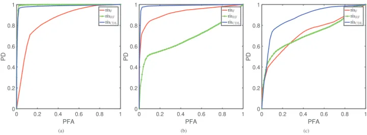
The CD performance of the different methods has been assessed through the empirical receiver operating characteristics (ROC) curves, representing the estimated pixel-wise probability of detection (PD) as a function of the probability of false alarm (PFA). Moreover, two quan-titative criteria derived from these ROC curves have been computed, namely, (i) the area under the curve (AUC), corresponding to the integral of the ROC curve and (ii) the distance between the no detection point (PFA = 1, PD = 0) and the point at the interception of the ROC curve with the diagonal line defined by PFA = 1−PD. For both metrics, the greater the criterion, the better the detection.

5.3. Illustration through real images with real changes

In a first step, experiments are conducted on real images with real changes to emphasize the reliability of the proposed CD method and to illustrate the performance of the proposed algorithmic frame-work. Three distinct scenarios involving 3 pairs of images of different modalities and resolutions, are considered namely,

• Scenario 1 considers two optical images: the acquisition process is very similar for the two images and the image formation processes is characterized by an additive Gaussian noise corruption for both sensors.

• Scenario 2 considers two SAR images: the image formation pro-cess is not the same as for optical images, in particular differing on the noise model, i.e., multiplicative Gamma noise instead of additive Gaussian model.

• _{Scenario 3 considers a SAR image and an optical image: for this} more challenging situation, there is no similarity between the noise corruption models for the two sensors.

To summarize, Scenarios 1 and 2 are dedicated to a pair of images with the same modality, but with a variation on the properties of im-ages between scenarios, e.g., the noise statistics. Note that the proposed CDL algorithm has not been designed to specifically handle these con-ventional scenarios. However, they are still considered to evaluate the performance of the proposed method, in particular w.r.t. the methods specifically designed to address scenario 1 or 2. Conversely, Scenario 3 handles images of different modalities. All considered images have been manually geographically aligned to fulfill the requirements imposed by the considered CD setup.

Table 1

Real images affected by real changes with ground truth for Scenarios 1–3: quantitative detection performance (AUC and distance).

̂ 𝐦F 𝐦̂RF 𝐦̂S 𝐦̂CDL Sc. 1 AUC 0.870426 0.866061 0.750601 0.987379 Dist. 0.831983 0.788579 0.692469 0.950695 Sc. 2 AUC 0.823414 0.93982 0.874743 0.981355 Dist. 0.757076 0.869387 0.80188 0.954995 Sc. 3 AUC_Dist. 0.818246_0.769877 0.862729_0.79658 0.862025 0.966283 0.80078 0.912191

5.3.1. Case of same resolutions and ground truth

For this first set of experiments, images of same spatial resolutions are considered. They are accompanied by a ground truth in the form of an actual change map 𝐦 to be estimated.

Scenario 1: optical vs. optical — The observed images are two

mul-tispectral (MS) optical images with 3 channels representing an urban region in the south of Toulouse, France, before (Fig. 1(a)) and after (Fig. 1(b)) the construction of a road. These 960 × 1560-pixel images are both characterized by a 50cm spatial resolution. The ground-truth change mask 𝐦 is represented inFig. 1(c).Fig. 1depicts the observed images at each date, the ground-truth change mask and the change maps estimated by the four compared methods.

The quantitative results for Scenario 1 are reported inTable 1(lines 1 and 2) and the corresponding ROC curves inFig. 2(a). The analysis of these results shows that the proposed method outperforms state-of-the-art methods for this scenario which involves common changes in urban areas and in MS optical images. Note that, besides the changes, this kind of situation involves a lot of small differences between the two observed images due to the variations in sun the illumination, in the vegetation cover, etc. These effects sometimes are classified as changes, increasing the false alarm rate, especially for state-of-the-art methods. Besides, the proposed method still provides the best detection for this dataset.

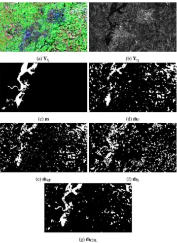
Scenario 2: SAR vs. SAR — For this scenario, two intensity radar

images acquired over the Lake Mulargia region in Sardegna, by the Sentinel-1 satellite in 05/21/2016 (Fig. 3(a)) and 10/30/2016 (Fig. 3(b)) are considered. These 1200 × 1800-pixel images are both characterized by a 10m spatial resolution. This dataset mostly presents seasonal changes, in particular the variation of flooding areas around the Lake Mulargia. The ground-truth change mask is represented in Fig. 3(c). Fig. 3depicts the two observed images, the ground-truth change mask and the change maps estimated by the four compared methods.

The quantitative results for Scenario 2 are reported inTable 1(lines 3 and 4) and the corresponding ROC curves inFig. 2(b). The analysis of these results shows that the proposed method also outperforms the state-of-the-art methods for this scenario. It is a good indication of its flexibility w.r.t. image modalities. Note that, due to the multiplicative noise and the consequent strong fluctuations, the state-of-the-art meth-ods present a lot of false alarms. This effect seems to be attenuated by the proposed method, probably thanks the TV regularization.

Scenario 3: optical vs. SAR — In order to test the performance of the

different compared methods in a multi-modality situation, we consider two images acquired over the Gloucester region, UK, before and after a catastrophic flooding accident in 2007. The before-flooding image, presented inFig. 4(a), is a multispectral optical image with 3 channels acquired by Google Earth while the after-flooding image, depicted in Fig. 4(b), is a radar image acquired by TerraSAR-X. These 2325 × 4133-pixel images are both characterized by a 7.3 m spatial resolution. The ground-truth change mask is represented onFig. 4(c).Fig. 4depicts the observed images at each date, the ground-truth change mask and the change maps estimated by the four comparative methods.

Table 1(lines 5 and 6) reports the quantitative results for Scenario 3 and the corresponding ROC curves are displayed inFig. 2(c). Similarly

Fig. 1. Real images affected by real changes with ground truth, Scenario 1: (a)

observed MS optical image 𝐘𝑡1from the south of Toulouse acquired before the

construc-tion of a new road, (b) observed MS optical image 𝐘𝑡2 acquired after its construction,

(c) ground-truth mask 𝐦 indicating changed areas constructed by photointerpretation, (d) change map ̂𝐦Fof the fuzzy method, (e) change map ̂𝐦RF of the robust fusion

method, (f) change map ̂𝐦Sof the segmentation-based method, and (g) change map

̂

𝐦CDLof proposed method.

as in the previous scenarios, the analysis of these results shows that the proposed method outperforms the state-of-the-art methods even in this more challenging situation involving different image modalities with changes in rural and urban areas. As for Scenario 2, the TV regularization seems to be beneficial to smooth the fluctuations due to the nature of the noise in radar images, which may affect the other compared methods producing more false alarms.

Through this first illustration, we can observe that the segmentation-based method severely underperforms the other methods for scenarios 1 and 2 and underperfoms the proposed method under scenario 1. For brevity, in the following, we will compare only the F and RF methods to the proposed CDL one.

Fig. 2. Real images affected by real changes with ground truth: ROC curves for (a) Scenario 1, (b) Scenario 2, (c) Scenario 3. 5.3.2. Case of different resolutions without ground truth

The previous set of experiments considered pair of images character-ized by the same spatial resolution. As a complementary analysis, this section reports experiments conducted on real images of different spa-tial resolutions with real changes. However, for these 3 pairs of images, corresponding to the three scenarios, no ground truth is available. We first consider a Sentinel-1 SAR image (European Space Agency,2017a) acquired on October 28th 2016. This image is a 540 × 525 interferomet-ric wide swath high resolution ground range detected multi-looked SAR intensity image with a spatial resolution of 10m according to 5 looks in the range direction. Moreover, we also consider two multispectral Landsat 8 (United States Geological Survey, 2017) 180 × 175-pixel images with 30m spatial resolution and composed of the RGB visible bands (Band 2 to 4), acquired over the same region on April 15th 2015 and on September 22th 2015, respectively. Unfortunately, no ground-truth information is available for the chosen dates, as experienced in numerous experimental situations (Bovolo and Bruzzone,2015). How-ever, this region is characterized by interesting natural meteorological changes occurring along the seasons (e.g., drought of the Mud Lake, snow falls and vegetation growth), which helps to visually infer the major changes between observed images and to assess the relevance of the detected changes. All considered images have been manually geographically and geometrically aligned to fulfill the requirements imposed by the considered CD setup. Each scenario is individually studied considering the same denominations as in Section5.3and the same compared methods as in Section5.1.

Scenario 1: optical vs. optical — In this scenario, two different

situations are going to be explored, namely, observed images with the same or different resolutions. The first case considers both Landsat 8 images.Fig. 5depicts the two observed images and the change maps es-timated by the three compared methods. These change maps have been generated according to(12)where the threshold has been adjusted such that each method reveals the most important changes, i.e., the drought of the Mud Lake. As expected, the robust fusion method presents better accuracy in detection since it was specifically designed to handle such a scenario. Nevertheless, the proposed method exhibits very similar results. It is worth noting that some of the observed differences are due to the patch decomposition required by the proposed method. The fuzzy method is able to localize the strongest changes, but low energy changes are not detected. The fuzzy method also suffers from resolution loss due to the size of the patches. Contrary to the proposed method, it does not take the patch overlapping into account, which contributes to decrease the detection accuracy.

Under the same scenario (i.e. optical vs. optical), an additional pair of observed images is used to better understand the algorithm behavior when facing to images of the same modality but with different spatial

resolutions. The observed image pair is composed of the Sentinel-2 image acquired on April 12th 2016 and the Landsat 8 image acquired in September 22th 2015. Note that the two observed images have the same spectral resolution, but different spatial resolutions.Fig. 6depicts the observed images as well as the change maps estimated by the comparative methods. Once again, it is possible to state the similarity of the results provided by the robust fusion method and the proposed one. It also shows the very poor detection performance of the fuzzy method. This may be explained by the difficulty of coupling due to differences in resolutions.

Scenario 2: SAR vs. SAR — In this scenario, observed SAR images

acquired by the same sensor (Sentinel-1) are used to assess the perfor-mance of the fuzzy method and the proposed one. The robust fusion method has not been considered due to the poor results obtained on the synthetic dataset (see Section5.4below).Fig. 7presents the observed images at each date and the change maps recovered by the two compared methods. The same strategy of threshold selection as for Scenario 1 has been adopted to reveal the most important changes. As expected, the proposed method presents a higher accuracy in detection than the fuzzy method. Possible reasons that may explain this difference are (i) the fuzzy method is unable to handle overlapping patches and (ii) the fuzzy method does not exploit appropriate data-fitting terms, in opposite to the proposed one. Besides, as SAR images present strong fluctuations due to their inherent image formation process, the additional TV regularization of the proposed method may contribute to smooth such fluctuations and better couple the dictionaries.

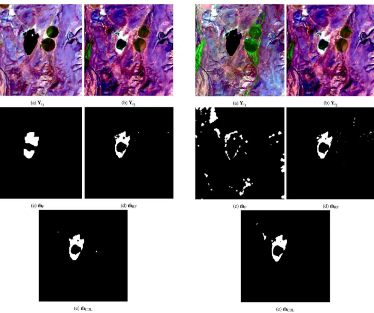
Scenario 3: optical vs. SAR — For this scenario, once again, two

different situations are addressed: images with the same or different spatial resolutions. The first one considers the Sentinel-2 MS image acquired on April 12th 2016 and the Sentinel-1 SAR image acquired in October 28th 2016.Fig. 8presents the observed images and the change maps derived from the fuzzy and proposed methods. To derive the change maps, the thresholding strategy is the same as for all previous scenarios. Once again, the proposed method shows better detection accuracy performance than the fuzzy one. It is important to emphasize the similarity of the results achieved in Scenario 3 and Scenario 2 for images acquired at the same date. Note also that this similarity can be observed for the proposed method, which contributes to increase its reliability for CD between multimodal images.

The second observed image pair consists in a Sentinel-1 SAR image acquired on April 12th 2016 and a Landsat 8 MS image acquired on September 22th 2015. This pair represents the most challenging situa-tion among all presented images, namely differences in both modalities and resolutions.Fig. 9presents the observed images at each date and the recovered change maps. For this last experiment, the proposed method presents better accuracy in detection than the fuzzy one. All

Fig. 3. Real images affected by real changes with ground truth, Scenario 2: (a)

observed radar image 𝐘𝑡1 from the Lake Mulargia acquired in 05/21/2016 by Sentinel

1, (b) observed radar image 𝐘𝑡2 from the Lake Mulargia acquired in 10/30/2016

by Sentinel 1, (c) ground-truth mask 𝐦 indicating changed areas constructed by photointerpretation, (d) change map ̂𝐦F of the fuzzy method, (e) change map ̂𝐦RF

of the robust fusion method, (f) change map ̂𝐦S of the segmentation-based method,

and (g) change map ̂𝐦CDLof proposed method.

Fig. 4. Real images affected by real changes with ground truth, Scenario 3: (a)

observed MS optical image 𝐘𝑡1from Gloucester region acquired before the flooding by

Google Earth, (b) observed radar image 𝐘𝑡2 from Gloucester region acquired after the

flooding by TerraSAR-X, (c) ground-truth mask 𝐦 indicating changed areas constructed by photointerpretation, (d) change map ̂𝐦Fof the fuzzy method, (e) change map ̂𝐦RF

of the robust fusion method, (f) change map ̂𝐦Sof the segmentation-based method,

and (g) change map ̂𝐦CDLof proposed method.

differences in all previous situations can be observed in this scenario, culminating in the poor detection performance of the fuzzy method and a reliable change map for the proposed one.

5.4. Statistical performance assessment

Finally, the last set of experiments aims at statistically evaluating the performance of compared algorithms thanks to simulations on real images affected by synthetic changes. More precisely, in the case of multi-band images, a dedicated CD evaluation protocol was proposed by Ferraris et al.(2017a) based on a single high spatial resolution hyperspectral reference image. The experiments conducted in this work follow the same strategy. Two multimodal reference images acquired at the same date have been selected as change-free latent images. By conducting simple copy–paste of regions, as inFerraris et al.(2017a), changes have been generated in both images as well as their corre-sponding ground-truth maps. This process allows synthetic yet realistic changes to be incorporated within one of these latent images, w.r.t. a pre-defined binary reference change mask locating the pixels affected by these changes and further used to assess the performance of the CD algorithms. This process is detailed in what follows.

5.4.1. Simulation protocol

Reference images — The reference images 𝐗ref 1 and 𝐗

ref 2 used in this experiment comes from two largely studied open access satel-lite sensors, namely Sentinel-1 (European Space Agency, 2017a) and