Contributions to the modelling of acoustic and elastic wave propagation in large-scale domains with boundary element methods
109
0
0
Texte intégral
Figure
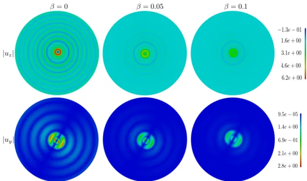
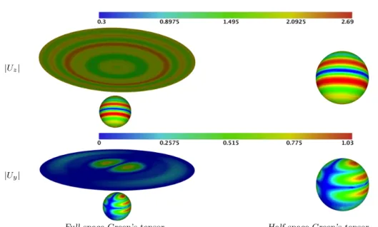
![Figure 1.3: Diffraction of an oblique incident plane P-wave by a semi-ellipsoidal canyon: hor- hor-izontal (left) and vertical (right) computed displacement on canyon surface and meshed part of free surface (normalized frequency κ s a/π = 2); from [14]](https://thumb-eu.123doks.com/thumbv2/123doknet/14704114.747573/18.893.149.826.672.903/diffraction-incident-ellipsoidal-vertical-computed-displacement-normalized-frequency.webp)
+7
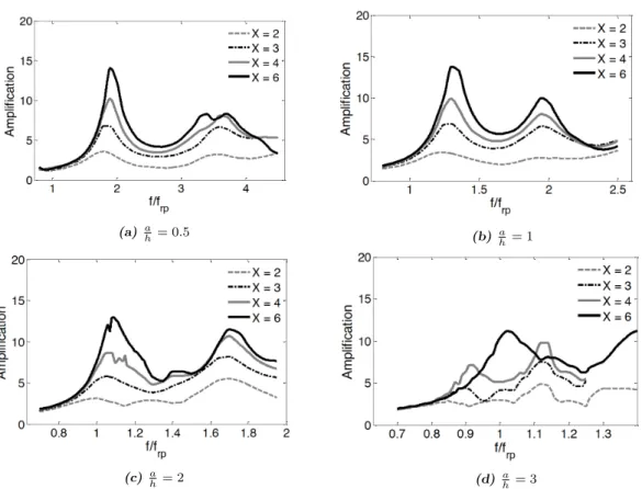
![Figure 1.9: Amplification at the top of the 3D basin (with 5% damping) due to vertically incident S-waves with different equivalent shape ratios (from [4]).](https://thumb-eu.123doks.com/thumbv2/123doknet/14704114.747573/23.893.101.753.145.410/figure-amplification-damping-vertically-incident-different-equivalent-ratios.webp)
![Figure 1.12: Circular surface footing on a hemispherical basin. Computation of the normalised impedance (K 11 ): comparison of the FM-BEM (COFFEE), FEM-BEM coupling (Code Aster) solutions and the reference solution from [Sieffert 1992] (Sieffert homogeneou](https://thumb-eu.123doks.com/thumbv2/123doknet/14704114.747573/27.893.115.738.283.518/circular-hemispherical-computation-normalised-impedance-comparison-solutions-homogeneou.webp)
Documents relatifs