HAL Id: tel-03116812
https://tel.archives-ouvertes.fr/tel-03116812
Submitted on 20 Jan 2021HAL is a multi-disciplinary open access archive for the deposit and dissemination of sci-entific research documents, whether they are pub-lished or not. The documents may come from teaching and research institutions in France or abroad, or from public or private research centers.
L’archive ouverte pluridisciplinaire HAL, est destinée au dépôt et à la diffusion de documents scientifiques de niveau recherche, publiés ou non, émanant des établissements d’enseignement et de recherche français ou étrangers, des laboratoires publics ou privés.
kernels for machine learning
Filip Igor Pawlowski
To cite this version:
Filip Igor Pawlowski. High-performance dense tensor and sparse matrix kernels for machine learning. Distributed, Parallel, and Cluster Computing [cs.DC]. Université de Lyon, 2020. English. �NNT : 2020LYSEN081�. �tel-03116812�
THÈSE de DOCTORAT DE L’UNIVERSITÉ DE LYON
opérée parl’École Normale Supérieure de Lyon
École Doctorale N◦512
École Doctorale en Informatique et Mathématiques de Lyon
Spécialité : Informatique
présentée et soutenue publiquement le 11/12/2020, par :
Filip Igor PAWLOWSKI
High-performance dense tensor and sparse matrix
kernels for machine learning
Noyaux de calcul haute-performance de tenseurs denses et
matrices creuses pour l’apprentissage automatique
Devant le jury composé de :
Alfredo BUTTARI Chercheur, CNRS Rapporteur
X. Sherry LI Directrice de recherche,
Lawrence Berkeley National Lab., Etats-Unis,
Rapporteure
Ümit V. ÇATALYÜREK Professeur, Georgia Institute of Tech., Etats-Unis,
Examinateur Laura GRIGORI Directrice de recherche, Inria Examinatrice
Bora UÇAR Chercheur, CNRS Directeur de thèse
Albert-Jan N. YZELMAN Chercheur, Huawei Zürich Re-search Center, Suisse
Résumé français . . . vi
1 Introduction 2 1.1 General background. . . 2
1.1.1 The cache memory and blocking . . . 3
1.1.2 Machine and cost model . . . 4
1.1.3 Parallel algorithm analysis . . . 6
1.1.4 Memory allocation and partitioning . . . 7
1.2 Thesis outline . . . 7 1.2.1 Tensor products . . . 8 1.2.2 Sparse inference . . . 9 2 Tensor computations 12 2.1 Introduction . . . 13 2.2 Related work . . . 14
2.3 Sequential tensor–vector multiplication . . . 17
2.3.1 Tensor layouts. . . 17
2.3.2 Two state-of-the-art tensor–vector multiplication algorithms . . . 19
2.3.3 Block tensor–vector multiplication algorithms . . . 20
2.3.4 Experiments . . . 22
2.4 Shared-memory parallel tensor–vector multiplication. . . 35
2.4.1 The loopedBLAS baseline . . . 37
2.4.2 Optimality of one-dimensional tensor partitioning . . . 38
2.4.3 Proposed 1D TVM algorithms. . . 40
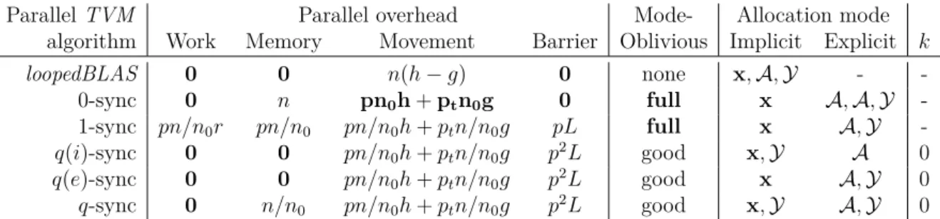
2.4.4 Analysis of the algorithms . . . 42
2.4.5 Experiments . . . 46
2.5 Concluding remarks . . . 50
3 Sparse inference 53 3.1 Introduction . . . 54
3.1.1 Sparse inference . . . 54
3.1.2 Sparse matrix–sparse matrix multiplication. . . 55
3.1.3 Hypergraph partitioning . . . 56
3.1.4 Graph Challenge dataset . . . 57
3.1.5 State of the art . . . 58 ii
3.2 Sequential sparse inference . . . 60
3.2.1 SpGEMM-inference kernel . . . 60
3.2.2 Sparse inference analysis . . . 62
3.2.3 SpGEMM-inference kernel for partitioned matrices . . . 63
3.3 Data-, model- and hybrid-parallel inference . . . 64
3.3.1 Data-parallel inference . . . 64
3.3.2 Model-parallel inference . . . 67
3.3.3 Hybrid-parallel inference and deep inference . . . 72
3.3.4 Implementation details . . . 74
3.4 Experiments . . . 74
3.4.1 Setup . . . 75
3.4.2 The tiling model-parallel inference results . . . 76
3.4.3 The tiling hybrid-parallel inference results . . . 80
3.5 Concluding remarks . . . 82 4 Conclusions 83 4.1 Summary . . . 83 4.1.1 Summary of Chapter 2 . . . 83 4.1.2 Summary of Chapter 3 . . . 84 4.2 Future work . . . 86 4.2.1 Tensor computations . . . 86 4.2.2 Sparse networks . . . 87 Bibliography 93
2.1 The looped tensor–vector multiplication . . . 20
2.2 The unfold tensor–vector multiplication. . . 21
2.3 The block tensor–vector multiplication algorithm . . . 22
2.4 The next block according to a ρπ layout. . . 23
2.5 The next block according to a Morton layout. . . 24
2.6 A basic higher-order power method . . . 35
2.7 The q-sync parallel TVM algorithm. . . . 41
2.8 The interleaved q(i)-sync parallel TVM algorithm.. . . 42
2.9 The explicit q(e)-sync parallel TVM algorithm. . . . 42
3.1 The SpGEMM-inference kernel. . . 61
3.2 The SpGEMM-inference kernel for partitioned matrices.. . . 65
3.3 The model-parallel inference at layer k. . . . 69
3.4 The tiling model-parallel inference. . . 73
3.5 The latency-hiding model-parallel layer-k inference. . . . 75
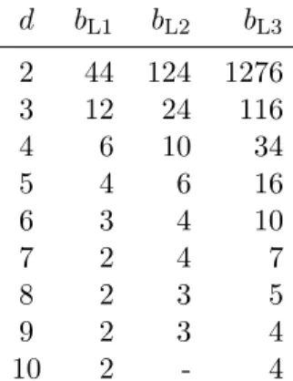
2.1 Plot of the effective bandwidth (in GB/s) of the copy kernels. . . 26
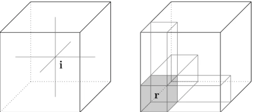
2.2 Illustration of elements lying on all axes going through tensor element(s). 39
3.1 The staircase matrix of a neural network. . . 71
3.2 Plot of the run time of the data-parallel and the tiling model-parallel in-ference using 5 layers on Ivy Bridge. . . 77
3.3 Plot of the run time of the data-parallel and the tiling model-parallel in-ference using 5 layers on Cascade Lake. . . 78
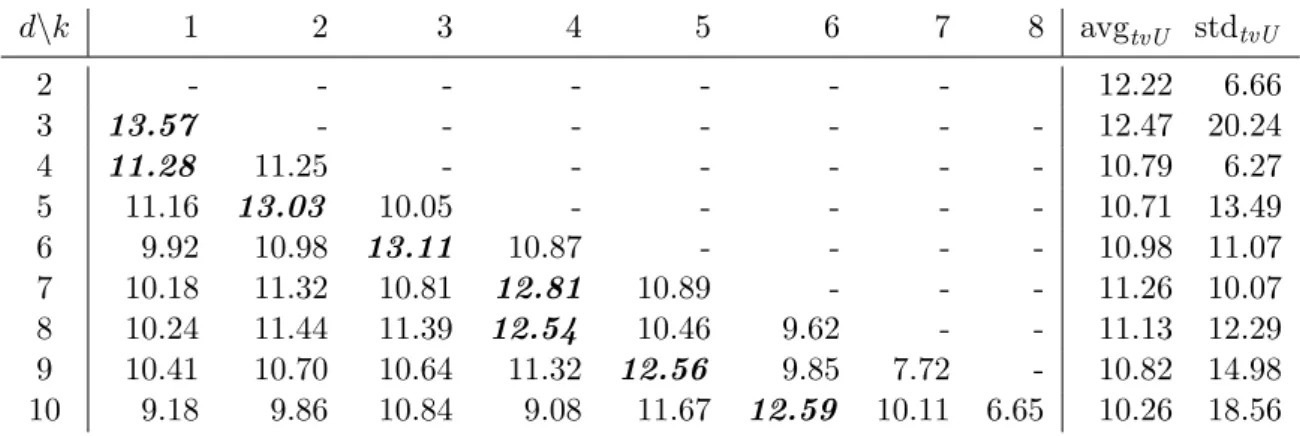
Dans cette thèse, nous développons des algorithmes à haute performance pour certains calculs impliquant des tenseurs denses et des matrices creuses. Nous abordons les noy-aux de calculs qui sont utiles pour les tâches d’apprentissage automatique, telles que l’inférence avec les réseaux neuronaux profonds (DNN). Nous développons des structures de données et des techniques pour réduire l’utilisation de la mémoire, pour améliorer la localisation des données et donc pour améliorer la réutilisation du cache des opérations du noyau. Nous concevons des algorithmes séquentiels et parallèles à mémoire partagée. Dans la première partie de la thèse, nous nous concentrons sur les noyaux de calculs de tenseurs denses. Les noyaux de calculs de tenseurs comprennent la multiplication vecteur (TVM), la multiplication matrice et la multiplication tenseur-tenseur. Parmi ceux-ci, la TVM est la plus limitée par la bande passante et constitue un élément de base pour de nombreux algorithmes. Nous nous concentrons sur cette opéra-tion et développons une structure de données et des algorithmes séquentiels et parallèles pour celle-ci. Nous proposons une nouvelle structure de données qui stocke le tenseur sous forme de blocs, qui sont ordonnés en utilisant la courbe de remplissage de l’espace connue sous le nom de courbe de Morton (ou courbe en Z). L’idée principale consiste à diviser le tenseur en blocs suffisamment petits pour tenir dans le cache et à les stocker selon l’ordre de Morton, tout en conservant un ordre simple et multidimensionnel sur les éléments individuels qui les composent. Ainsi, des routines BLAS haute performance peu-vent être utilisées comme micro-noyaux pour chaque bloc. Nous évaluons nos techniques sur un ensemble d’expériences. Les résultats démontrent non seulement que l’approche proposée est plus performante que les variantes de pointe jusqu’à 18%, mais aussi que l’approche proposée induit 71% de moins d’écart-type d’échantillon pour le TVM dans les différents modes possibles. Enfin, nous montrons que notre structure de données s’étend naturellement à d’autres noyaux de calculs de tenseurs en démontrant qu’elle offre des performances jusqu’à 38% supérieures pour la méthode de puissance d’ordre supérieur. Enfin, nous étudions des algorithmes parallèles en mémoire partagée pour la TVM qui utilisent la structure de données proposée. Plusieurs algorithmes parallèles alternatifs ont été caractérisés théoriquement et mis en œuvre en utilisant OpenMP pour les com-parer expérimentalement. Nos résultats sur un maximum de 8 processeurs montrent une performance presque maximale pour l’algorithme proposé pour les tenseurs à 2, 3, 4 et 5 dimensions.
Dans la deuxième partie de la thèse, nous explorons les calculs creux dans les réseaux de neurones en nous concentrant sur le problème d’inférence profonde creuse à haute
performance. L’inférence creuse de DNN représente la tâche où les DNN creux clas-sifient un lot d’éléments de données formant, dans notre cas, une matrice creuse. La performance de l’inférence creuse dépend de la parallélisation efficace de la multiplication matrice creuse-matrice creuse (SpGEMM) répétée pour chaque couche de la d’inférence. Nous caractérisons d’abord les algorithmes SpGEMM séquentiels efficaces pour notre cas d’utilisation. Nous introduisons ensuite l’inférence modèle-parallèle, qui utilise un titionnement bidimensionnel des matrices de poids obtenues à l’aide du logiciel de par-titionnement des hypergraphes. La variante modèle-parallèle utilise des barrières pour synchroniser entre les couches. Enfin, nous introduisons les algorithmes de tuilage modèle-parallèle et de tuilage hybride, qui augmentent la réutilisation du cache entre les couches, et utilisent un module de synchronisation faible pour cacher le déséquilibre de charge et les coûts de synchronisation. Nous évaluons nos techniques sur les données du grand réseau de l’IEEE HPEC 2019 Graph Challenge sur les systèmes à mémoire partagée et nous rapportons jusqu’à 2 fois de l’accélération par rapport à la référence.
Introduction
This thesis is in the field of performance computing and focuses on finding high-performance algorithms which solve computational problems involving dense tensors and sparse matrices. Traditional computational problems involve dense matrix and sparse matrix computations with potentially only a few matrices, as in the preconditioned it-erative methods or multigrid methods for solving linear systems. Up-and-coming tasks in data analysis and machine learning deal with multi-modal data and involve a large number of matrices. We see two classes of computational problems associated with these tasks: those having dense tensors, which are collections of dense matrices, and those having a large number of sparse matrices. We identify frequently used kernels in these problems. We discuss a machine model and a cost model to quantify the data movement of parallel algorithms. We develop data structures and sequential kernel implementa-tions which increase cache reuse. We then develop shared-memory parallel algorithms and analyze their practical effects using the proposed cost model as well as the effects of the proposed data structures on high-end computer systems. We use those kernels in applications concerning tensor decomposition and analysis, and in inference with sparse neural networks.
In this chapter, we first give a general background that underlines our approach to the two subjects of the thesis in Section 1.1. Section 1.2 then gives an outline of the thesis by summarizing the problems, contributions, and the main results.
1.1
General background
In this thesis, we are interested in designing algorithms and techniques that apply to modern architectures. As the memory throughput grows much slower than the ma-chine’s computational power, increasingly many workloads are bottlenecked by memory, on modern machines. On modern hardware, a computing unit has multiple local mem-ory storages connected to it. One such memmem-ory, caches, have lower latency and higher bandwidth but smaller size when compared to main memory. The cache memory is a hardware optimization design to store the data a computing unit requires as it might be used again in nearby future. On parallel machines, when these computing units are
connected and share their local memories with the other computing units, a common characteristic is that the time to access local memory is much shorter than to access the local memories of other units. This gives rise to the notion of local and remote mem-ories for each unit. Shared-memory architectures with this characteristic are known as the Non-Uniform Memory Access (NUMA) machines, as the main memory accesses have different latency and throughput. To design efficient parallel algorithms we must be able to estimate their costs on such hardware.
This section is organized as follows. In Section 1.1.1 we describe the cache memory and the programming techniques that we adopt in this thesis to use the cache memory effectively. In Section 1.1.2, we describe a bridging model of NUMA hardware which includes a model of parallel computation and a cost model we use to analyze paral-lel algorithms. In Section 1.1.3, we introduce the concept of parallel overheads we use to compare parallel algorithms with respect to the best sequential alternative. In Sec-tion 1.1.4we discuss allocation techniques which allow to effectively distribute data on a shared-memory machine.
1.1.1
The cache memory and blocking
The cache memory is an on-chip memory which is closer to the CPU and hence faster to access, but also very small due to its high production costs. Typically, CPUs contain multiple levels of caches where the higher level caches have higher latencies and lower bandwidths, but greater size. This is done as programs have tendency to reuse the same data in a short period of time, which is referred to as temporal locality. The computing unit first looks up data in each level of cache. If the cache contains the required element, it is called a cache hit. Otherwise, if the element has not been found, it is fetched from the main memory and loaded into cache and processor registers; this is called a cache miss. The hardware policy governs which elements to then evict from cache when it reaches its capacity. A perfect architecture usually assumes the Least Recently Used (LRU) policy, which evicts the least recently used elements first.
In the thesis, we use a well-known software optimization technique to increase the temporal locality of algorithms known as the loop blocking, or loop tiling. This technique reorganizes the computation in the program to repeatedly operate on small parts of data, known as blocks or tiles. The size of a block should be such that a block’s data fits in cache. If the block’s data fits in cache, then the number of cache misses reduces and hence one sees improved performance. We note that such a blocking is justified only under two conditions. First, a program must reuse the data in blocks as opposed to
streaming them, that is, touching the data only once. Second, the original data should
be much larger than the cache size; otherwise, blocking becomes an overhead. Optimal block sizes could be determined statically on a per-machine basis, either analytically or via (manual or automated) experimentation. The latter approach results in a process known as parameter tuning.
Spatial locality is another property of programs which is crucial to performance. It
occurs when a program accesses a data item and subsequently requires another data item lying in close-by memory areas; a special case is when a program iterates over successive
memory addresses in a streaming fashion. We note that blocking does not necessarily achieve spatial locality, which itself relates not only to the computation but also to the data layout. In the thesis, we modify the storage of input data and propose new data layouts which improve spatial locality of blocking algorithms.
1.1.2
Machine and cost model
At an abstract level, a shared-memory parallel NUMA machine consists of ps connected
processors, or sockets. Each socket consists of ptthreads thus yielding a total of p = pspt
threads. Each socket has local memory connected to it: the cache, RAMs, and the main memory. The sockets are connected with each other via a communication bus such that the memory is shared and forms a global address space. A thread executing on a socket may access the local memory of the socket faster than the remote memory of the other sockets; a NUMA effect.
We use a set of parameters to characterize such a shared-memory NUMA machine: • r, the time a flop operation takes in seconds;
• L, the time in which a barrier completes in seconds;
• g, the time required to move a byte from local memory to a thread in seconds; and • h, the time to move a byte from remote memory to the thread in seconds.
Thus, g is inversely proportional to the intra-socket throughput while h is inversely pro-portional to the inter-socket memory throughput per socket. These parameters together with ps and pt fully characterize a machine and allow quantifying the behavior of a
pro-gram running on that machine.
The following model allows quantifying the cost of a parallel program. Any parallel program may be viewed as a series of S barriers with S + 1 phases in between them. Therefore, each thread q ∈ {0, . . . , p − 1} executes S + 1 different phases, which are numbered using integer s, 0 ≤ s ≤ S. We quantify the computation in terms of the number of floating point operations, or flops, which includes all scalar operations. We use Wq,sto count the local computation at thread q in flops at phase s. For each thread,
we distinguish between the socket and inter-socket data movement. While the intra-socket data movement Uq,scounts the data thread q reads and writes in the local memory
in words at phase s, the inter-socket data movement Vq,s counts the data items in words
q reads and writes in the remote memory in words at phase s. We use Mq,s to denote
the storage requirement by thread q at phase s in bytes. While these fully quantify an algorithm, their values depend on the number of threads p as well as on any problem parameters.
In general, the cost of each phase s is proportional to the slowest thread, which completes in maxq{Wq,sr+Uq,sg+Vq,sh}. Thus, the time in which an algorithm consisting
of S + 1 phases completes is T(n, p) = S X s=0 " max q∈{0,...,p−1}{Wq,sr+ Uq,sg+ Vq,sh} # + SL seconds. (1.1)
However, if the local computational may be overlapped with data movement, the same algorithm completes in T(n, p) = S X s=0 " max{ max q∈{0,...,p−1}Wq,sr,q∈{0,...,p−1}max {Uq,sg+ Vq,sh} # }+ SL seconds. (1.2) Note that for any s:
max
q∈{0,...,p−1}{Wq,sr+ Uq,sg+ Vq,sh}/max{ maxq∈{0,...,p−1}Wq,sr,q∈{0,...,p−1}max {Uq,sg+ Vq,sh}} ≤2,
and that this upper bound is reached only if max
q∈{0,...,p−1}Wq,sr =q∈{0,...,p−1}max {Uq,sg+ Vq,sh}.
Minimizing each of the total asymptotic costs of computation, data movement and syn-chronization for any input and number of threads, i.e., minimizing
Twork = S X s=0 max q∈{0,...,p−1}Wq,sr Tdata = S X s=0 max q∈{0,...,p−1}{Uq,sg+ Vq,sh} Tsync= SL, (1.3)
thus minimizes both the overlapping and non-overlapping versions of T (n, p). The final cost metric we use is the storage requirement of a parallel algorithm. It is the maxi-mum storage requirement M(n, p) = maxq∈{0,...,p−1}PSs=0Mq,s(n, p) per thread during all
phases.
We note that in practice, many problems do not have an algorithmic solution which minimizes all three costs simultaneously. In the thesis, we propose algorithms which have various ratios between these costs. The final implementation may be chosen based on the number of threads, the problem size, and the parameters values r, g, h and L of the machine.
Related models. The Random Access Machine (RAM) is an agreed upon model of
computation for sequential machines, while for parallel computing the Bulk Synchronous Parallel (BSP) and Communicating Sequential Processes (CSP) models quantify the costs of parallel programs effectively under different scenarios. While our model focuses on data movement, the BSP [61] is another bridging model of hardware which explicitly models communication. The originally proposed BSP model is also known as the flat BSP model, as it states that all processes take equal time to communicate with each other and does not capture the NUMA effects. Variants of the BSP model which capture NUMA effects and provide a cost model are the BSPRAM [57] and the multi-BSP [62]. The multi-BSP model also considers multiple levels of memory locality, e.g., a shared-memory and distributed-shared-memory parallel machine where shared-memory may be seen at three
levels. Another parallel model of computation is the Parallel Random Access Machine (PRAM) [22] which assumes that the synchronization issues are resolved by the hardware itself and that communication has a constant cost. Therefore, it cannot serve as a tool to model data movement costs.
1.1.3
Parallel algorithm analysis
A basic metric to measure performance of a parallel algorithm is the ratio of a sequential algorithm run time Tseq to the parallel run time for p threads,
S(n, p) = Tseq(n) T(n, p).
Ideally, the speedup of a parallel program grows linearly with p for a constant problem size n. However, Amdahl’s law states that this is not attainable in practice as most parallel algorithms possess a parallel overhead
O(n, p) = pT (n, p) − Tseq(n).
It may be thought of as the execution time of the part of the program which cannot be parallelized, i.e., its critical section. Except for trivially parallel algorithms, the critical section increases with n and p. Another metric to evaluate performance of a parallel algorithm is the parallel efficiency defined as the ratio between speedup and the number of threads:
E(n, p) = S(n, p)
p =
Tseq(n)
pT(n, p).
Gustafson’s law states that the speedup of a parallel program grows linearly with p, that is, its efficiency remains constant, if n increases. This is true for most parallel algorithms as Tseq grows with n as well, thus amortizing the impact of the overhead on efficiency:
E(n, p) = 1 − O(n, p) O(n, p) + Tseq(n)
.
The above formula allows to compute how fast n should grow to retain the same parallel efficiency as p increases and vice versa, giving rise to the concept of iso-efficiency. Strongly
scalingalgorithms have that the overhead O(n, p) is independent of p, which is unrealistic,
while weakly scaling algorithms have that the ratio O(pn, p)/Tseq(pn) is constant;
iso-efficiency instead tells us a much wider range of conditions under which the algorithm scales. We note that the total number of threads an algorithm employs need not be equal to the number of cores a given machine holds; it can be less when considering strong scalability, and it can be more when exploring the use of hyperthreads.
Using the parallel costs defined in (1.3), we subdivide the parallel overhead and define the following parallel overheads for each of the corresponding parallel costs to quantify parallel algorithms:
Owork(n, p) = pTwork(n, p) − Tseq-work(n)
Odata(n, p) = pTdata(n, p) − Tseq-data(n)
We note that when counting the data movement overhead Odata(n, p) for algorithms
which use blocking, we assume a perfect caching occurs for blocks and that they do not contribute to the overhead. All overheads should compare against the best performing sequential algorithm, which may be drastically different than the parallel algorithm for
p= 1. Finally, we define the parallel storage overhead Omem(n, p) = pM(n, p) − Mseq(n),
where Mseq is the storage size required by the best sequential algorithm.
The final metric we use is the arithmetic intensity, which is a ratio between the number of floating point operations an algorithm performs versus the memory size it touches during the computation. We determine the arithmetic intensity of the best sequential algorithm to determine how likely the algorithm is to fully utilize the memory bandwidth of a machine rather than its computational power. While the bottleneck of compute-bound algorithms is the computational power of a machine, the bottleneck of bandwidth-bound algorithms is the memory speed. However, this does not preclude memory optimizations from benefiting compute-bound kernels, but rather states that these will improve the run time to a smaller degree.
1.1.4
Memory allocation and partitioning
On shared-memory systems, each processor has local memory to which it accesses faster than remote memory areas. We assume that threads taking part in a parallel computation are pinned to a specific core, meaning that threads will not move from one core at run time. A pinned thread has a notion of local memory: namely, all addresses that are mapped to the memory controlled by the processor the thread is pinned to. This gives rise to two distinct modes of use for shared memory areas: the explicit versus interleaved modes. If a thread allocates, initializes, and remains the only thread using this memory area, we dub its use explicit. In contrast, if the memory pages associated with an area cycle through all available memories, then the use is called interleaved. The latter mode is enabled by NUMA-ctl library [47]. If a memory area is accessed by all threads in a uniformly random fashion, then it is advisable to interleave it to achieve high throughput.
1.2
Thesis outline
The main contributions of the thesis are discussed in two chapters. Chapter 2 focuses on problems in dense tensor computations, while Chapter 3treats the problem of sparse inference. In both chapters, the main elements of our approach are as follows. We propose algorithms and implement them on shared-memory systems. We analyze the proposed algorithms theoretically using the metrics discussed in Section1.1.3. We also analyze the proposed algorithms experimentally, where parallel codes use OpenMP and are run on shared memory systems.
1.2.1
Tensor products
In Chapter2, we investigate computations on dense tensors (or multidimensional arrays) in d modes (dimensions). Much like matrices can be multiplied with vectors or matri-ces, tensors can be multiplied with vectors, matrimatri-ces, or tensors. These multiplication operations are called tensor–vector multiplication (TVM), tensor–matrix multiplication (TMM), and tensor–tensor multiplication (TTM). These multiplication operations apply to specific modes; each multiplication can operate on a subset of modes of the input ten-sor. We dub algorithms such as the TVM, TMM, and TTM kernels. Much in line with the original Basic Linear Algebra Subprograms (BLAS) definition [19,20], we classify the TVM as a generalized BLAS level-2 (BLAS2) kernel, while we classify the TMM,
TTM, and Khatri-Rao products [27] as generalized BLAS3 ones. These kernels form
the core components in tensor computation algorithms [4]; one example is the computa-tion of Candecomp/Parafac decomposicomputa-tion of tensors using the alternating least squares method [5] and its computationally efficient implementations [27,31,52].
In Chapter2, we first focus on sequential algorithms to optimize the TVM operations. We define a tensor kernel to be mode-aware if its performance strongly depends on the mode in which the kernel is applied; otherwise, we define the kernel to be mode-oblivious. This informal definition is in-line with the more widely known concept of cache-aware versus cache-oblivious algorithms [23]. We propose block-wise storage for tensors to mode-obliviously support common tensor kernels. We closely investigate the TVM kernel, which is the most bandwidth-bound due to low arithmetic intensity (defined in Section 1.1.3). Thus, among the three multiplication operations, TVM is the most difficult one to achieve high performance. However, as guaranteeing efficiency for bandwidth-bound kernels is harder, the methods used for them can be extended to others. Efficient TMM and
TTM kernels, in contrast, often make use of the compute-bound general matrix–matrix
multiplication (BLAS3).
Tensors are commonly stored in an unfolded fashion, which corresponds to a higher-dimensional equivalent of row-major or column-major storage for matrices. While a matrix can be unfolded in two different ways, a d-dimensional tensor can be stored in
d! different ways, depending on the definition of precedence of the modes. We discuss
previous work in tensor computations, including tensor storage and develop a notation for precisely describing a tensor layout in computer memory and for describing how an algorithm operates on tensor data stored that way.
We discuss various ways for implementing the TVM. The first one notes TVM’s similarity to the matrix–vector multiplication (MVM). It takes a tensor, the index of a mode, and a vector of size conformal to that mode’s size and performs scalar multiply and add operations. In fact the MVM kernel can be used to carry out a TVM by either (i) reorganizing the tensor in memory (unfolding the tensor) followed by a single MVM; or (ii) reinterpreting the tensor as a series of matrices, on which a series of MVM operations are executed. We describe how to implement them using BLAS2, resulting in two highly optimized baseline methods. We then introduce our proposed blocked data structure for efficient, mode-oblivious performance. A blocked tensor is a tensor with smaller equally-sized tensors as its elements. We consider only the case where smaller tensor blocks are
stored in an unfolded fashion and are processed using one or more BLAS2 calls. We define two block layouts, which determine the order of processing of the smaller blocks: either a simple, natural ordering of dimensions or one inferred from the Morton order [45].
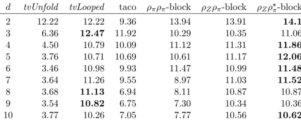
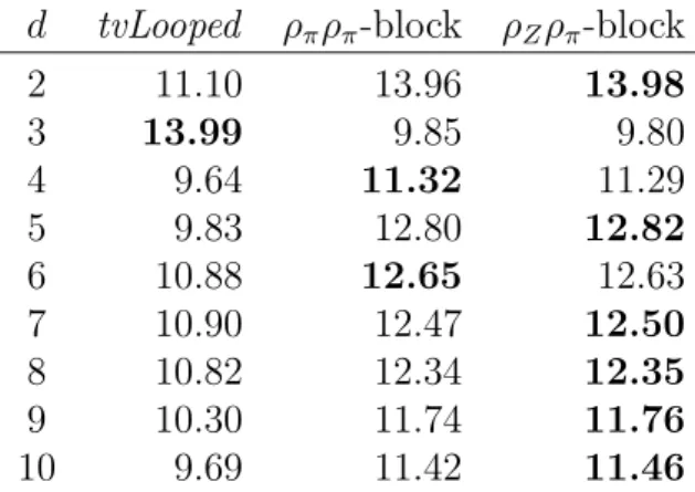
The experiments show that the Morton order blocked data structure offers higher performance on the TVM kernel when compared to the state-of-the-art methods. It also maintains a significantly lower standard deviation of performance when the TVM is applied on different modes, thus indeed achieving mode-oblivious behavior. We use the proposed data structure and TVM algorithm to implement a method used in tensor decomposition and analysis, and show that the superior performance observed for the
TVM is retained.
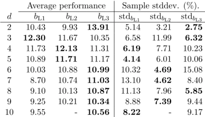
We then turn our attention to shared-memory parallel TVM algorithms based on the proposed sequential algorithm and Morton-blocked layout. We prove that a one-dimensional partitioning is communication optimal under an assumption that the TVM kernel is applied in a series, each time to the input tensor. We characterize several alternative parallel algorithms which follow the algorithmic bound in (1.1) and implement two variants using OpenMP which we compare experimentally. Our results on up to 8 socket systems show near peak performance for the proposed algorithm for 2, 3, 4, and 5-dimensional tensors.
The work we present in this chapter has been published in a journal [50] and a conference [49]:
• F. Pawłowski, B. Uçar, and A. N. Yzelman, A multi-dimensional Morton-ordered block storage for mode-oblivious tensor computations, Journal of Computational Science, 33 (2019), pp. 34–44. This paper discusses the mode-oblivious storage and the sequential kernel.
• F. Pawłowski, B. Uçar, and A. N. Yzelman. High performance tensor–vector mul-tiplication on shared-memory systems. In R. Wyrzykowski, E. Deelman, J. Don-garra, and K. Karczewski, editors, Parallel Processing and Applied Mathematics, pages 38–48, Cham, 2020. Springer International Publishing. This paper discusses the parallel tensor–vector multiplication algorithm design.
1.2.2
Sparse inference
In Chapter 3, we explore the sparse computations in neural networks by focusing on the high-performance deep inference problem with sparsely connected neural networks. Sparse inference is the task of classifying a number of data items using a sparse neural network. This problem was posed by the IEEE HPEC Graph Challenge 2019 [33]. In the case of the Graph Challenge, the data items are also sparse, thus forming a sparse input as well.
In summary, a neural network (NN) consists of d ∈ N layers of neurons, where the neurons at each level combine outputs of all neurons from the previous layer by a weighted sum, potentially add biases, and apply an activation function to produce an output for the next layer. The first layer is called the input layer and the last layer is called the output layer. If a neuron does not combine the output of all neurons in the previous
layer, then the neural network becomes sparse. In the sparse inference, the aim is to classify a given input into one of the classes decided so far. The typical example [36] is to classify or map a given hand-written digit into the intended digit 0, . . . , 9.
The weighted combination at layer k of the outputs of the neurons from the previous layer can be accomplished by a matrix–matrix multiply of the form X(k)W(k), where W(k)
lists the weights and X(k) is the output of the previous layer. With the biases and the
activation function, the whole inference then can be described as computing the final
classification matrix X(d) ∈Rn×c from the input feature matrix X(0):
X(d) = f(· · · f(f(X(0)W(0)+ enb(0) T )W(1) + enb(1) T ) · · · W(d−1)+ e nb(d−1) T ) .
Here, X(0) consists of sparse feature vectors, one row for each data instance to be
classified, and X(d) has a row for each data instance and a column for each
poten-tial output class. The function f : R → R is the activation function to be applied element-wise, b(k) ∈ Rnk+1×1 is a vector of bias at layer k, and e
n is the vector of ones,
en = (1, 1, . . . , 1)T ∈Rn×1. In our case, the input data instances are sparse, the
connec-tions are sparse and hence the weight matrices are sparse, all together these give rise to the sparse inference problem of Chapter 3. There are different activation functions; our application in Chapter 3 uses one called ReLU, which replaces negative entries by zeros. The performance of sparse inference hinges on the performance of sparse matrix–sparse matrix multiplication (SpGEMM) as can be seen in the equation above. We first observe that the computation of SpGEMM may be combined with the activation function and the bias addition at each layer. We propose a modified SpGEMM kernel which iteratively computes sparse inference by computing all operations and a variant of this kernel to be used within one of the parallel inference variants in which the input and output matrices are partitioned.
After analyzing the state-of-the-art inference algorithm, the data-parallel inference, we propose a model-parallel one. These algorithms differ in the way the feature and the weight matrices are partitioned. Partitioning the feature matrix row-wise yields the data-parallel inference, in which each thread executes a series of SpGEMMs interleaved with the activation function without synchronizations, in an embarrassingly parallel fash-ion. Partitioning the neural network yields the model-parallel inference, which induces a partitioning on the feature matrix and requires barriers to synchronize at layers.
Typically, neural networks do not change after they are trained, and they are used for classification of many new data items. Thus, we propose to obtain more efficient partitioning of the weight matrices during a preprocessing stage, which lowers the data movement incurred by the proposed model-parallel inference algorithm. Optimal sparse matrix partitionings exploit the nonzero structure of matrices and may be obtained using hypergraph partitioning [13,65]. We propose a hypergraph model to transform the neural network into a hypergraph. Using the hypergraph partitioning software as a black box, we obtain two-dimensional partitioning of the weight matrices. We propose loop tiling in the model-parallel variant such that threads compute the sparse inference on small batches of data items that fit cache. We lower parallel inference costs by overlapping
computation with barrier synchronization.
The experiment using the tiling model-parallel inference shows that it obtains the best speedups for p ≤ 8. Therefore, we propose a tiling hybrid-parallel algorithm to utilize all threads of a machine by combining both parallel variants. The tiling hybrid-parallel method executes the proposed tiling model-parallel variant on each of the row-wise parti-tions of the feature matrix. Here, the number of threads running the tiling model-parallel inference is the one achieving the best speedup in an earlier experiment. Experimental re-sults show the hybrid-parallel method achieves up to 2× speedup against the state-of-the-art data parallel algorithm running on the same number of threads, provided sufficiently large inference problems.
The work we present in this chapter has been accepted to be published at a confer-ence [48]:
• F. Pawłowski, R. H. Bisseling, B. Uçar, and A. N. Yzelman. “Combinatorial tiling for sparse neural networks” in proc. 2020 IEEE High Performance Extreme Com-puting (HPEC), September, 2020, Waltham, MA, United States (accepted to be published). This paper describes the proposed algorithms and presents our experi-ments; the thesis contains extended material.
With a unique view of the whole inference computation as a single matrix, and related algorithms with optimized performance based on this view, the paper received one of the Innovation Awards at the IEEE HPEC Graph Challenge 2020.
Tensor computations
In this chapter, we investigate high-performance dense tensor computations. We focus on the tensor–vector multiplication kernel and methodologically develop storage, sequential algorithms, and parallel algorithms for this operation. This is a core tensor operation and forms the building block of many algorithms [4]. Furthermore, it is bandwidth-bound and hence its high performance implementation is a challenging endeavor.
Computation on dense tensors, treated as multidimensional arrays, revolve around generalized basic linear algebra subroutines (BLAS). These computations usually ap-ply to one mode of the tensor, as in the right or left multiplication of a matrix with a vector. We propose a novel data structure in which tensors are blocked and blocks are stored in Morton order. This data structure and the associated algorithms bring high performance. They also induce efficiency regardless of which mode a generalized BLAS call is invoked for. We coin the term mode-oblivious to describe data structures and algorithms that induce such behavior. The proposed sequential tensor–vector mul-tiplication kernels not only demonstrate superior performance over two state-of-the-art implementations by up to 18%, but additionally show that the proposed data structure induces a 71% less sample standard deviation across d modes, where d varies from 2 to 10. We show that the proposed data structure and the associated algorithms are useful in applications, by implementing a tensor analysis method called the higher order power method (HOPM) [17,18]. Experiments demonstrate up to 38% higher performance with our methods over the state-of-the-art. We then design an efficient shared-memory tensor–vector multiplication algorithm based on a one-dimensional partitioning of the tensor. We prove that one-dimensional partitionings are asymptotically optimal in terms of communication complexity when multiplying an input tensor with a vector on each dimension. We implement a number of alternatives using OpenMP and compare them experimentally. Experimental results for the parallel tensor–vector multiplication on up to 8 socket systems show near peak performance for the proposed algorithms.
This chapter is organized as follows. We first introduce the problem of dense ten-sor computations, the tenten-sor–vector multiplication (TVM), and the notation we use in Section 2.1. Section 2.2 presents an overview of related work in tensor computations. We then start discussing the sequential tensor–vector multiplication in Section 2.3. We describe a blocking-based storage of dense tensors (Section2.3.1), two state-of-the art
gorithms for the tensor–vector multiplication (Section 2.3.2), and the new tensor–vector multiplication algorithms based on the proposed blocking layouts (Section 2.3.3). We then complete the investigation on sequential TVM by presenting a large set of exper-iments (Section 2.3.4). Completing the investigation of the sequential TVM with the experiments allows us to turn our attention to shared-memory parallel TVM.
Building on the results obtained for the sequential TVM, we propose shared-memory algorithms for TVM in Section2.4. There, we consider a shared-memory TVM algorithm based on a for-loop parallelization (Section2.4.1), reflecting the state-of-the-art. We then discuss that one-dimensional tensor partitionings are asymptotically optimal in terms of communication complexity (Section 2.4.2). We then describe a number of parallel
TVM algorithms based on one-dimensional tensor partitionings (Section 2.4.3), which
is followed by the data movement complexity analyses of all presented parallel TVM algorithms (Section 2.4.4) and the experimental comparisons (Section 2.4.5).
We conclude the chapter by giving a summary of our results on the sequential and parallel TVM in Section 2.5.
This chapter synthesizes two publications. The first one [50], presents the novel mode-oblivious storage and the associated sequential TVM kernel. The second one [49] discusses the parallel tensor–vector multiplication algorithms.
2.1
Introduction
An order-d tensor consists of d dimensions, and a mode k ∈ {0, . . . , d − 1} refers to one of its d dimensions. We use a calligraphic font to denote a tensor, e.g., A, boldface capital letters for matrices, e.g., A, and boldface lowercase letters for vectors, e.g., x. This standard notation is taken in part from Kolda and Bader [35]. Tensor (and thus, matrix) elements are represented by lowercase letters with subscripts for each dimension. When a subtensor, matrix, vector, or an element of a higher order object is referred, we retain the name of the parent object. For example, ai,j,k is an element of a tensor A. We
shall use a flat notation to represent a tensor. For example, the following is an order-3 tensor, where the slices 0 (lower left quadrant) and 1 (top right quadrant) are visually separated: B= 41 43 47 53 59 61 67 71 73 79 83 89 2 3 5 7 11 13 17 19 23 29 31 37 ∈ R3×4×2. (2.1)
We assume tensors have real values; although the discussion can apply to other number fields.
Let A ∈ Rn0×n1×···×nd−1 be an order-d tensor. We use n =Qd−1
k=0nk to denote the total
number of elements in A, and Ik = {0, 1, . . . , nk−1} to denote the index set for mode
all index sets, whose elements are marked with boldface letters i and j. For example, ai
is an element of A whose indices are i = i0, . . . , id−1. We use Matlab colon notation for
denoting all indices in a mode. A mode-k fiber ai0,...,ik−1,:,ik+1,...,id−1 is a vector obtained
by fixing the indices in all modes except mode k. A hyperslice is a tensor obtained by fixing one of the indices, and varying all others. For example, for third order tensors, a hyperslice becomes a slice, and therefore, a matrix, i.e., Ai,:,: is the ith mode-1 slice of A.
The k-mode tensor–vector multiplication (TVM) multiplies the input tensor with a suitably sized vector x along a given mode k and is denoted by the symbol ×k. Formally,
Y = A ×k v where Y ∈ Rn0×n1×...nk−1×1×nk+1...×nd−1 ,
where for all i0, i1, . . . , ik−1, ik+1, . . . , id−1,
yi0,...,ik−1,1,ik+1,...,id−1 =
nk−1 X
ik=0
ai0,...,ik−1,ik,ik+1,...,id−1vik,
Here, yi0,...,ik−1,1,ik+1,...,id−1 is an element of Y, and ai0,...,ik−1,ik,ik+1,...,id−1 is an element of
A. The kth mode of the output tensor Y is of size one. The above formulation is a contraction of the tensor along the kth mode. Thus, we assume that the operation does not drop the contracted mode, and the resulting tensor is always d-dimensional; for the advantages of this formulation see Bader and Kolda [4, Section 3.2].
The number of floating point operations (flops) of a k-mode TVM is 2n. The minimum number of data elements touched is:
n+ n nk
+ nk, (2.2)
where n is the size of the input tensor, n
nk is the size of the output tensor, and nk is the
size of the input vector. This makes the operation special from the computational point of view. The size of one of its inputs, A, is much greater than the other input, v. The arithmetic intensity of a k-mode TVM is the ratio of its floating point operations to its memory accesses, which in our case is
2n
w(n +nn
k + nk)
flops per byte , (2.3)
where w is the number of bytes required to store a single element. This lies between 1/w and 2/w and thus amounts to a heavily bandwidth-bound computation even for sequential execution. The matrix–vector multiplication operation is in the same range of arithmetic intensity. The multi-threaded case is even more challenging, as cores on a single socket compete for the same local memory bandwidth.
We summarize the symbols used in this chapter in Table 2.1.
2.2
Related work
To the best of our knowledge, ours is the first work discussing a blocking approach for obtaining efficient, mode-oblivious sequential and parallel tensor computations. Other
A, Y An input and output tensor, respectively
x An input vector
d The order of A and one plus the order of Y ni The size of A in the ith dimension
n The number of elements in A Ii The index set corresponding to ni
I The Cartesian product of all Ii
iand j Members of I
k The mode of a TVM computation
b Individual block size of tensors blocked using hypercubes s The ID of a given thread
P The set of all possible thread IDs π Any distribution of A
π1D A 1D block distribution
b1D The block size of a load-balanced 1D block distribution
ρπ A unfold layout for storing a tensor
ρZ A Morton order layout for storing a tensor
ρZρπ Blocked tensor layout with a Morton order on blocks
ms The number of fibers in each slice under a 1D distribution
As, Ys Thread-local versions of A, Y
work that uses space-filling curves include Lorton and Wise [41] who use the Morton order within a blocked data structure for dense matrices, for the matrix–matrix multipli-cation operation. Yzelman and Bisseling [71] discuss the use of the Hilbert space-filling curve for the sparse matrix–vector multiplication, combined with blocking [72]. Both studies are motivated by cache-obliviousness and did not consider mode-obliviousness. Walker [66] investigates Morton ordering for 2D arrays to obtain efficient memory ac-cess in parallel systems for matrix multiplication, Cholesky factorization and fast Fourier transform algorithms. In recent work [39], Li et al. propose a data structure for sparse tensors which uses the Morton order to sort individual nonzero elements of a sparse tensor to organize them in blocks, for efficient representation of sparse tensors.
A dense tensor–vector multiplication routine may be expressed in BLAS2 routines. There are many BLAS implementations, including OpenBLAS [70], ATLAS [69], and Intel MKL [30]. BLIS is a code generator library that can emit BLAS kernels which operate without the need to reorganize input matrices when the elements are strided [64]. However, strided algorithms tend to perform worse than direct BLAS calls when those calls can be made [38].
Early approaches to tensor kernels reorganize the whole tensor in the memory, a so-called tensor unfolding, to then complete the operation using a single optimized BLAS call directly [35]. The unfolding-based approach not only requires unfolding of the input, but also requires unfolding of the output. Li et al. [38] instead propose a parallel loop-based algorithm for the TMM kernel: a loop of the BLAS3 kernels, which operate in-place on parts of the tensor such that no unfold is required. They propose an auto-tuning approach based on heuristics and two microbenchmarks and use heuristics to decide on the size of the MM kernel and the distribution of the threads among the loops. A recent study [7] proposes a parallel loop-based algorithm for the TVM using a similar approach. Ballard et al. [6] investigate the communication requirements of a well-known operation called MTTKRP and discuss a blocking approach. MTTKRP is usually formulated by matrix– matrix multiplication using BLAS libraries. Kjolstad et al. [34] propose The Tensor Algebra Compiler (taco) for tensor computations. It generates code for different modes of a tensor according to the operands of a tensor algebraic expression. Supported formats aside from the dense unfolded storage are sparse storages such as Compressed Sparse Row (otherwise known as Compressed Row Storage, CSR/CRS), its column-oriented variant, and (by recursive use of CSR/CSC) Compressed Sparse Fibers [54].
A related and more computationally involved operation, tensor–tensor multiplication (TTM), or tensor contraction, has received considerable attention. This operation is the most general form of the multiplication operation in (multi)linear algebra. CTF [55], TBLIS [42], and GETT [56] are recent libraries carrying out this operation based on prin-ciples and lessons learned from high performance matrix–matrix multiplication. Apart from not explicitly considering TVM, they do not adapt the tensor layout. As a conse-quence, they all require transpositions, one way or another. Our TVM routines address a very special case of TMM.
2.3
Sequential tensor–vector multiplication
In this section, we first describe tensor storages including our proposed blocked data structure for efficient, mode-oblivious performance in Section 2.3.1. We then discuss the various ways for implementing the TVM. A TVM operation is similar to a matrix– vector multiplication (MVM) operation. It takes a tensor, the index of a mode, and a vector of size conformal to that mode’s size and performs scalar multiply and add operations. Therefore, we take advantage of the existing BLAS2 routines concerning the MVM kernel, which are the left-hand sided multiplication vm (u = vA), and the right-hand sided multiplication mv (u = Av). Section2.3.2. presents the state-of-the-art
TVM algorithms, which enable the use of standard BLAS2 routines in the
state-of-the-art BLAS libraries. Finally, we propose two block algorithms to perform tensor–vector multiplication in Section2.3.3. We consider only the case where smaller tensor blocks are stored in an unfolded fashion and are processed using one or more BLAS2 calls. A large set of experiments (Section 2.3.4) are carried out to tune the parameters of the resulting sequential algorithms to be used later in developing parallel algorithms.
2.3.1
Tensor layouts
A layout of a tensor defines the order in which tensor elements are stored in computer memory. We always assume that a tensor is stored in a contiguous memory area. Specif-ically, a layout ρ(A) is a function which maps tensor elements ai0,i1,...,id−1 onto an array
of size n:
ρ(A) : {0, 1, . . . , n0−1} × {0, 1, . . . , n1−1} × · · · × {0, 1, . . . , nd−1−1} 7→
{0, 1, . . . , n − 1}.
For example, the layout ρ(B) maps B’s elements to a contiguous block of memory storing 3 · 4 · 2 = 24 elements. For performance, we do not modify the data structure while performing a TVM.
Most commonly, dense tensors are stored as multidimensional arrays, i.e., in an
un-folded fashion. While a matrix can be unfolded in two different ways (row-major and
column-major), d-dimensional tensors can be stored in d! different ways. Let ρπ(A) be a
layout and π an associated permutation of (0, 1, . . . , d − 1) such that
ρπ(A) : (i0, i1, . . . , id−1) 7→ d−1 X k=0 iπk d−1 Y j=k+1 nπj , (2.4)
with the convention that products over an empty set amount to 1, that is Qd−1
j=dnπj = 1.
Conversely, the ith element in memory corresponds to the tensor element with coordinates given by the inverse of the layout ρ−1
π (A): ik = $ i Πd−1 j=k+1nπj %
For matrices, this relates to the concept of row-major and column-major layout, which, using the layout definition (2.4), correspond to ρ(0,1)(A) and ρ(1,0)(A), respectively. Such
a permutation-based layout is called a tensor unfolding [35] and describes the case where a tensor is stored as a regular multidimensional array.
Let ρZ(A) be a Morton layout defined by the space-filling Morton curve [45]. The
Morton order is defined recursively, where at every step the covered space is subdivided into two within every dimension; for 2D planar areas this creates four cells, while for 3D it creates eight cells. In every two dimensions the order between cells is given by a (possibly rotated) Z-shape. Let w be the number of bits used to represent a single coordinate, and let ik = (lk0lk1. . . lkw−1)2 for k = {0, 1, . . . , d − 1} be the bit representation
of each coordinate. The Morton order in d dimensions ρZ(A) can then be defined as
ρZ(A) : (i0, i1, . . . , id−1) 7→ (l00l 1 0. . . l d−1 0 l 0 1l 1 1. . . l d−1 1 . . . l 0 w−1l 1 w−1. . . l d−1 w−1)2. (2.5) The inverse ρ−1
Z (A) yields the coordinates of the ith consecutively stored element in
memory, where i = (l0l1. . . ldw−1)2:
ρ−1Z (A) : i 7→ (i0, i1, . . . , id−1) where ik = (lk+0dlk+1d. . . lk+(w−1)d)2, (2.6)
for all k ∈ {0, 1, . . . , d−1}. Such layout improves performance on systems with multi-level caches due to the locality preserving properties of the Morton order. However, ρZ(A) is
an irregular layout, and thus unsuitable for processing with standard BLAS routines. Let Mk×l
ρπ (A) be the matricization of A which views a tensor layout ρπ(A) as a k × l
matrix:
Mρk×lπ (A) : Rn0×n1×···×nd−1 7→ Rk×l,
where π is a permutation of (0, . . . , d − 1), k = Πb
k=0nπk for some 0 6 b 6 d − 1, and
l = n/k. We relate the entries (Mρk×lπ (A))i,j to Ai0,i1,...,id−1 by
i= b X k=0 iπk b Y j=k+1 nπj and j = d−1 X k=b+1 iπk d−1 Y j=k+1 nπj,
where i ∈ {0, 1, . . . , k − 1}, j ∈ {0, 1, . . . , l − 1} and ik ∈ {0, 1, . . . , nk−1}. For example,
M3×8
ρπ (B) corresponds to the following n0× n1n2 matricization of ρ(0,1,2)(B) (2.1):
Mρ3×8π (B) = 2 41 3 43 5 47 7 53 11 59 13 61 17 67 19 71 23 73 29 79 31 83 37 89 ∈ R 3×8 .
A blocked tensor is a tensor with smaller equally-sized tensors as its elements. For-mally, an order-d blocked tensor A ∈ Rn0×n1×···×nd−1 consists of a total of Qd−1
i=0ai blocks
Aj ∈ Rb0×b1×···×bd−1, where j ∈ {0, . . . , (Qd−1i=0 ai)−1} and nk = akbkfor all k ∈ {0, 1, . . . , d−
1}. A blocked layout organizes elements into blocks by storing the blocks consecutively in memory while the blocks themselves use a uniform layout to store their elements. For-mally, a blocked layout ρ0ρ1(A) stores a block as the ρ0(A)(i0, i1, . . . , id−1)th block in the
memory occupied by the tensor, while a scalar is stored as the ρ1(A0)(i0, i1, . . . , id−1)th
in the memory occupied by the block. It is thus a combination of two layouts: ρ0 at
the block-level, and ρ1 within blocks. We propose two blocked layouts which vary in the
layout used for the blocks: (i) ρπρπ, where the blocks are ordered using a permutation of
dimensions; and (ii) ρZρπ, where blocks are ordered according to the Morton order [45].
2.3.2
Two state-of-the-art tensor–vector multiplication algorithms
Assuming a matrix A is stored using ρ(0,1)-layout, the BLAS subroutines vm and mv
effectively compute mode-0 TVM and mode-1 TVM of A, respectively. In general, for any tensor stored using a ρπ layout, a TVM may be carried out using the MVM kernel
(using BLAS2) either by:
• reorganizing the tensor in memory (unfolding the tensor into a matrix) followed by a single MVM, or
• reinterpreting the tensor as a series of matrices, on which a series of MVM opera-tions are executed.
These two approaches result in two highly optimized state-of-the-art algorithms. As-suming a tensor with ρπ layout, Algorithm 2.1 computes a k-mode TVM by repeatedly
invoking a column-major MVM on consecutive parts of the tensor in-place, by matri-cization. Algorithm 2.2, instead, computes a k-mode TVM by reordering the tensor in memory such that the data is aligned for a single column-major MVM. Both take care of the position of the mode in the permutation such that the appropriate MVM routine is chosen.
Both algorithms rely on a single MVM kernel for the case when π0 = k or πd−1= k,
in which case the memory touched explicitly by the MVM kernel corresponds to the minimum number of elements touched (2.2). For the remaining d − 2 modes, the two algorithms exhibit different behavior. Algorithm 2.1 touches at least
d−1 Y i=π−1k nπi+ d−1 Y i=πk−1+1 nπi+ nk (2.7)
data elements for each of the Qπ
−1
k −1
i=0 nπi MVM calls. This brings the data movement
overhead of Algorithm 2.1 to π−1k −1 Y i=0 nπi −1 nk. (2.8)
Algorithm2.2 performs an explicit unfold of the tensor memory which instead incurs a more signifcant overhead of 2n. We choose a ρ(1,0)-layout for the unfolded U instead of
a ρ(0,1)-layout since the latter would require element-by-element copies, while the former
can copy ranges of size Qd−1
i=π−1k +1nπi. Furthermore, the former accesses the input tensor
consecutively while individual accesses on the unfold matrix are interleaved; this is faster than the reverse.
Algorithm 2.1 tvLooped(A, v, k, π): The looped tensor–vector multiplication.
Input: An n0× n1× · · · × nd−1 tensor A with ρπ(A),
an nk×1 vector v, a mode of multiplication k ∈ {0, 1, . . . , d − 1}, a permutation of modes π. Output: An n0× n1× · · · × nk−1×1 × nk+1× · · · × nd−1 tensor B, B = A ×kv with ρπ(B). 1: n=Qd−1
i=0 ni I Number of tensor elements.
2: if πd−1 equals k then
3: Let A = Mn/nk×nk
ρπ (A) I Reinterpret A as a tall-skinny ρ(0,1)-matrix. 4: u ← mv(A, v) I A single mv computes B.
5: return B= (Mn/nk×1
ρπ )
−1
(u) I Reinterpret u as a tensor.
6: else
7: Let r = Qd−1
i=πk−1nπi and s = r/nk 8: Let A = M(n/r)nk×s
ρπ (A) I Reinterpret A as n/r wide ρ(0,1)-matrices. 9: Let B be an n/r × s matrix with layout ρ(0,1) I n/r vectors of length s. 10: for i = 0 to (n/r) − 1 do
11: bi,: ← vm(vT, Aink:(i+1)nk,:) I ith row of B computed. 12: return B= (Mρn/r×sπ )−1(B) I Reinterpret B as a tensor.
2.3.3
Block tensor–vector multiplication algorithms
We store blocks with ρπ layout to take advantage of the TVM algorithms from
Sec-tion 2.3.2 that exploit highly optimized BLAS2 routines. Algorithm 2.3 is a general block TVM algorithm which visits the blocks in the order imposed by any layout ρ0.
When the TVM of a block finishes, the next block offset in the output tensor and the associated positions of the vector entry are computed using the nextBlock function, which implements the block order.
Depending on the layout ρ0, the nextBlock function in Algorithm2.3then corresponds
to nextBlockρπ or nextBlockρZ. The nextBlockρπ function (Algorithm2.4) has an efficient
Θ(1) implementation which avoids explicitly evaluating ρπ and ρ−1π .
The nextBlockρZ function (Algorithm 2.5) when moving from one block to the next
increments the result index by default and and the block coordinates according to the Morton order using mortonInc function (Line 2), which is a modified version of a binary counter. If it increments coordinate ik, then the nextBlockρZ function swaps the
incre-mented result index with an index stored in resultIndices[lvl] (Line 4), where lvl is the level of recursion of the Morton curve. It does not explicitly evaluate ρZ and ρ−1Z , but
instead requires Algorithm 2.3 to maintain a counter for each dimension (i0, . . . , id−1)
and an array for result indices at each level of the Morton order resultIndices yielding the memory overhead of Θ(d + log2maxiai). The amortized analysis [15, ch. 17] of the
Algorithm 2.2 tvUnfold(A, v, k, π): The unfold tensor–vector multiplication.
Input: An n0× n1× · · · × nd−1 tensor A with ρπ(A),
an nk×1 vector v, a mode of multiplication k ∈ {0, 1, . . . , d − 1}, a permutation of modes π. Output: An n0× n1× · · · × nk−1×1 × nk+1× · · · × nd−1 tensor B, B = A ×kv with ρπ(B). 1: n=Qd−1
i=0 ni I Number of tensor elements.
2: if πd−1 equals k then
3: Let A = Mn/nk×nk
ρπ (A) I Reinterpret A as a tall-skinny ρ(0,1)-matrix. 4: u ← mv(A, v)
5: return B= (Mn/nk×1
ρπ )
−1
(u)
6: else if π0 equals k then 7: Let A = Mnk×n/nk
ρπ (A) I Reinterpret A as a wide ρ(0,1)-matrix. 8: u ← vm(vT, A) 9: return B= (M1×n/nk ρπ ) −1 (u) 10: else 11: Let r = Qd−1 i=πk−1nπi and s = r/nk 12: Let A = M(n/r)nk×s
ρπ (A) I Reinterpret A as n/r wide matrices. 13: Let U be an empty nk× n/nk matrix with layout ρ(0,1)
14: for i = 0 to (n/r) − 1 do
15: for j= 0 to nk−1 do
16: uj,is:(i+1)s← aink+j,: I Rearrange A into U (tensor unfolding).
17: x ← vm(vT, U) I A single vm can now compute B.
18: return B= (M1×n/nk
ρπ )
−1
TVM computation, while the if statement block (Lines 3-7) executes at most Θ log2a−1 X i=0 2di+k+ log2a−2 X i=0 2di+log2n−2+k = Θ(a/2d−k) times. The overhead of Θ(dΠd−1
i=0ai) is much smaller than the number of operations the
bandwidth-bound TVM performs. Thus, we expect neither the ρπρπ- nor the ρZρπ-block
TVM to slow down for this reason while we expect an increased performance in both
algorithms due to cache reuse, with more mode-oblivious performance of the ρZρπ-block
TVM algorithm.
Algorithm 2.3 btv(A, v, k, π, nextBlockρ0, tv): The block tensor–vector algorithm Input: An n0× n1× · · · × nd−1 blocked tensor A with ρ0ρπ(A)
consisting of Πd−1
i=0ai blocks Aj ∈ Rb0×b1×...×bd−1,
an nk×1 vector v,
a mode of multiplication k ∈ {0, 1, . . . , d − 1}, a permutation of modes π for each block layout,
a nextBlockρ0 function for indices of result o and vector ik, a TVM algorithm tv for ρπ layouts.
Output: An n0× · · · × nk−1×1 × nk+1× · · · × nd−1 blocked tensor B
consisting of Πd−1
i=0ai/ak blocks Bk ∈ Rb0×···×bk−1×1×bk+1×···×bd−1,
B = A ×kv with ρ0ρπ(B).
1: Let B be a blocked tensor with layout ρ0ρπ(B) with entries initialized to 0.
2: (i0, i1, . . . , id−1) ← ρ−10 (A)(0) I Get coordinates of the first block. 3: o ← ρ0(B)(i0, . . . ik−1, 0 , ik+1, . . . , id−1) I Get output block index.
4: for i = 0 to Πd−1j=0aj−1 do
5: Bo ← Bo+ tv(Ai, v(ik)bk:(ik+1)bk, k, π) 6: (o, ik) ← nextBlockρ0(k, i, o, ik)
7: return B
2.3.4
Experiments
We evaluate the proposed blocked tensor layouts for the TVM computation, evaluate their mode-obliviousness, and compare the proposed blocked TVM algorithms against the state of the art. Section2.3.4.1first presents our experimental setup and methodolo-gies. To ascertain practical upper bounds for the performance of a TVM, Section2.3.4.2
presents microbenchmarks designed to find realistic bounds on data movement and com-putation. We then follow with the assessment of the state-of-the-art TVM algorithms in Section2.3.4.3, the block TVM algorithms in Section2.3.4.4, and compare them with the codes generated by the Tensor Algebra Compiler (taco) in Section 2.3.4.5. To show our proposed tensor layouts are useful in applications, we apply them to the iterative higher-order power method (HOPM) [17,18] in Section 2.3.4.6.
Algorithm 2.4 nextBlockρπ(k, i, o, ik): The output and vector indices used by the next
block in a ρπ layout.
Input: A mode k,
current block index i,
current block result index o, current block vector index ik.
Output: A next block result index o and next block vector index ik.
1: Let mright =Qd−1
i=πk−1aπi and mmode = mright/ak 2: i ← i+ 1
3: if (k > 0) and ((i mod mright) equals 0) then
4: o ← o+ 1
5: ik ←0
6: else if ((i mod mmode) equals 0) then
7: o ← o − mmode+ 1 8: ik ← ik + 1 9: else 10: o ← o+ 1 11: return (o, ik) 2.3.4.1 Setup
We run our experiments on a single Intel Ivy Bridge node, containing two Intel Xeon E5-2690 v2 processors that are each equipped with 10 cores. The cores run at 3.0 GHz with AVX capabilities, amounting to 240 Gflop/s per processor. Each processor has 32 KB of L1 cache memory per core, 256 KB of L2 cache memory per core, and 25 MB of L3 cache memory shared amongst the cores. Each processor has 128 GB of local memory configured in quad-channel at 1600 MHz, yielding a theoretical bandwidth of 47.68 GB/s per socket. The system uses CentOS 7 with Linux kernel 3.10.0 and software is compiled using GCC version 6.1. We use Intel MKL version 2018.1.199 and LIBXSMM version 1.9-864.
Benchmarking methodology. We benchmark tensors of two (d = 2) up to
order-10 (d = order-10) and for simplicity assume square tensors of size n. We assume users are interested in input tensors that do not fit into cache, and thus choose n such that the combined input and output memory areas during a single TVM call have a combined size of at least several GBs to make sure we capture out-of-cache behavior.
To benchmark a kernel, we first time a single run and calculate the number m of calls required to reach at least one second of run time. We then conduct 10 experiments as follows:
1. issue a sleep command for 1 second, 2. run the kernel once without timing,