Robust 3D Watermarking

(1)

HAL Id: tel-01127191

https://tel.archives-ouvertes.fr/tel-01127191v2

Submitted on 7 Mar 2015

HAL is a multi-disciplinary open access

archive for the deposit and dissemination of sci-entific research documents, whether they are pub-lished or not. The documents may come from teaching and research institutions in France or abroad, or from public or private research centers.

L’archive ouverte pluridisciplinaire HAL, est destinée au dépôt et à la diffusion de documents scientifiques de niveau recherche, publiés ou non, émanant des établissements d’enseignement et de recherche français ou étrangers, des laboratoires publics ou privés.

Robust 3D watermarking

Xavier Rolland-Nevière

To cite this version:

Xavier Rolland-Nevière. Robust 3D watermarking. Other. Université Nice Sophia Antipolis, 2014. English. �NNT : 2014NICE4083�. �tel-01127191v2�

(2)

UNIVERSIT´

E DE NICE-SOPHIA ANTIPOLIS

´

ECOLE DOCTORALE STIC

SCIENCES ET TECHNOLOGIES DE L’INFORMATION ET DE LA COMMUNICATION

TH`

ESE

pour l’obtention du grade de

Docteur en Sciences

de l’Universit´e de Nice-Sophia Antipolis

Mention : Automatique, traitement du signal et des images

pr´esent´ee et soutenue par

Xavier ROLLAND-NEVI`

ERE

Robust 3D Watermarking

Tatouage 3D robuste

Th`ese dirig´ee par Pierre ALLIEZ soutenue le 12 Novembre 2014

Jury :

M. Patrick BAS . . . Chargé de recherche CNRS, LAGIS, ´Ecole Centrale Lille (rapporteur ) M. Guillaume LAVOU É . . . Maˆıtre de conf´erences, INSA Lyon (rapporteur ) M. Marc ANTONINI . . . Directeur de recherche CNRS, laboratoire I3S, UNSA-CNRS (examinateur ) M. Mauro BARNI . . . Associate Professor, University of Siena (examinateur ) M. Fran¸cois CAYRE . . . Maˆıtre de conf´erences, Grenoble-INP (examinateur ) M. William PUECH . . . Professeur des universités, LIRMM, Universit´e Montpellier II (examinateur ) M. Pierre ALLIEZ . . . Directeur de recherche, Inria Sophia Antipolis - Méditerran´ee (directeur de thèse)

(3)

(4)

Abstract

3D models are valuable assets widely used in the industry and likely to face piracy issues. This dissertation deals with robust mesh watermarking that is used for traitor-tracing.

Following a review of state-of-the-art 3D watermarking systems, the robustness of several con-tent adaptation transforms are benchmarked. An embedding domain robust against pose is investi-gated, with a thickness estimation based on a robust distance function to a point cloud constructed from some mesh diameters. A benchmark showcases the performance of this domain that provides a basis for robust watermarking in 3D animations.

For static meshes, modulating the radial distances is an efficient approach to watermarking. It has been formulated as a quadratic programming problem minimizing the geometric distortion while embedding the payload in the radial distances. This formulation is leveraged to create a robust watermarking framework, with the integration of the spread-transform, integral reference primitives, arbitrarily selected relocation directions and alternate metrics to minimize the distortion perceived. Benchmarking results showcase the benefits of these add-ons w.r.t the fidelity vs. ro-bustness watermarking trade-off. The watermark security is then investigated with two obfuscation mechanisms and a series of attacks that highlight the remaining limitations. A resynchronization approach is finally integrated to deal with cropping attacks. The resynchronization embeds land-marks in a configuration that conveys synchronization information that will be lost after cropping. During the decoding, this information is blindly retrieved and significant robustness improvements are achieved.

R´esum´e

Les modèles 3D sont des contenus précieux très utilisés dans l’industrie, et donc la cible potentielle de piratages. Le tatouage robuste pour les maillages 3D apporte une réponse au problème du tra¸cage de traˆıtre. Dans l’état de l’art du domaine, la couche d’adaptation du contenu en particulier est testée face à des attaques standards. Une approche robuste à la pose est alors étudiée. Elle utilise une estimation robuste de l’épaisseur, définie comme la distance à un nuage de points construits à partir de mesures du diamètre. Les performances expérimentales montrent qu’elle forme un point de départ prometteur pour le tatouage robuste de maillages 3D posés.

Pour les maillages statiques, la modulation des distances radiales est une approche efficace du tatouage. Elle a été formulée comme un problème d’optimisation quadratique sous contrainte, dont nous proposons plusieurs extensions : une transformée par étalement, des primitives de référence calculées de manière intégrale, des directions de déplacement arbitraires, et de nouvelles métriques pour minimiser la distorsion per¸cue par un utilisateur. Des expériences illustrent leurs bénéfices pour le compromis entre la robustesse et la fidélité du tatouage. La sécurité est analysée par l’intermédiaire de deux mécanismes de protection et par une série d’attaques et de contre-mesures. Un système de resynchronisation est intégré afin d’améliorer la résistance au rognage. Des points de recalage sont insérés dans une configuration spécifique qui porte les informations habituellement ´

eliminées par l’attaque. Au décodage, elles sont récupérées de manière aveugle. Un gain significatif des performances est mesuré expérimentalement.

(5)

(6)

Acknowledgments

I would like to thank my advisors, Mr. Pierre Alliez and Mr. Gwenaël Doërr for their tremendous help in my research, and for being always available to discuss specific issues, even the minor ones. It has been three great years (three and a half counting my internship) at Technicolor, thanks to all my colleagues in the Security & Content Protection Labs. They have taught me a lot, even though they are working in very different fields of research, and I enjoyed our many – not always work related – talks.

I also thank my family, especially my parents, for their support throughout the years. While they may not understand everything I have been recently working on, they have always proposed to help. I am grateful for their advice and for the time they took proofreading parts of this dissertation, making sure my French summary is understandable, or at least without too many spelling or grammatical mistakes!

Thanks to all my friends and good luck to all of those that are still not done with their Ph.D. I am conﬁdent they will be as successful and happy as the others who just ﬁnished.

(7)

(8)

10 Conclusion 141 10.1 Contributions . . . 141 10.2 Follow-up Research . . . 142 10.3 Long-term Perspectives . . . 143 Appendix A Introduction 145 Appendix B R´esum´e 149 Appendix C Conclusion 161 Appendix D Database 165 D.1 Original Meshes . . . 165 D.2 Watermarked Meshes . . . 165 Index 167 Acronyms 169

(12)

List of Tables

2.1 Equivalences between the routine 1D spectral concepts and the spectral analysis for

meshes. . . 11

3.1 Strengths and weaknesses of the algorithms watermarking the distribution of the norms of the vertices. . . 35

4.1 Level of attack to assess the stability of some extraction functions. . . 49

5.1 Main stages of the thickness computation compared with the SDF. . . 67

5.2 Meshes used for benchmarking against distortions. . . 70

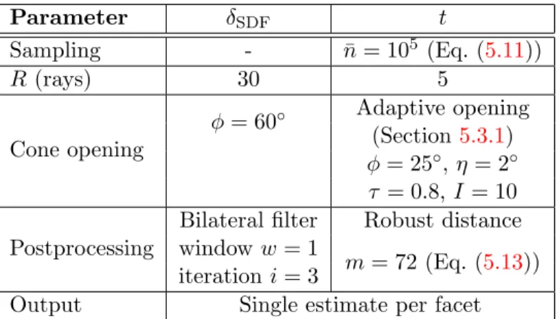
5.3 Parameter settings for the SDF and the thickness estimation . . . 73

7.1 Benchmarked variants of the QP framework and their designation. . . 103

7.2 Median BER against Loop subdivision (1 iteration) for diﬀerent variants of the QP framework. . . 104

(13)

(14)

List of Figures

2-1 Local frame at p with normal section (p, n, t), and the tangent plane spanned by

(t1, t2). . . 10

2-2 Atomic lazy wavelet decomposition . . . 14

2-3 Generic watermarking system with its inputs and outputs . . . 15

2-4 Basic components of a Watermarking System . . . 18

2-5 Schematics for the Scalar Costa Scheme and a binary payload embedding . . . 20

3-1 Summary of the state-of-the-art for 3D Watermarking . . . 43

4-1 Aggregated stability of the local surface area for two neighborhood sizes. . . 50

4-2 Aggregated stability of the Euclidean distance to the center of mass . . . 51

4-3 Aggregated stability of the geodesic distances from a single surface vertex to all the other vertices . . . 52

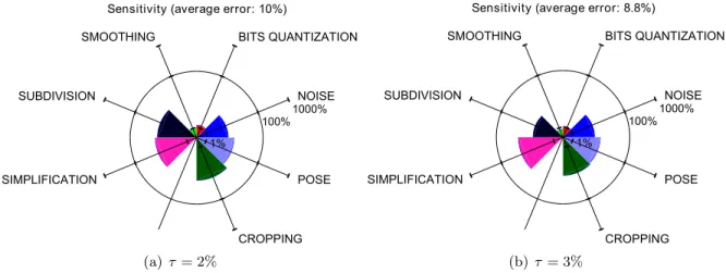
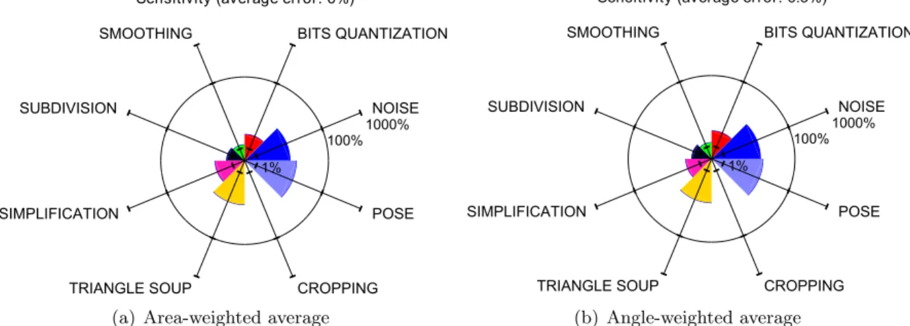
4-4 Aggregated stability of the vertex normal estimates using the area-weighted aver-age4-4(a)and the angle-weighted average 4-4(b). . . 53

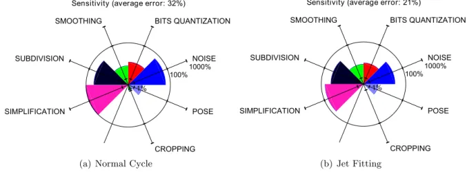
4-5 Aggregated stability of the mean curvature, estimated with the Normal Cycle4-5(a) and a Jet-Fitting4-5(b), using a 3 ring neighborhood. . . 54

4-6 Aggregated stability of the magnitude of the spectral coeﬃcients using a combina-torial Laplacian . . . 55

4-7 Benchmark of the stability of geometric quantities, used to deﬁne a 3D watermark carrier, against multiple attacks . . . 56

5-1 Thickness on an ellipse . . . 61

5-2 Adaptive cone opening to estimate the diameter-based thickness . . . 63

5-3 Half-diameter clouds for the table mesh using two estimation procedures for the diameter . . . 64

5-4 Visibility issue between a boundary point and the half-diameter point cloud . . . 64

5-5 Inﬂuence of the scale-controlling parameter ratio on the thickness . . . 67

5-6 Subset of meshes in a large benchmark database for the thickness estimations . . . . 69

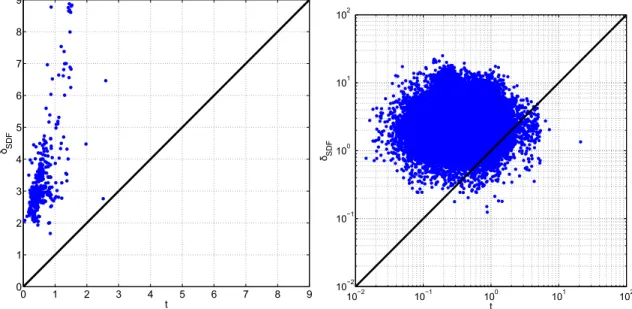
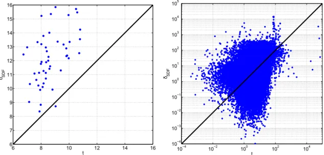
5-7 Accuracy of the thickness estimations for a sphere and a torus . . . 73

5-8 Benchmark of the accuracy of the thickness estimation on ellipsoids . . . 74

5-9 Global instability and local instability of the thickness estimates . . . 75

5-10 Estimated thickness for 3 poses of an elephant mesh . . . 76

5-11 Robustness of the thickness estimates against the pose attack . . . 77

5-12 Global error for the thickness estimate against noise addition . . . 78

5-13 Local error for the thickness estimate against noise addition . . . 79

5-14 Average robustness of the thickness estimate against smoothing . . . 80

(15)

5-16 Average robustness of the thickness estimate against triangle soup . . . 82

5-17 Close-up in the robustness of the thickness estimate against triangle soup . . . 82

5-18 Robustness of the thickness estimate against simpliﬁcation . . . 83

5-19 Close-up in the robustness of the thickness estimate against simpliﬁcation . . . 83

5-20 Robustness of the thickness estimate to remeshing operations . . . 84

5-21 Robustness of the segmentation induced by the thickness estimates, against uniform geometric noise . . . 84

5-22 Variations in the number of segments output from the thickness-based segmentation 85 6-1 Boundary constraints conﬁgurations when deﬁning alternate relocation directions . . 95

7-1 Median RMS vs. median MSDM for the Spread-Transform extension and various embedding strengths . . . 101

7-2 Average BER against noise attacks for diﬀerent spreading lengths . . . 102

7-3 Average BER vs. perceptual embedding distortion for the ST extension of the QP framework at 1% uniform noise addition . . . 103

7-4 Average robustness performance of the integral centroid extension to the QP framework107 7-5 Cumulative distribution of the local MSDM on the dragon mesh for diﬀerent QP variants . . . 108

7-6 Embedding distortion for the fandisk using diﬀerent relocation vector ﬁelds and embedding strength . . . 108

7-7 Average robustness performance of the extensions to the QP framework based on alternate relocation directions and cost functions . . . 109

8-1 Brute-force attack against ϵ on the Bunny mesh . . . 113

8-2 Illustration of the process to remove false positives in the histogram edge detections 114 8-3 Lower bounds Lng and upper-bounds Ung on the secret parameter ∆ . . . 116

8-4 Relative error for the approximations of the secret parameters ˆϵ and ˆ∆ng . . . 117

8-5 Box-plot of the gap magnitudes at the histogram edge locations depending on the cost function . . . 118

8-6 Average absolute correlation between the secret spreading sequence s and its estimate120 8-7 Detail of the watermark carriers and the spreading estimation . . . 121

8-8 Performance of the mutual-information-based estimations of the secret shuﬄing . . . 122

8-9 Performance of the spreading estimations in the presence of an estimated shuﬄing . 123 9-1 Modiﬁed QP-based watermarking system with a cropping-resilient resynchronization component. . . 127

9-2 Quantization grid that determines landmarks . . . 128

9-3 Performance of the blind detection of landmarks on the bunny mesh, measured through ROC curves using increasing landmark strengths α_L . . . 131

9-4 Blind recovery of the center of mass of the bunny . . . . 136

9-5 Steps of the spherical resynchronization approach using a spherical pattern of land-mark points . . . 137

9-6 Benchmark of the robustness of the QP framework with and without a synchroniza-tion component . . . 140

D-1 Some of the meshes in the database. . . 166

(16)

Notations

Vectors are denoted in bold x, matrices in capital bold X. Elements of a matrix X∈ Rn1×n2 _and

a vector x∈ Rn1 _{are denoted X}

i,j, (i, j)∈ J1, n1K × J1, n2K and xi, i∈ J1, n1K.

In R3_{, p indiﬀerently denotes the point or the vector.} _{∥.∥ is the Euclidean norm. |X |}

(respec-tively|x|) is the number of element in the set X , (resp. the vector x). A ‘w’ superscript indicates a watermarked variable.

Main Notations

Notations used throughout the dissertation.

Notation Description

A Total area of the surface mesh

B(g, r) Ball centered at g and of radius r

c Watermark carrier

δa,b Kronecker delta between a and b

E, F Set of mesh edges and facets

In Identity matrix of size n

Ja_b(a0) Jacobian matrix such that its entry J(i,j)(a0) is the ﬁrst derivative at a0 of the ith

component of a with regard to the jth variable in b

L Laplacian matrix derived from a mesh

λ Control parameter for trade-oﬀs

M Mesh, and unless mentioned otherwise, a triangle surface mesh

m, M Watermark payload with antipodal bits, in vector form and as a diagonal matrix

ni, nf, nq Normal vector to the mesh surface at the ith vertex location, on the facet f or at point

q

nv, nf Number of vertices and facets in a mesh

nb Number of payload bits

N1(v),N₁F(v) Sets of, respectively, vertices and facets, in the 1-ring neighborhood of vertex v

p, P Location of a vertex and matrix of all vertex locations in a mesh

q, Q Query point on the mesh surface, and set/matrix of all query points

S(g, r) Sphere centered at g and of radius r

(ux, uy, uz) Basis vectors of the Cartesian coordinates system

vi,V ith mesh vertex and set of mesh vertices

V Volume of the 3D object bounded by the mesh

Thickness Estimation

Notations for Chapter 5.

(17)

aq(f ), aq Local per-facet accuracy of the estimator, and global per-mesh accuracy, over q runs

of the algorithm

b Length of the space diagonal of the bounding box

δSDF Thickness estimation resulting from the SDF procedure

η Aperture closing per iteration

g(f ) Ground-truth estimation of the thickness at a facet f

I Number of iteration for the diameter estimation

Iq_{(f ), I}q _{Local per-facet instability of the estimator and global per-mesh instability, over q runs}

of the algorithm

k Scale of the robust diameter estimate

ns, ¯ns Number of samples in a mesh and normalized number of samples with regard to the

mesh bounding box

ϕ Opening angle of the cone in the diameter estimation

R Number of rays cast in a diameter estimation cone

Rq_F,F′(f ), Rq_F,F′ Local per-facet error of the estimator and global per-mesh error, over q runs of the algorithm

τ Threshold stopping the iterative cone closing

t(q), tk(q) Thickness estimation at query point q (at a scale k when indicated)

w Spatial window of the bilateral smoothing

Watermarking Radial Distances

Notations for Chapters6 to9.

α, α Watermark embedding strength (vector of α)

β Watermark separation oﬀset between bins of the histogram of radial distances

Bi Bin in the histogram of radial distances associated to the ith radial distance (vertex)

δ ¯ρw_i ith unknown in the QP framework corresponding to the normalized relocation of the

associated vertex in the radial direction

δrw

i ith unknown corresponding to the relocation of the associated vertex in the arbitrary direction ui

∆ Histogram step

ϵ Secret parameter in the watermarking system: relative oﬀsets to obfuscate both ends

of a histogram (ϵmin, ϵmax) or dither in QIM.

η Secret seed to generate the secret parameters of a watermark system

g Position of the mesh center of mass

G Set of histogram bins associated to a payload bit

Nj Number of samples in the jth bin of a histogram

L Set of landmark points

m, M Minimum and maximum of the radial distances

nB Number of bins in the histogram of radial distances

ui Relocation direction associated to the ith vertex

ϕi Third spherical coordinate of the ith vertex, with regard to the mesh center of mass

Φ Matrix for the spread-transform projection

Ψ Diagonal matrix of cosines between the radial unit vectors and the arbitrary relocation

directions (scaled by the histogram step ∆)

ρi, ¯ρi, ρi Radial distance from the ith vertex position to the center of mass, normalized radial

distance in [0, 1), and unit radial vector from the center of mass to the vertex

(18)

s, s(η) Spreading sequence, pseudo-randomly generated using the secret seed η

¯_t _{Vector of normalized watermark targets}

θi Second Spherical coordinate of the ith vertex, with regard to the mesh center of mass

ω Cost function to represent the watermark ﬁdelity

w Nonnegative weights

(19)

(20)

Chapter 1

Introduction

1.1 Context

Three-dimensional (3D) models have become ubiquitous in many industrial applications. In movie production, they have been replacing traditional two-dimensional (2D) graphics since the early eighties and the release of Tron (1982) by Walt Disney Pictures. Thanks to ever more powerful animation software products [Aut14] and motion capture systems, animations of 3D models are now routinely used not only in animated movies but also in live-action feature ﬁlms and series as well. The quality and the level of details of 3D models make them more and more indistinguishable from real-life objects. We may for instance be unaware that in the large-scale battles of the Lord of the Rings trilogy, background combatants are 3D models animated through a complex artiﬁcial intelligence system [Reg14].

The rapid dissemination of 3D graphics processing units (GPU) in the mass market around the year 2000 has prompted the video game industry to drift away from 2D, and from pseudo-3D games (simulating 3D using projections of 2D graphics, also known as 2.5D), to fully capable 3D game engines, leading to an abundant use of 3D models. While these 3D assets may be generated by professional game development studios for internal use, new business models for 3D graphics have appeared when companies started producing and brokering this type of content [FC14]. In computational science and engineering, Computer-aided Design (CAD) routinely uses 3D solid modeling for numerical simulations, as it provides the means to cut down research and development costs.

In addition to their professional applications, 3D models are also playing a growing part in user-generated content. For instance, some modern game engines oﬀer the possibility for custom content to be integrated. Creating 3D models for new characters or other game assets has thus grown into a popular activity, supported by dedicated tools [Ble14,Aut14,Epi14] and publications targeting the semi-professional market [Pub13].

The expected booming of 3D printing activities will further expand the importance of 3D models. The accessibility of 3D printers for everyday users is likely to impact consumption scenarios. Contrary to other types of multimedia content, 3D models will turn from cultural and artistic digital products into actual tangible consumer goods. Analysts forecast new trends based on downloading and printing models using on-line databases [WGL+13]. Because 3D models are versatile and will be increasingly available in the mass market, protecting their dissemination and their intellectual property has become a concern.

Aside from patents, trademarks or industrial design rights infringements that always appear with digital creations, copyright infringement is a crucial topic for the entertainment industries [Org08].

(21)

Films and music are notoriously pirated and at the center of a large-scale digital black mar-ket [Ahr06]. Copyright holders have then put a great deal of efforts into tracking the origins of illegal redistributions of their properties. As the complexity and the value of 3D assets increase, similar scenarios are expected to occur with the illicit transmission of copyrighted 3D models. How-ever, because of the ever thinner frontier border between digital models and tangible goods in the real world, this issue is greatly amplified by its potential new impact on merchandising or licensing. Consider a 3D model of the main character of the latest blockbuster. If this model can be illegally downloaded, anybody will be able to manufacture at home some custom goods that bear this character. This is going to affect the sales of, e.g., toys based on this character; if the illegal 3D model is a degraded version of the original, it may also impact the reputation of the copyright holder. For children’s toys, a plurality of norms may also be violated by a counterfeit home-made product, leading to safety problems. Related issues have begun to emerge. In 2012, Games Workshop Limited issued a cease-and-desist notifications for a CAD model and a 3D print based on one of its miniature tank [New12]. In 2013, HBO sent a cease-and-desist against a 3D model for an iPod docking in the shape of the iron throne from the TV show Game of Thrones [Mac14]. In both cases, companies claimed copyright infringement took place. In this context, companies are facing the challenge of identifying if a model is an illegal reproduction of their work or where a counterfeit model originates from.

1.2 Digital Watermarking

Digital watermarking is a technical ﬁeld that provides copyright owners with the means to pro-tect their intellectual property rights. It is a central component of multimedia content propro-tection architectures that complements traditional cryptography [CMB+07]. While cryptography aims at preventing an unauthorized user from accessing a content, watermarking addresses the issues that arise once an authorized user has been granted access, e.g., after the decryption, or if the encryption is broken.

In general, watermarking consists in modifying multimedia content in a robust and imperceptible way in order to hide a secret message. The embedded message, referred to as the watermark payload, can indeed serve as a forensic piece of evidence for ‘traitor tracing’ tasks. Alternatively, it may constitute a proof of ownership in case of litigations. In the former case, authorized users are only given access to a custom copy of valuable 3D assets. Each user would possess an imperceptibly diﬀerent and unique version of the 3D models; users and copies of the original 3D assets thus being one-to-one mapped. If an illegal dissemination of the asset occurs, copyright owners can ﬁnd the leak, as his or her identity is embedded in the pirated publicly-available content. In contrast, in proof of ownership use-cases, the watermark payload corresponds to the identity of the copyright owner. He or she can then successfully prove that a content is his or her own.

Digital watermarking has many other uses for security purposes, e.g., for content tampering detection, and it also has applications outside this scope, for instance in broadcast monitoring. Because of this plurality of applications, digital watermarking systems are usually adapted to meet the speciﬁc requirements of their intended use-cases.

1.3 Problem Statement

From a technical standpoint, all watermarking systems are akin to digital communication systems, where an emitter sends a signal to a receiver through a communication channel. In watermarking,

(22)

the embedder emits a signal, usually encoding a payload, which is carried by the copyrighted con-tent, and then retrieved by the decoder. Both ends of this system are managed by the copyright holders, but the operations applied to the copyrighted content in-between are not controlled: an authorized user is able to arbitrarily modify his or her content. These modiﬁcations need to be han-dled by the watermarking systems, so that the decoder can still retrieve the payload. Watermarking is then characterized by its robustness.

Because increasing the size of the payload usually decreases the robustness, a balance between these two quantities needs to be set. In addition, most people will not accept that the watermarking impacts their everyday use of copyrighted content. The ﬁdelity of the watermark, measuring the amount of change in the watermarked content, further constrains the system. In general, watermarking then faces a complex balance between robustness, ﬁdelity and embedding-rate.

This dissertation focuses on watermarking for 3D models, abbreviated to ‘3D watermarking’, in the context of traitor-tracing. The payload, representing the identity (ID) of a user, needs to be embedded in the model in a very robust and secure manner. Indeed, once it becomes public knowledge that watermarking techniques are being employed, people leaking 3D contents are likely to try and remove the incriminating messages so as to avoid prosecution. The embedding rate of the system then reaches at most a few dozens of bits, and the aforementioned routine watermarking trade-oﬀ focuses on the robustness. These systems are simply referred to as ‘robust watermarking’. In contrast, ‘fragile’ or ‘high-capacity’ 3D watermarking systems focus on increasing the em-bedding rate (‘high-capacity’) or on applications where the constraints on the robustness can be partially lifted, such as content tampering detection (‘fragile’). A plurality of fragile or high-capacity 3D watermarking systems have been proposed instead of robust ones, because providing a high level of robustness in the 3D context yields several scientiﬁc and technical challenges.

1.4 Technical Challenges in Robust 3D Watermarking

Complex issues immediately arise from the very ways 3D models are digitally represented. The robustness of a watermarking system relies in part upon an agreement between the embedder and the decoder on the way they represent the 3D model. When the decoder does not have access to the original non-watermarked 3D object (‘blind watermarking’), achieving such an agreement is actually tough. Nonetheless, providing the decoder with the original object (‘non-blind watermarking’) incurs several practical drawbacks. Issues regarding the representation of 3D models also impact the usefulness of the most successful signal processing tools for robust watermarking, such as the Fourier Transform or the Wavelet Transform. The extensions of these transforms for 3D models are indeed deﬁned in a content-dependent manner. This makes it harder to handle any modiﬁcation of the 3D model between embedding and decoding.

Watermarked 3D models can undergo a variety of possible modiﬁcations. Two types of modi-ﬁcations are very challenging to deal with: the cropping attack and the isometric deformation of the surface, a.k.a., the pose. Both types yield a synchronization problem for watermarking. With cropping, part of the model is deleted, and its value is usually reduced from the point of view of copyright holders. However, even mildly noticeable amounts of cropping may lead to large synchro-nization problems in 3D watermarking. Cropping thus remains a constant issue. Regarding the pose operations, they only occur when animating 3D models. Not all 3D watermarking systems are thus expected to be robust against pose, but it becomes a major concern in contexts where the watermarked 3D assets are parts of animations.

In traitor tracing, the ability for an unauthorized user to access and modify the watermark payload as he or she wishes may have serious legal consequences: the incriminating ID could

(23)

indeed be changed so as to point to another user. No one other than the copyright owner should thus be able to access the embedded ID. This constraint is referred to as a security issue. 3D watermarking research has often either overlooked this issue or used unsound validation methods. On the opposite, thorough theoretical analyses have been undertaken to assess the watermark security in other types of content.

As copyright holders may use their 3D assets to advertise their work, they expect robust water-marking systems to also preserve the visual appearance of the 3D models, i.e. to always achieve a given level of fidelity. There is however no definite way for measuring the perceptual impact of an embedding in 3D graphics. Perceptually-correlated distortion metrics are still being investigated. The few existing solutions all present some shortcomings. Their adoption by the watermarking community is limited, which has hindered research, as different watermarking systems are not aligned with regard to the same distortion metrics.

At last, many 3D automated operations (algorithms, procedures) have some requirements on their 3D inputs. These requirements are often not met in real-life, and 3D objects often need to be repaired before being processed, for instance by removing some defects. Most databases that were not created for research purposes thus cannot be straightforwardly used to perform large benchmarking campaigns. Unlike in audio and images, only small scale 3D watermarking benchmarks are feasible.

1.5 Outline

Chapter 2 provides a more technical introduction to the 3D watermarking domain and some key background notions on 3D objects processing and watermarking. The remaining chapters are then grouped in two parts.

Part one of this dissertation focuses on content adaptation transforms for 3D watermarking. The main state-of-the-art robust watermarking systems, classiﬁed according to their adaptation transforms, are reviewed in Chapter 3. A benchmark of some of the most common adaptation transforms is reported in Chapter 4. Finally, Chapter5 investigates a novel extraction transform, based on the thickness of 3D objects, which exhibits promising properties against pose operations. Its performance is thoroughly tested.

Part two of this dissertation focuses on enhancing and extending a constraint optimization formulation for 3D watermarking, to create a modular and versatile framework for robust water-marking systems. Chapter6details several extensions to improve the robustness and the ﬁdelity of the original watermarking formulation. These extensions are then experimentally benchmarked in Chapter7. Chapter8takes a closer look at the security of the watermarking framework by describ-ing a series of attacks and counter-measures. Finally, the speciﬁc issue of croppdescrib-ing is addressed in Chapter 9, with a novel resynchronization approach that is added to the framework.

Chapter 10 summarizes the main results presented in this dissertation. The original contri-butions of this work to the 3D watermarking ﬁeld are emphasized, and stimulating directions for future research are listed.

1.6 List of publications

(24)

International Publications

• Anti-Cropping Blind Resynchronization for 3D Watermarking. Xavier ROLLAND-NEVIÈRE, Gwenaël DO ËRR, Pierre ALLIEZ. Submission to ICASSP, 2015.

• Security Analysis of Radial-based 3D Watermarking Systems. Xavier ROLLAND-NEVIÈRE, Gwenaël DO ËRR, Pierre ALLIEZ. Proceedings of the IEEE Workshop on Information Foren-sics and Security, 2014 [to appear].

• Spread-Transform and Roughness-based Shaping to improve 3D Watermarking based on Quadratic Programming. Xavier ROLLAND-NEVI `ERE, Gwena¨el DO ¨ERR, Pierre ALLIEZ. Proceed-ings of the IEEE International Conference on Image Processing, 2014 [to appear].

• Triangle Surface Mesh Watermarking based on a Constrained Optimization Framework. Xavier ROLLAND-NEVI ÈRE, Gwenaël DO ËRR, Pierre ALLIEZ. IEEE Transactions on Informa-tion Forensics and Security, vol. 9, no 9, September 2014, pp. 1491-1501.

• Robust Diameter-based thickness estimation for 3D objects. Xavier ROLLAND-NEVIÈRE, Gwenaël DO ËRR, Pierre ALLIEZ. Graphical Models, vol. 75, no 6, November 2013, pp. 279-296.

Patents Applications

• Generalized Quadratic Programming Framework for 3D Watermarking. Xavier ROLLAND-NEVI ÈRE, Gwenaël DO ËRR, Pierre ALLIEZ.

• Thickness-based 3D Watermarking. Xavier ROLLAND-NEVIÈRE, Gwenaël DOËRR, Pierre ALLIEZ.

• Method for introducing watermark feature points on a surface mesh. Xavier ROLLAND-NEVI ÈRE, Gwenaël DO ËRR, Pierre ALLIEZ.

• Method for using landmark points as a resynchronization mechanism for 3D watermarking. Xavier ROLLAND-NEVI ÈRE, Gwenaël DO ËRR, Pierre ALLIEZ.

(25)

(26)

Chapter 2

Background Notions for 3D

Watermarking

3D watermarking is a subfield of research whose foundations are built on both the digital water-marking and the geometry processing domains. Some necessary background information from these areas is reviewed in the first two sections of this chapter. In Section2.3, the recent findings on the assessment of 3D mesh distortion are summarized. Research carried out in this domain is indeed especially relevant to 3D watermarking; the state-of-the-art review presented in Chapter3 heavily relies on all the notions introduced next.

2.1 Triangle Mesh Processing

This section is dedicated to introducing some basic concepts relating to 3D objects. A few advanced topics for mesh processing, routinely used in the context of 3D watermarking, are eventually re-viewed.

2.1.1 Triangle Mesh Definition

Representation of 3D Objects

Creating and processing the geometry of three-dimensional (3D) data is one of the main subﬁeld of research in computer graphics. In this context, 3D data are 3D objects that can be represented in many ways, using voxels, point-clouds, splines, volumetric or polygonal meshes. . . Some of these representations focus on the description of the surface boundary of a 3D object, formally deﬁned as “an orientable continuous 2D manifold embedded inR3” [BKP+10]. The parametric representation of a surface is a mapping f from Ω⊂ R2 to f (Ω)⊂ R3.

The definition of a surface only allows for 3D objects to be non-degenerate 3D solids, i.e. both watertight and nowhere infinitely thin objects. Still, practical computer graphics applications are usually able to handle surfaces with boundaries. These correspond to surfaces with holes that can be filled, so as to turn them into proper orientable continuous 2D manifold.

Surface Mesh for 3D objects

Since surfaces are continuous, their digital representations are only discrete approximations, a.k.a. samplings. One of the most popular digital representation is a piecewise linear approximation in the form of a polygon surface mesh. Formally, a polygon surface mesh M is deﬁned by its

(27)

geometry and connectivity. The latter is a graph structure. Its set of vertices and edges are respectivelyV = {vi, i∈ J1, |V|K}, and E = {e(i,j), (i, j)∈ J1, |V|K2}. The geometry, also referred to

as the ‘embedding’ of the 2D surface in R3, is deﬁned by mapping a vertex vi to a point pi ∈ R3.

P∈ R3×nv_{, referred to as the ‘vertex positions’, denotes the matrix representing the concatenation} of all vertex positions. It corresponds to approximation of the underlying surface boundary of the 3D object, and constitutes an irregularly sampled signal. Unless mentioned otherwise, nv always

denotes the number of vertices in mesh.

2-manifold surfaces are represented with 2-manifold polygonal surface meshes, which are char-acterized by the fact that: (i) they do not present any self-intersection, and (ii) all their edges are exactly shared by two faces of their graph (or at least one face for a 2-manifold with boundaries). An alternate characterization of a 2-manifold surface mesh is that the local neighborhood of all ver-tices is homeomorphic to a disk (or half a disk for a 2-manifold with boundaries). Data-structures have been developed for these meshes to minimize storage and optimize neighborhood searches and traversals of the mesh [FGK+98]. In this context, the set of polygon faces F = {fi, i∈ J1, |F|K} is

often used instead of E to describe the connectivity information. nf henceforth denotes|F|.

Triangle Surface Mesh

A sub-case of polygonal surface meshes are triangle surface meshes, where all polygons are triangles. 3D watermarking mainly focuses on triangle surface meshes, which will subsequently be simply referred to as ‘meshes’. The motivation for choosing triangles as primitives is that: (i) polygons can always be partitioned into triangles, and (ii) vertices in arbitrary polygon facets may neither be coplanar nor convex inR3. Note that most of the aforementioned eﬃcient data-structures also handle some degenerate meshes, such as ones with non-manifold vertices incident to two distinct triangle fans (sets of connected triangles sharing one central vertex).

Neighborhood and Regularity

The one-ring neighborhood of a vertex vi, also referred to as its star neighborhood, is the setN1(vi),

formed by the vertices which are linked to viby a mesh edge, i.e. : {vj ∈ V | e(i,j)∈ E}. The n-ring

neighborhood of a vertex is then recursively deﬁned from the 1 ring. This neighborhood deﬁnition is commonly used for its simplicity as a connectivity-based only quantity. A neighborhood search then reduces to a graph search inE, and does not involve any computation on the geometric information inP, which are only sampling approximations.

|N1(vi)| is the valence of vi. Triangle meshes are labeled as regular when the valence of all the

vertices is exactly six. When a mesh is only piecewise regular, in other words, almost everywhere regular, it is labeled as semi-regular. Otherwise, meshes are labeled as irregular.

The triangle facets in the one ring neighborhood of a vertex vi, denoted by N1F(vi), are the

facets of F in which vi is a vertex.

Smooth Surface Mesh Representation

Smooth surfaces are characterized by: (i) their parametric representation maps f are Ck contin-uous (k≥ 2), and (ii) the partial derivatives of f do not vanish. Although the mesh geometry maps vertices to discrete points, a mesh surface is still continuous. But since it is only piecewise linearly continuous, most of the quantities that are deﬁned on a smooth surface boundary of a 3D object cannot be straightforwardly extended to meshes. A ﬁrst challenge in mesh processing is to approximate these quantities.

(28)

Moreover, in computer graphics, the surfaces represented via meshes are expected to be almost everywhere smooth, except in a ﬁnite number of locations called ‘sharp features’. These are often found in mechanical objects, e.g. the fandisk mesh. Dealing with sharp features is another major challenge in geometry processing and in 3D watermarking.

Other Types of Information

Much additional information can be added to a mesh such as colors and normal directions for vertices, labels to create groups of faces, or texture maps, etc. This information enriches the visual appearance when rendering the mesh on screen. Because this information may be straightforwardly removed from a mesh ﬁle (for example, in an Object File Format (OFF), colors are stored in optional dedicated columns), robust 3D watermarking research generally does not take them into account.

All the meshes considered hereafter are solely deﬁned through their vertex positions P, and their vertices V linked to form the triangle facets F. TableD.1 lists the experimental database of meshes that is mainly used in the following, as well as some of their speciﬁcities, such as defects, complexity or type.

To conclude this series of deﬁnition, meshes and surfaces described above are sometimes referred to as ‘static’, as opposed to the ‘dynamic’ ones that are used in 3D animations. In this dissertation, we only deal with statically deﬁned objects.

2.1.2 Mesh Processing

Intrinsic vs. Extrinsic Quantities

The first fundamental form at a point p on a surface is defined as the dot product of two tangent vectors. It is canonically written as a two-by-two symmetric matrix whose coefficients are derived from the parameterization of the surface. It fully characterizes the metric properties of the surface, such as the area of a surface patch, or the geodesic distance between two points.

The first fundamental form is essential to distinguish between intrinsic and extrinsic quantities measured on a smooth surface. Intrinsic quantities are measured inside the surface. Intuitively, they could be computed by entities evolving on the surface, much like humans on the Earth. More formally, they are expressed solely in terms of the coefficient of the first fundamental form and do not depend on the embedding of the surface in R3. This is the case for the aforementioned surface area, or geodesic distances. In contrast, extrinsic quantities, such as the Euclidean distance, depend on the actual embedding.

Using intrinsic or extrinsic quantities directly impacts the properties of a watermarking system, such as its robustness (see Section2.2.2) or its complexity.

Mesh Curvatures

One of the key notion in diﬀerential geometry is the curvature of a smooth surface. In R2, the curvature of a smooth curve intuitively measures how it deviates from a straight line, and is formally deﬁned with the derivative of the tangent vector to the curve. For surfaces, given a tangent vector

t∈ R3 to the surface at p, the curvature κ(p, t) is the curvature of the curve deﬁned by the intersection between the surface and the plane spanned by (p, n, t), where n∈ R3 is the normal to the surface at p (see Figure 2-1.

The principal curvatures (κmin(p), κmax(p)) are the minimum and maximum values over the

tangent directions of κ at p; the principal directions are the tangent vectors associated to the prin-cipal curvatures. These speciﬁc curvatures, as well as the mean curvature κmean= 1₂(κmin+ κmax)

(29)

Figure 2-1: Local frame at p with normal section (p, n, t), and the tangent plane spanned by (t1, t2).

and the Gaussian curvature, κG= κminκmax are used to characterize and classify the local shape

of smooth surfaces. While the mean curvature is extrinsic, the Gaussian curvature is intrinsic (Theorema Egregium).

Extending the computation of surface curvatures to meshes, which are only piecewise linear, has been an active field of research. Curvatures are extensively used in geometry processing. For instance, in remeshing applications1, curvatures play a key part in defining non-uniform and locally adapted efficient sampling density [ACSD+03]. In 3D watermarking, the estimation of the principal curvatures has multiple applications, such as distortion metric (see Section2.3) and synchronization mechanism definitions [AM05].

Two main strategies to compute the principal curvatures and the principal directions at a query point have been investigated. A first solution is to fit an analytic surface to a local patch around the point. For analytic surfaces with polynomial expressions, the curvatures can be written in closed-form depending on the polynomial parameters. This leads to an efficient curvature approximation, depending on the quality of the fitting [CP03]. A second category of approaches is built on the theory of normal cycles and its extension to polyhedral surfaces [CSM03]. In essence, the curvatures are computed as a weighted average of the signed dihedral angle of edges around p. In Chapter4, we investigate the use of both types of curvature estimators for robust watermarking purposes.

Rigid Mesh Alignment

Several mechanisms to canonically normalize a mesh have been proposed in the mesh process-ing literature. In 3D watermarkprocess-ing, a Principal Component Analysis (PCA)-based normalization mechanism [ZC01] and an Iterative Closest Point (ICP) [BM92]-based normalization mechanism have been widely adopted.

The ICP is inherently restricted to the case where the mesh to be normalized is associated with another mesh (for instance, in a non-blind watermarking system, as deﬁned in Section2.2.1). Its basic steps consists of (i) matching a series of points between an original and a query mesh, (ii) minimizing a Mean Square Error (MSE) cost function that models the mesh alteration with a rotation/translation, (iii) apply the estimated transform to the query mesh, and (iv) iterate the previous steps until some minimum cost threshold is reached.

The major advantage of PCA-based normalization over the ICP is that there is no need for a reference mesh (it can thus be used in blind watermarking, and the normalization is applied at both ends of the watermarking system, see Section2.2.1). Its main steps are: (i) translating the mesh so that its center of mass is at the origin; (ii) scaling the mesh uniformly so that it is bounded within

1

(30)

e.g. a unit-sphere2; (iii) performing a PCA of the mesh and aligning the principal directions with the coordinate axes; and (iv) selecting from the possible remaining mesh configurations the one in which some high order terms in the vertex positions are positive. For symmetric configurations, e.g. a spherical mesh, these last two steps may however be ill-defined, as the principal directions are ambiguous. The covariance matrix in the PCA is computed by summing over the mesh second degree terms, such as x2_i, xiyi. . . The high order terms are the summation over the mesh of some

third degree expressions in the vertex coordinates, such as x3_i, y_i3.

In watermarking, both the ICP and the PCA provide robustness against rigid transforms (and scaling).

Spectral Analysis

Frequency analysis (also called Fourier analysis) is a powerful and versatile family of tools for audio, image and video processing. Signal processing algorithms heavily rely on the Discrete Fourier Transform (DFT) or the Discrete Cosine Transform (DCT), and their efficient implementations with, e.g., the Fast Fourier Transform (FFT), to compute a spectral representation of a media. Their applications range from denoising to fingerprinting, watermarking, or compression. A large body of research has thus focused on extending these spectral analysis tools to meshes [ZVKD10]. In 1D, the fundamental transform to compute the spectrum of a digital signal in Rn is the DFT. It consists in projecting the signal onto a series of orthogonal and discretized basis functions, a.k.a. harmonics, which spans the spectral domain. These harmonics are the eigenvectors of the 1D discrete Laplace Operator, and correspond to a series of pairs of cosines and sines, sampled at the signal frequency. The frequencies of each harmonic pair is the square root of the associated eigenvalue of the discrete operator3. The projection results in two series of scalar coefficients, defined as the DFT of the signal, a.k.a. its spectral representation. To compute the spectral representation of a mesh, one needs to extend the definition of the discrete Laplace Operator to surface meshes embedded inR3.

This extension involves however a complex approximation problem, that was shown to be a ‘no-free lunch’ one [WMKG07]. It is theoretically impossible to define a Laplace Operator for meshes that match all essential properties of the continuous Laplace Operator in lower dimensions. Some of these properties are however instrumental for spectral analysis. Researchers have thus proposed a variety of Laplacian discretizations for meshes, which all present different benefits and limitations, depending on which ones of the antagonistic properties are preserved.

Notions 1D discrete signals Mesh

Laplace Operator Discrete 1D Laplace Operator Laplacian Matrix L Harmonics Discrete cosines/sines Eigenvectors of L (bases) Frequencies Cosine/sines frequencies (Square root) Eigenvalues of L Spectral Coeﬃcients Cosine/Sine amplitudes 3D projections of P on the bases Table 2.1: Equivalences between the routine 1D spectral concepts and the spectral analysis for meshes.

Table 2.1lists the analogous concepts between the 1D discrete spectral analysis and the mesh spectral analysis. Assuming that the Laplacian matrix L∈ Rnv×nv _{is a real symmetric positive}

2

This is therefore not a rigid mesh alignment operation.

3_{The operator is positive semi-deﬁnite and the multiplicity of all but the null eigenvalue (the DC component) is}

(31)

semi-deﬁnite, its eigenvectors hk∈ Rnv _(k∈ J1, n

vK) are orthogonal and form the discretized basis

functions for the spectral domain. Their associated eigenvalues λ2

k are the squared frequencies of the mesh spectrum. The

projec-tion of the discrete geometry signal onto the kth eigenvector yields a spectral coeﬃcient (triplet) associated to the frequency λk, denoted by Xk, Yk, Zk)4:

[Xk, Yk, Zk]T = Phk. (2.1)

The amplitude of the mesh spectrum at the λkfrequency is the magnitude of the spectral coeﬃcient.

Finally, reconstructing a mesh from its spectral representation amounts to projecting back the spectral coeﬃcients, with:

PT =

nv ∑

k=1

hk[Xk, Yk, Zk] (2.2)

For watermarking purposes, two discretizations have been mainly used: the combinatorial Lapla-cian and the Manifold Harmonics.

Combinatorial Laplacian The combinatorial Laplacian is only based on the mesh connectivity and has been introduced for compression purposes [KG00a]. It is equivalent to a uniform discretiza-tion of the continuous Laplacian for 2D surfaces. Because the connectivity represents a graph, some of the properties of this discretization have been studied in Spectral Graph Theory.

Formally, the Laplacian L is deﬁned with:

L = D− A, (2.3)

where A is the adjacency matrix, whose entry A(i,j)is equal to 1 when vi and vj are connected by

an edge, and null otherwise. D is a diagonal matrix whose entry D_(i,i) is equal to the valence of vi.

Since L is a real sparse positive semi-deﬁnite matrix, eﬃcient algorithms can be used to extract some of its eigenvectors. Using the combinatorial Laplacian5_{, researchers have analyzed the impact}

of quantizing the spectral coeﬃcients in diﬀerent spectrum ranges, e.g., low-frequencies vs. high-frequencies, and found that the Human Visual System (HVS) is less sensitive to perturbations in the lower frequencies [SCOT03]. In 3D watermarking, this observation has led to a thread of research (see Section3.3).

The main limitation of this discretization is that none of the mesh geometry is taken into account. This is however considered to be one interesting property for a discretization of the Laplacian Operator [WMKG07].

Manifold Harmonics Manifold Harmonics [VL08] correspond to a more complex discretization approach. Applying either Discrete Exterior Calculus or Finite Element Method6to the deﬁnition of the operator in the continuous setting, i.e. the divergence of the gradient, leads to an approximation of the Laplacian as a non-symmetric matrix: L =−D−1Q. Q∈ Rnv×nv _{is a matrix of cotangent}

4

This deﬁnition implicitly assumes a one-to-one correspondence between spectral coeﬃcients and eigenvalues, which does not exist in the aforementioned 1D case, as all but one eigen subspace have dimension 2. This comes from the choice of boundary conditions: for the DFT, periodic boundaries are set; for the DCT, Neumann boundary conditions are used. In the latter cases, the multiplicity of the eigenvalues reduces to 1.

5_{More precisely, a full rank version thanks to the addition of as many constraints, i.e. rows, as the number of}

connected components of the mesh, since it can be shown that this number equals the order of the null eigenvalue of the Laplacian matrix.

6

(32)

weights (the stiﬀness matrix) and D is a diagonal matrix of triangle facet areas (the mass matrix). Their entries are:

Qi,j =

1 2 (

cot(βi,j) + cot(βi,j′ )

) , (2.4) Qi,i = − nv ∑ j=1 Qi,j, (2.5) Di,i = 1 3 ∑ f∈N₁F(vi) |f|. (2.6)

(βi,j, β′i,j) are the two angles opposite the edge that connects vi and vj, |f| is the area of facet f

and N₁F(vi) denotes the set of facets adjacent to vi.

Because L is not symmetric, its eigenvectors are no longer orthogonal inRnv_{. However, this issue} can be addressed by rewriting the eigen-decomposition of L as a generalized eigenvalue problem:

− Qh = λDh. (2.7)

(λ, h) is an eigen-pair of eigenvalue and eigenvector. Since (i) both Q and D are symmetric, and (ii) D is positive-deﬁnite, it follows that: (i) there still exists a basis of (generalized) eigenvectors hk which span the spectral domain, (ii) the associated eigenvalues are real, and (iii) the eigenvectors are D-orthogonal, e.g. h1Dh2 = 0.

In summary, spectral coefficients, in the manifold harmonics case, are defined with the following procedure. First, the generalized eigenvalue problem in Eq. (2.7) is solved. It provides the basis functions hk and the associated frequencies that define the mesh spectral domain. To ensure that the basis is orthonormal with regard to the scalar product induced by D, the basis functions are unitary normalized with:

¯ hk = 1 ∥hk∥ D hk= √ 1 (hk₎T _Dhk hk. (2.8)

Then, the geometry signal P is projected onto the basis using the modiﬁed scalar product, resulting in the triplet of spectral coeﬃcients:

[Xk, Yk, Zk]T = PD¯hk. (2.9)

The inverse transform is identical to the previously deﬁned one:

PT = nv ∑ k=1 ¯ hk[Xk, Yk, Zk] (2.10)

Discussion All the spectral decomposition tools result in a set of orthonormal basis vectors, a.k.a. the harmonics hk_{, that spans the spectral domain.} _{Thanks to this property, practical}

applications, such as watermarking, compression or ﬁngerprinting, do not need to fully perform the eigen-decomposition nor estimate all the eigenvectors. One usually only computes speciﬁc sub-bands of the spectrum, making this tool applicable to medium-sized meshes, with e.g. more than 106vertices. For instance, as most of the energy of the geometric signal lies within the low-frequency part of the spectrum (eigenvectors associated with the smallest eigenvalues), only this sub-band is commonly extracted. Nevertheless, performing a limited eigen-decomposition of very large sparse matrices still presents practical challenges, especially on consumer-grade hardware.

(33)

A crucial theoretical drawback of all the spectral decomposition approaches is that the har-monics, on which the mesh geometry is projected, are derived from a discretized Laplacian that is itself content-dependent. This stems from the very nature of the mesh representation, as an irregular sampling of 2D data in a 3D space. In other words, unlike 1D or 2D, where the canonical cosines and sines are used, the basis functions are themselves content-dependent. This gives rise to a number of issues, especially in the watermarking context.

Multiresolution Analysis

Multiresolution analysis is a processing tool that consists in iteratively decomposing a signal into a coarse base approximation and a series of reﬁning details that can be further decomposed. It was ﬁrst introduced in the context of meshes [LDW94] to compute a level-of-detail hierarchy, i.e. multiple representations of the same input with increasing details. It has found applications in various domains [Gar99], such as multiresolution editing [ZSS97], progressive rendering, compres-sion [EDD+95] and watermarking.

The initial approach is an extension of the wavelet transform for semi-regular meshes with the so-called ‘lazy wavelet decomposition’. As depicted in Figure2-2, the atomic decomposition operation transforms a group of four triangles into a coarse signal and a refinement signal. The former is a single triangle face that preserves three of the original vertices; the latter is a set of three prediction error vectors in R3, a.k.a. the wavelet coefficients, associated to the edges of the coarse triangle. Each one translates the mid-point of its associated edge to the position of the original vertex that has been removed. This subdivision and correction operation can be equivalently formulated in a series of filter banks. Applying the filters to a mesh creates a series of meshes ranging from detailed to coarse, and a series of associated 3D refinement details. The coarsest mesh is referred to as the base mesh.

Figure 2-2: Lazy-wavelet decomposition on a 4-1 subdivision mesh. The four facets are decomposed into two parts: (i) vertices v2, v4 and v6 form the coarse mesh, (ii) vertices v1, v3and v5 are labeled

as details, and encoded with the wavelet coefficients, i.e. translation vectors from the midpoint of the edges of the coarse mesh.

Lazy wavelets are a particular instance of a broader class of decompositions labeled as ‘lifting schemes’ [Swe96], that uses linear interpolation instead of direct subsampling. In general, multireso-lution analysis presents a low complexity, especially with regard to the existing spectral transforms, and can be applied to meshes with arbitrary topology. However, the need for semi-regularity is

(34)

in practice cumbersome. Researchers have explored two strategies to extend multiresolution to meshes with arbitrary connectivity.

A first solution is to define a remeshing procedure that automatically approximates an initial mesh with another that has subdivision connectivity [EDD+95]. This approach enables leveraging the large body of literature on remeshing and also keeps the efficient, but limited, multiresolution tool. However, the remeshing operation may be computationally costly.

Another solution is to directly extend the limited multi-resolution tool to meshes with arbitrary connectivity [VP04]. In this case, the atomic decomposition step is first modified by adapting the subdivision scheme to the local connectivity configuration. Instead of only allowing 4-1 subdivisions, codebooks with series of possible simplification operations are used. Second, the filter banks to compute the coarse and refined geometry information are modified to account for the changes in the subdivision procedure. On the one hand, this solution does not require a costly remeshing preprocess, and is fully capable of handling arbitrary connectivity. On the other hand, the filter bank analysis becomes more complex, and the multiresolution decomposition depends on additional parameters.

2.2 Notions of Watermarking

Digital watermarking is deﬁned as “the practice of imperceptibly altering a Work to embed a message about that Work” [CMB+07]. A ‘Work’, also called ‘content’ is a multimedia host signal, which can be an image, a video, or a mesh.

2.2.1 Properties of Watermarking Systems

The basic functional model for watermarking, depicted in Figure 2-3, is made-up of three main components: the embedder and the decoder (also called the ‘detector’), which are placed at both ends of the communication channel. Thanks to this representation, a watermarking system can be described with similar concepts as the ones used in communication systems.

A watermark embedder requires three inputs: a content, a payload and a secret key. It outputs the watermarked media. A detector requires at least two inputs: a content and a secret key. It outputs the payload (if any) estimated from the content.

embedder communication channel decoder

side-information (metadata) payload

decoded payload

secret key secret key

Figure 2-3: Generic watermarking system with its inputs and outputs

3D watermarking can be defined at a high-level as the subfield where the input content for the embedder is a 3D asset. In most cases, two main assumptions are added. First, the 3D asset input in the embedder is represented by a mesh, as defined in Section 2.1. This is motivated by the popularity and versatility of triangle surface mesh representations. Second, the decoder only processes 3D assets, and in most cases, meshes. This restricts the use-cases of 3D watermarking to

(35)

applications where 3D assets are not converted to 2D content within the communication channel. This would occur if a decoder were to extract the payload from a rendered image of a mesh. Such a scenario is considered to be out of scope of current watermarking research, and only a handful of attempts have been made to lift this second restriction [BD06].

Capacity

As in other communication systems, the watermark payload, a.k.a. the message, is always assumed to be a series of independent and identically distributed (i.i.d.) random antipodal bits, denoted by m∈ {−1, 1}nb_{). The payload size n}

b depends on the target applications, and characterizes the

embedding rate of a watermarking system, expressed in bits per mesh. The capacity of a communi-cation channel is the upper-bound on the information rate that can be correctly conveyed through the channel. Following common practice in 3D watermarking, ‘capacity’, in this dissertation, refers to the embedding rate of the system.

For robust watermarking applications, such as traitor-tracing, common capacities range from a few dozen bits to a few hundred bits, with nb often chosen among{16, 32, 64}. In 3D watermarking,

some systems are referred to as ‘high-capacity’ watermark, as they focus on providing a maximum capacity, usually around 1 bit per vertex.

Robustness

The communication channel models all the transformations, a.k.a attacks, undergone by a water-marked content before being processed by the decoder. Section 4.2.1 details a list of attacks on meshes taken into account when designing robust 3D watermarking systems. Because of these alterations, the decoded payload ˆm may not be the same as the embedded one. In this context,

the robustness of the system measures how close ˆm is from m. The assessment metric is the Bit

Error Rate (BER).

BER(m, ˆm) = 1− 1 nb nb ∑ i=1 δ(mi, ˆmi), (2.11) where δ_(m_i_{, ˆ}_m_i₎ is the Kronecker delta.

Since the BER measures the ratio of erroneous estimated bits over the total number of trans-mitted bits, it is suitable for multi-bits watermarking. In the speciﬁc case where nb = 0, also called

‘zero-bit watermarking’, the decoder outputs a binary decision on whether or not a content is wa-termarked. The Receiver Operating Characteristic (ROC) or the Area Under the Curve (AUC), designed to measure the performance of binary classiﬁers, are then used to assess the robustness. These metrics provide access to soft information; intuitively, they indicate the conﬁdence of the decoder in its decision. In practice, zero-bit watermarking systems may be implemented using a non-null nb, but the decoder only outputs a binary decision, indicating whether or not the input

has been watermarked.

Blind watermarking

As depicted in Figure 2-3, watermarking systems may also rely on metadata (sometimes referred to as ‘side information’) being directly transmitted from the embedder to the decoder. For water-marking purposes, this content-dependent information is always assumed to be unaltered. In other words, the metadata output by the decoder, for some watermarked content, is identical to the one input to the decoder when decoding this watermarked content.