HAL Id: hal-02306566
https://hal.inria.fr/hal-02306566
Submitted on 11 Oct 2019
HAL is a multi-disciplinary open access
archive for the deposit and dissemination of
sci-entific research documents, whether they are
pub-lished or not. The documents may come from
teaching and research institutions in France or
abroad, or from public or private research centers.
L’archive ouverte pluridisciplinaire HAL, est
destinée au dépôt et à la diffusion de documents
scientifiques de niveau recherche, publiés ou non,
émanant des établissements d’enseignement et de
recherche français ou étrangers, des laboratoires
publics ou privés.
Directed Acyclic Graphs
Julien Herrmann, Yusuf Özkaya, Bora Uçar, Kamer Kaya, Umit Catalyurek
To cite this version:
Julien Herrmann, Yusuf Özkaya, Bora Uçar, Kamer Kaya, Umit Catalyurek. Multilevel Algorithms
for Acyclic Partitioning of Directed Acyclic Graphs. SIAM Journal on Scientific Computing, Society
for Industrial and Applied Mathematics, 2019, 41 (4), pp.A2117-A2145. �10.1137/18M1176865�.
�hal-02306566�
DIRECTED ACYCLIC GRAPHS 2
JULIEN HERRMANN†, M. YUSUF ¨OZKAYA†, BORA UC¸ AR‡, 3
KAMER KAYA§, AND UMIT V. C¨ ¸ ATALY ¨UREK† 4
Abstract. We investigate the problem of partitioning the vertices of a directed acyclic graph
5
into a given number of parts. The objective function is to minimize the number or the total weight
6
of the edges having end points in different parts, which is also known as edge cut. The standard load
7
balancing constraint of having an equitable partition of the vertices among the parts should be met.
8
Furthermore, the partition is required to be acyclic, i.e., the inter-part edges between the vertices
9
from different parts should preserve an acyclic dependency structure among the parts. In this work,
10
we adopt the multilevel approach with coarsening, initial partitioning, and refinement phases for
11
acyclic partitioning of directed acyclic graphs. We focus on two-way partitioning (sometimes called
12
bisection), as this scheme can be used in a recursive way for multi-way partitioning. To ensure
13
the acyclicity of the partition at all times, we propose novel and efficient coarsening and refinement
14
heuristics. The quality of the computed acyclic partitions is assessed by computing the edge cut.
15
We also propose effective ways to use the standard undirected graph partitioning methods in our
16
multilevel scheme. We perform a large set of experiments on a dataset consisting of (i) graphs
17
coming from an application and (ii) some others corresponding to matrices from a public collection.
18
We report significant improvements compared to the current state of the art.
19
Key words. directed graph, acyclic partitioning, multilevel partitioning
20
AMS subject classifications. 05C70, 05C85, 68R10, 68W05
21
1. Introduction. The standard graph partitioning (GP) problem asks for a 22
partition of the vertices of an undirected graph into a number of parts. The objective 23
and the constraint of this well-known problem are to minimize the number of edges 24
having vertices in two different parts and to equitably partition the vertices among 25
the parts. The GP problem is NP-complete [13, ND14]. We investigate a variant of 26
this problem, called acyclic partitioning, for directed acyclic graphs. In this variant, 27
we have one more constraint: the partition should be acyclic. In other words, for a 28
suitable numbering of the parts, all edges should be directed from a vertex in a part 29
p to another vertex in a part q where p ≤ q. 30
The directed acyclic graph partitioning (DAGP) problem arises in many appli-31
cations. The stated variant of the DAGP problem arises in exposing parallelism in 32
automatic differentiation [6, Ch.9], and particularly in the computation of the Newton 33
step for solving nonlinear systems [4, 5]. The DAGP problem with some additional 34
constraints is used to reason about the parallel data movement complexity and to dy-35
namically analyze the data locality potential [10, 11]. Other important applications 36
of the DAGP problem include (i) fusing loops for improving temporal locality, and en-37
abling streaming and array contractions in runtime systems [19], such as Bohrium [20]; 38
(ii) analysis of cache efficient execution of streaming applications on uniprocessors [1]; 39
(iii) a number of circuit design applications in which the signal directions impose 40
acyclic partitioning requirement [7,29]. 41
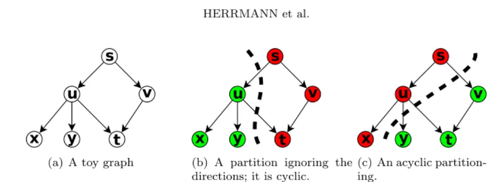
Let us consider a toy example shown inFigure 1.1(a). A partition of the vertices 42
∗A preliminary version appeared in CCGRID’17 [15].
†School of Computational Science and Engineering, Georgia Institute of Technology, Atlanta, Georgia 30332–0250,[email protected], [email protected], [email protected].
‡CNRS and LIP (UMR5668 Universit´e de Lyon - CNRS - ENS Lyon - Inria - UCBL 1), 46, all´ee d’Italie, ENS Lyon, 69364, France,[email protected].
§Sabancı University, Istanbul, Turkey,[email protected]. 1
(a) A toy graph (b) A partition ignoring the directions; it is cyclic.
(c) An acyclic partition-ing.
Fig. 1.1: a) A toy example with six tasks and six dependencies, b) a non-acyclic partitioning when edges are oriented, c) an acyclic partitioning of the same directed graph.
of this graph is shown inFigure 1.1(b)with a dashed curve. Since there is a cut edge 43
from s to u and another from u to t, the partition is cyclic, and is not acceptable. An 44
acyclic partition is shown inFigure 1.1(c), where all the cut edges are from one part 45
to the other. 46
We adopt the multilevel partitioning approach [2,14] with the coarsening, initial 47
partitioning, and refinement phases for acyclic partitioning of DAGs. We propose 48
heuristics for these three phases (Subsections 4.1, 4.2 and 4.3, respectively) which 49
guarantee acyclicity of the partitions at all phases and maintain a DAG at every 50
level. We strived to have fast heuristics at the core. With these characterizations, 51
the coarsening phase requires new algorithmic/theoretical reasoning, while the initial 52
partitioning and refinement heuristics are direct adaptations of the standard methods 53
used in undirected graph partitioning, with some differences worth mentioning. We 54
discuss only the bisection case, as we were able to improve the direct k-way algorithms 55
we proposed before [15] by using the bisection heuristics recursively—we give a brief 56
comparison inSubsection 5.4. 57
The acyclicity constraint on the partitions precludes the use of the state of the 58
art undirected graph partitioning tools. This has been recognized before, and those 59
tools were put aside [15,21]. While this is sensible, one can still try to make use of the 60
existing undirected graph partitioning tools [14,16, 25, 27], as they have been very 61
well engineered. Let us assume that we have partitioned a DAG with an undirected 62
graph partitioning tool into two parts by ignoring the directions. It is easy to detect 63
if the partition is cyclic since all the edges need to go from part one to part two. 64
Furthermore, we can easily fix it as follows. Let v be a vertex in the second part; 65
we can move all u vertices for which there is a path from v to u into the second 66
part. This procedure breaks any cycle containing v and hence, the partition becomes 67
acyclic. However, the edge cut may increase, and the partitions can be unbalanced. 68
To solve the balance problem and reduce the cut, we can apply a restricted version 69
of the move-based refinement algorithms in the literature. After this step, this final 70
partition meets the acyclicity and balance conditions. Depending on the structure 71
of the input graph, it could also be a good initial partition for reducing the edge 72
cut. Indeed, one of our most effective schemes uses an undirected graph partitioning 73
algorithm to create a (potentially cyclic) partition, fixes the cycles in the partition, 74
and refines the resulting acyclic partition with a novel heuristic to obtain an initial 75
partition. We then integrate this partition within the proposed coarsening approaches 76
to refine it at different granularities. We elaborate on this scheme inSubsection 4.4. 77
The rest of the paper is organized as follows: Section 2 introduces the notation 78
and background on directed acyclic graph partitioning andSection 3 briefly surveys 79
the existing literature. We propose multilevel partitioning heuristics for acyclic par-80
titioning of directed acyclic graphs inSection 4. Section 5presents the experimental 81
results, andSection 6concludes the paper. 82
2. Preliminaries and notation. A directed graph G = (V, E) contains a set of 83
vertices V and a set of directed edges E of the form e = (u, v), where e is directed 84
from u to v. A path is a sequence of edges (u1, v1) · (u2, v2), . . . with vi= ui+1. A path 85
((u1, v1) · (u2, v2) · (u3, v3) · · · (u`, v`)) is of length `, where it connects a sequence of 86
` + 1 vertices (u1, v1= u2, . . . , v`−1= u`, v`). A path is called simple if the connected 87
vertices are distinct. Let u; v denote a simple path that starts from u and ends at 88
v. A path ((u1, v1) · (u2, v2) · · · (u`, v`)) forms a (simple) cycle if all vi for 1 ≤ i ≤ ` 89
are distinct and u1= v`. A directed acyclic graph, DAG in short, is a directed graph 90
with no cycles. 91
The path u; v represents a dependency of v to u. We say that the edge (u, v) 92
is redundant if there exists another u ; v path in the graph. That is, when we 93
remove a redundant (u, v) edge, u remains to be connected to v, and hence, the 94
dependency information is preserved. We use Pred[v] = {u | (u, v) ∈ E} to represent 95
the (immediate) predecessors of a vertex v, and Succ[v] = {u | (v, u) ∈ E} to represent 96
the (immediate) successors of v. We call the neighbors of a vertex v, its immediate 97
predecessors and immediate successors: Neigh[u] = Pred[v] ∪ Succ[v]. For a vertex u, 98
the set of vertices v such that u; v are called the descendants of u. Similarly, the 99
set of vertices v such that v ; u are called the ancestors of the vertex u. We will 100
call vertices without any predecessors (and hence ancestors) as the sources of G, and 101
vertices without any successors (and hence descandants) as the targets of G. Every 102
vertex u has a weight denoted by wu and every edge (u, v) ∈ E has a cost denoted by 103
cu,v. 104
A k-way partitioning of a graph G = (V, E) divides V into k disjoint subsets 105
{V1, . . . , Vk}. The weight of a part Vi denoted by w(Vi) is equal toPu∈Viwu, which 106
is the total vertex weight in Vi. Given a partition, an edge is called a cut edge if its 107
endpoints are in different parts. The edge cut of a partition is defined as the sum of 108
the costs of the cut edges. Usually, a constraint on the part weights accompanies the 109
problem. We are interested in acyclic partitions, which are defined below. 110
Definition 2.1 (Acyclic k-way partition). A partition {V1, . . . , Vk} of G = 111
(V, E) is called an acyclic k-way partition if two paths u ; v and v0 ; u0 do not 112
co-exist for u, u0∈ Vi, v, v0∈ Vj, and 1 ≤ i 6= j ≤ k. 113
There is a related definition in the literature [11], which is called a convex par-114
tition. A partition is convex if for all vertex pairs u, v in the same part, the vertices 115
in any u; v path are also in the same part. Hence, if a partition is acyclic it is also 116
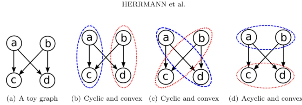
convex. On the other hand, convexity does not imply acyclicity. Figure 2.1 shows 117
that the definitions of an acyclic partition and a convex partition are not equivalent. 118
For the toy graph inFigure 2.1(a), there are three possible balanced partitions shown 119
in Figure 2.1(b),Figure 2.1(c), andFigure 2.1(d). They are all convex, but only the 120
one inFigure 2.1(d)is acyclic. 121
Deciding on the existence of a k-way acyclic partition respecting an upper bound 122
on the part weights and an upper bound on the cost of cut edges is NP-complete [13]. 123
The formal problem treated in this paper is defined as follows. 124
Definition 2.2 (DAG partitioning problem). Given a DAG G = (V, E) an im-125
balance parameter ε, find an acyclic k-way partition P = {V1, . . . , Vk} of V such that 126
a
b
c
d
(a) A toy graph
a
b
c
d
(b) Cyclic and convex
a
b
c
d
(c) Cyclic and convex
a
b
c
d
(d) Acyclic and convex
Fig. 2.1: A toy graph (left), two cyclic and convex partitions (middle two), and an acyclic and convex partition (right).
the balance constraints 127 (2.1) w(Vi) ≤ (1 + ε) P v∈V wv k 128
are satisfied for 1 ≤ i ≤ k, and the edge cut is minimized. 129
3. Related work. Fauzia et al. [11] propose a heuristic for the acyclic partition-130
ing problem to optimize data locality when analyzing DAGs. To create partitions, 131
the heuristic categorizes a vertex as ready to be assigned to a partition when all of 132
the vertices it depends on have already been assigned. Vertices are assigned to the 133
current partition set until the maximum number of vertices that would be “active” 134
during the computation of the part reaches a specified limit, which is the cache size 135
in their application. This implies that part sizes are not limited by the sum of the 136
total vertex weights but is a complex function that depends on an external schedule 137
(order) of the vertices. This differs from our problem as we limit the size of each part 138
by the total sum of the weights of the vertices on that part. 139
Kernighan [17] proposes an algorithm to find a minimum edge-cut partition of 140
the vertices of a graph into subsets of size greater than a lower bound and inferior 141
to an upper bound. The partition needs to use a fixed vertex sequence that cannot 142
be changed. Indeed, Kernighan’s algorithm takes a topological order of the vertices 143
of the graph as an input and partitions the vertices such that all vertices in a subset 144
constitute a continuous block in the given topological order. This procedure is optimal 145
for a given, fixed topological order and has a run time proportional to the number 146
of edges in the graph, if the part weights are taken as constant. We used a modified 147
version of this algorithm as a heuristic in the earlier version of our work [15]. 148
Cong et al. [7] describe two approaches for obtaining acyclic partitions of di-149
rected Boolean networks, modeling circuits. The first one is a single-level Fiduccia-150
Mattheyses (FM)-based approach. In this approach, Cong et al. generate an initial 151
acyclic partition by splitting the list of the vertices (in a topological order) from left 152
to right into k parts such that the weight of each part does not violate the bound. 153
The quality of the results is then improved with a k-way variant of the FM heuris-154
tic [12] taking the acyclicity constraint into account. Our previous work [15] employs 155
a similar refinement heuristic. The second approach of Cong et al. is a two-level 156
heuristic; the initial graph is first clustered with a special decomposition, and then it 157
is partitioned using the first heuristic. 158
In a recent paper [21], Moreira et al. focus on an imaging and computer vision 159
application on embedded systems and discuss acyclic partitioning heuristics. They 160
propose a single level approach in which an initial acyclic partitioning is obtained 161
using a topological order. To refine the partitioning, they proposed four local search 162
heuristics which respect the balance constraint and maintain the acyclicity of the 163
partition. Three heuristics pick a vertex and move it to an eligible part if and only if 164
the move improves the cut. These three heuristics differ in choosing the set of eligible 165
parts for each vertex; some are very restrictive, and some allow arbitrary target parts 166
as long as acyclicity is maintained. The fourth heuristic tentatively realizes the moves 167
that increase the cut in order to escape from a possible local minima. It has been 168
reported that this heuristic delivers better results than the others. In a follow-up 169
paper, Moreira et al. [22] discuss a multilevel graph partitioner and an evolutionary 170
algorithm based on this multilevel scheme. Their multilevel scheme starts with a 171
given acyclic partition. Then, the coarsening phase contracts edges that are in the 172
same part until there is no edge to contract. Here, matching-based heuristics from 173
undirected graph partitioning tools are used without taking the directions of the 174
edges into account. Therefore, the coarsening phase can create cycles in the graph; 175
however the induced partitions are never cyclic. Then, an initial partition is obtained, 176
which is refined during the uncoarsening phase with move-based heuristics. In order 177
to guarantee acyclic partitions, the vertices that lie in cycles are not moved. In a 178
systematic evaluation of the proposed methods, Moreira et al. note that there are 179
many local minima and suggest using relaxed constraints in the multilevel setting. 180
The proposed methods have high run time, as the evolutionary method of Moreira 181
et al. is not concerned with this issue. Improvements with respect to the earlier 182
work [21] are reported. 183
Previously, we had developed a multilevel partitioner [15]. In this paper, we 184
propose methods to use an undirected graph partitioner to guide the multilevel par-185
titioner. We focus on partitioning the graph in two parts since we can handle the 186
general case with a recursive bisection scheme. We also propose new coarsening, ini-187
tial partitioning, and refinement methods specifically designed for the 2-partitioning 188
problem. Our multilevel scheme maintains acyclic partitions and graphs through all 189
the levels. 190
Other related work on acyclic partitioning of directed graphs include an exact, 191
branch-and-bound algorithm by Nossack and Pesch [23] which works on the integer 192
programming formulation of the acyclic partitioning problem. This solution is, of 193
course, too costly to be used in practice. Wong et al. [29] present a modification of 194
the decomposition of Cong et al. [7] for clustering, and use this in a two-level scheme. 195
4. Directed multilevel graph partitioning. We propose a new multilevel tool 196
for obtaining acyclic partitions of directed acyclic graphs. Multilevel schemes [2,14] 197
form the de-facto standard for solving graph and hypergraph partitioning problems 198
efficiently, and used by almost all current state-of-the-art partitioning tools [3,14,16, 199
25,27]. Similar to other multilevel schemes, our tool has three phases: the coarsening 200
phase, which reduces the number of vertices by clustering them; the initial partitioning 201
phase, which finds a partition of the coarsest graph; and the uncoarsening phase, in 202
which the initial partition is projected to the finer graphs and refined along the way, 203
until a solution for the original graph is obtained. 204
4.1. Coarsening. In this phase, we obtain smaller DAGs by coalescing the ver-205
tices, level by level. This phase continues until the number of vertices becomes smaller 206
than a specified bound or the reduction on the number of vertices from one level to the 207
next one is lower than a threshold. At each level `, we start with a finer acyclic graph 208
G`, compute a valid clustering C`ensuring the acyclicity, and obtain a coarser acyclic 209
graph G`+1. While our previous work [15] discussed matching based algorithms for 210
coarsening, we present agglomerative clustering based variants here. The new vari-211
ants supersede the matching based ones. Unlike the standard undirected graph case, 212
in DAG partitioning, not all vertices can be safely combined. Consider a DAG with 213
three vertices a, b, c and three edges (a, b), (b, c), (a, c). Here, the vertices a and c 214
cannot be combined, since that would create a cycle. We say that a set of vertices is 215
contractible (all its vertices are matchable), if unifying them does not create a cycle. 216
We now present a general theory about finding clusters without forming cycles, after 217
giving some definitions. 218
Definition 4.1 (Clustering). A clustering of a DAG is a set of disjoint subsets 219
of vertices. Note that we do not make any assumptions on whether the subsets are 220
connected or not. 221
Definition 4.2 (Coarse graph). Given a DAG G and a clustering C of G, we 222
let G|C denote the coarse graph created by contracting all sets of vertices of C. 223
The vertices of the coarse graph are the clusters in C. If (u, v) ∈ G for two 224
vertices u and v that are located in different clusters of C then G|C has an (directed) 225
edge from the vertex corresponding to u’s cluster, to the vertex corresponding to v’s 226
cluster. 227
Definition 4.3 (Feasible clustering). A feasible clustering C of a DAG G is 228
a clustering such that G|C is acyclic. 229
Theorem 4.1. Let G = (V, E) be a DAG. For u, v ∈ V and (u, v) ∈ E, the coarse 230
graph G|{(u,v)} is acyclic if and only if there is no path from u to v in G avoiding the 231
edge (u, v). 232
Proof. Let G0 = (V0, E0) = G
|{(u,v)} be the coarse graph, and w be the merged, 233
coarser vertex of G0 corresponding to {u, v}. 234
If there is a path from u to v in G avoiding the edge (u, v), then all the edges of 235
this path are also in G0, and the corresponding path in G0goes from w to w, creating 236
a cycle. 237
Assume that there is a cycle in the coarse graph G0. This cycle has to pass through 238
w; otherwise, it must be in G which is impossible by the definition of G. Thus, there 239
is a cycle from w to w in the coarse graph G0. Let a ∈ V0 be the first vertex visited 240
by this cycle after w and b ∈ V0 be the last one, just before completing the cycle. Let 241
p be an a; b path in G0 such that (w, a) · p · (b, w) is the said w; w cycle in G0. 242
Note that a can be equal to b and in this case p = ∅. By the definition of the coarse 243
graph G0, a, b ∈ V and all edges in the path p are in E\{(u, v)}. Since we have a 244
cycle in G0, the following two items must hold: 245
• (i) either (u, a) ∈ E or (v, a) ∈ E, or both; and 246
• (ii) either (b, u) ∈ E or (b, v) ∈ E, or both. 247
Hence, overall we have nine (3×3) cases. Here, we investigate only four of them, as the 248
“both” conditions in (i) and (ii) can be eliminated easily by the following statements. 249
• (u, a) ∈ E and (b, u) ∈ E is impossible because otherwise, (u, a) · p · (b, u) 250
would be a u; u cycle in the original graph G. 251
• (v, a) ∈ E and (b, v) ∈ E is impossible because otherwise, (v, a) · p · (b, v) 252
would be a v; v cycle in the original graph G. 253
• (v, a) ∈ E and (b, u) ∈ E is impossible because otherwise, (u, v)·(v, a)·p·(b, u) 254
would be a u; u cycle in the original graph G. 255
Thus (u, a) ∈ E and (b, v) ∈ E. Therefore, (u, a) · p · (b, v) is a u; v path in G 256
avoiding the edge (u, v), which concludes the proof. 257
Theorem 4.1 can be extended to a set of vertices by noting that this time all 258
paths connecting two vertices of the set should contain only the vertices of the set. 259
The theorem (nor its extension) does not imply an efficient algorithm, as it requires 260
at least one transitive reduction. Furthermore, it does not describe a condition about 261
two clusters forming a cycle, even if both are individually contractible. In order to 262
address both of these issues, we put a constraint on the vertices that can form a 263
cluster, based on the following definition. 264
Definition 4.4 (Top level value). For a DAG G = (V, E), the top level value 265
of a vertex u ∈ V is the length of the longest path from a source of G to that vertex. 266
The top level values of all vertices can be computed in a single traversal of the graph 267
with a complexity O(|V | + |E|). We use top[u] to denote the top level of the vertex u. 268
The top level value of a vertex is independent of the topological order used for 269
computation. By restricting the set of edges considered in the clustering to the edges 270
(u, v) ∈ E such that top[u] + 1 = top[v], we ensure that no cycles are formed by 271
contracting a unique cluster (the condition identified inTheorem 4.1is satisfied). Let 272
C be a clustering of the vertices. Every edge in a cluster of C being contractible is a 273
necessary condition for C to be feasible, but not a sufficient one. More restrictions on 274
the edges of vertices inside the clusters should be found to ensure that C is feasible. 275
We propose three coarsening heuristics based on clustering sets of more than two 276
vertices, whose pair-wise top level differences are always zero or one. 277
4.1.1. Acyclic clustering with forbidden edges. To have an efficient heuris-278
tic, we rely only on static information computable in linear time while searching for 279
a feasible clustering. As stated in the introduction of this section, we rely on the 280
top level difference of one (or less) for all vertices in the same cluster, and an addi-281
tional condition to ensure that there will be no cycles when a number of clusters are 282
contracted simultaneously. In Theorem 4.2, we give two sufficient conditions for a 283
clustering to be feasible (that is, the graphs at all levels are DAGs) and prove their 284
correctness. 285
Theorem 4.2 (Correctness of the proposed clustering). Let G = (V, E) be a 286
DAG and C = {C1, . . . , Ck} be a clustering. If C is such that: 287
• for any cluster Ci, for all u, v ∈ Ci, |top[u] − top[v]| ≤ 1, 288
• for two different clusters Ci and Cj and for all u ∈ Ci and v ∈ Cj either 289
(u, v) /∈ E, or top[u] 6= top[v] − 1, 290
then, the coarse graph G|C is acyclic. 291
Proof. Let us assume (for the sake of contradiction) that there is a clustering 292
with the same properties above, but the coarsened graph has a cycle. We pick one 293
such clustering C = {C1, . . . , Ck} with the minimum number of clusters. Let ti = 294
min{top[u], u ∈ Ci} be the smallest top level value of a vertex of Ci. According to the 295
properties of C, for every vertex u ∈ Ci, either top[u] = ti, or top[u] = ti+ 1. Let wi 296
be the coarse vertex in G|C obtained by contracting all vertices in Ci, for i = 1, . . . , k. 297
By the assumption, there is a cycle in G|C, and let c be one with the minimum length. 298
This cycle passes through all the wi vertices. Otherwise, there would be a smaller 299
cardinality clustering with the properties above and creating a cycle in the coarsened 300
graph, contradicting the minimal cardinality of C. Let us renumber, without loss of 301
generality, the wi vertices such that c is a w1 ; w1 cycle which passes through all 302
the wi vertices in the non-decreasing order of the indices. This also renumbers the 303
clusters accordingly. 304
After renumbering the wivertices, for every i ∈ {1, . . . , k}, there is a path in G|C 305
from wito wi+1. Given the definition of the coarsened graph, for every i ∈ {1, . . . , k} 306
there exists a vertex ui ∈ Ci, and a vertex ui+1 ∈ Ci+1 such that there exists a 307
path ui ; ui+1 in G. Thus, top[ui] + 1 ≤ top[ui+1]. According to the second 308
property, either there is at least one intermediate vertex between ui and ui+1 and 309
then top[ui] + 1 < top[ui+1]; or top[ui] + 1 6= top[ui+1] and then top[ui] + 1 < 310
top[ui+1]. Thus, in any case, top[ui] + 1 < top[ui+1] which can be rewritten as 311
top[ui] < top[ui+1] − 1. 312
By definition, we know that ti≤ top[ui] and top[ui+1] − 1 ≤ ti+1. Thus for every 313
i ∈ {1, . . . , k}, we have ti < ti+1, which leads to the self-contradicting statement 314
t1< tk+1= t1 and concludes the proof. 315
The main heuristic based on Theorem 4.2 is described in Algorithm 1. This 316
heuristic visits all vertices in an order, and adds the visited vertex to a cluster, if 317
certain criteria are met; if not, the vertex stays as a singleton. When visiting a 318
singleton vertex, the clusters of its in-neighbors and out-neighbors are investigated, 319
and the best (according to an objective value) among those meeting the criterion 320
described inTheorem 4.2is selected. 321
Algorithm 1 returns the leader array of each vertex for the current coarsening 322
step. Vertices with the same leader form a cluster (and will form a single vertex in 323
the coarsened graph). For each vertex u ∈ V , leader[u] is the id of the representative 324
vertex for the cluster that will contain u after Algorithm 1. The leader table will 325
be used to build the coarse graph. Any arbitrary vertex in a given cluster can be 326
used as the leader of this cluster without impacting the rest of the algorithm. At the 327
beginning, each vertex belongs to a singleton cluster, and leader[u] = u. To keep 328
the track of trivial clusters (singleton vertices), we use an auxiliary mark array. The 329
value mark[u] is false if u still belongs to a singleton cluster. Otherwise, the value is 330
set to true. 331
For each singleton vertex u, we maintain an auxiliary array nbbadneighbors to 332
keep the number of non-trivial bad neighbor clusters. That is to say, the number 333
of clusters containing a neighbor of u that would violate the second condition of 334
Theorem 4.2 in case u was put in another cluster. Hence, if u has only one bad 335
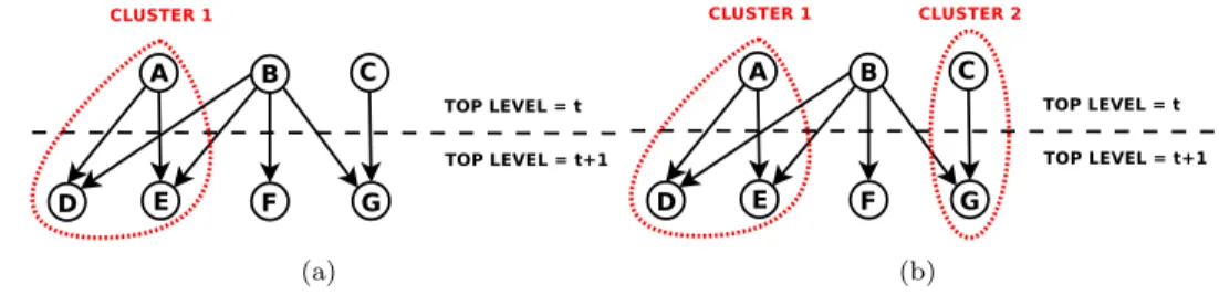
neighbor cluster, it can only be put into this cluster. For instance in Figure 4.1(a), 336
at this point of the coarsening, vertex B can only be put in Cluster 1. Otherwise, if 337
vertex B was matched with one of its other neighbors, the second condition of the 338
theorem would be violated. Thus, if a vertex has more than one bad neighbor in 339
different clusters, it has to stay as a singleton. For instance in Figure 4.1(b), vertex 340
B has two bad neighbor clusters and cannot be put in any cluster without violating 341
the second condition of Theorem4.2. To check if there exists another bad neighbor 342
cluster previously formed, we maintain an array leaderbadneighbor that keeps the 343
representative/leader of the first bad neighbor cluster for each vertex. Initially, this 344
value is set to minus one. 345
In Algorithm 1, the function ValidNeighbors selects the compatible neighbors of 346
vertex u, that is the neighbors in clusters that vertex u can join. This selection is 347
based on the top level difference (to respect the first condition of Theorem4.2), the 348
number of bad neighbors of u, and u’s neighbors (to respect the second condition of 349
Theorem 4.2), and the size limitation (we do not want a cluster to be bigger than 350
10% of the total weight of the graph). Then, a best neighbor, BestN eigh, according 351
to an objective value, such as the edge cost, is selected. After setting the leader of 352
vertex u to the same value as the leader of BestN eigh, some bookkeeping is done 353
for the arrays related to the second condition of Theorem 4.2. More precisely, at 354
Lines 16–22 of Algorithm1, the neighbors of u are informed about u joining a new 355
cluster, potentially becoming a bad neighbor. While doing that, the algorithm skips 356
the vertices v such that |top[u] − top[v]| > 1, since u cannot form a bad neighbor 357
cluster for such v. Similarly, if the best neighbor chosen for u was not in a cluster 358
previously, i.e., was a singleton vertex, the number of bad neighbors of its neighbors 359
are updated (Lines24–30). 360
(a) (b)
Fig. 4.1: Two examples of acyclic clustering.
In our framework, we also implemented the version in the preliminary study [15] 361
where the size of cluster is limited to two, meaning that it computes a matching of 362
the vertices. 363
It can be easily seen that Algorithm1has a worst case time complexity of O(|V |+ 364
|E|). The array top is constructed in O(|V | + |E|) time, and the best, valid neighbor 365
of a vertex u is found in O(|Neigh[u]|) time. The neighbors of a vertex are visited at 366
most once to keep the arrays related to the second condition of Theorem 4.2 up to 367
date at Lines16and24. 368
4.1.2. Acyclic clustering with cycle detection. We now propose a less re-369
strictive clustering algorithm to ensure that the acyclicity of the coarse graph is 370
maintained. As in the previous section, we rely on the top level difference of one 371
(or less) for all vertices in the same cluster, i.e., for any cluster Ci, for all u, v ∈ Ci, 372
|top[u]−top[v]| ≤ 1. Knowing this invariant, when a new vertex is added to a cluster, 373
a cycle-detection algorithm checks that no cycles are formed when all the clusters are 374
contracted simultaneously. This algorithm does not traverse the entire graph by also 375
using the fact that the top level difference within a cluster is at most one. 376
From the proof ofTheorem 4.2, we know that with a feasible clustering, if adding 377
a vertex to a cluster whose vertices’ top level values are t and t + 1 creates a cycle 378
in the contracted graph, then this cycle goes through only the vertices with top level 379
values t or t + 1. Thus, when considering the addition of a vertex u to a cluster C 380
containing v, we check potential cycle formations by traversing the graph starting 381
from u in a breadth-first manner in the DetectCycle function used in Algorithm 2. 382
Let t denote the minimum top level in C. When at a vertex w, we normally add a 383
successor y of w into the queue, if |top(y) − t| ≤ 1; if w is in the same cluster as one 384
of its predecessors x, we also add x to the queue if |top(x) − t| ≤ 1. This function 385
uses markers to not to visit the same vertex multiple times, returns true if at some 386
point in the traversal a vertex from cluster C is reached, and returns false, otherwise. 387
In the worst-case, this cycle detection algorithm completes a full graph traversal but 388
in practice, it stops quickly and does not introduce a significant overhead. 389
Here, we propose different clustering strategies. These algorithms consider all 390
the vertices in the graph, one by one, and put them in a cluster if their top level 391
Algorithm 1: Clustering with forbidden edges
Data: Directed graph G = (V, E), a traversal order of the vertices in V , a priority on edges
Result: The leader array for the coarsening
1 top ← CompTopLevels(G)
/* Initialize all the auxiliary data to be used */
2 for u ∈ V do
3 mark[u] ← f alse // all vertices are marked as singleton
4 leader[u] ← u
5 weight[u] ← wu // keeps the total weight for each cluster /* nbbadneighbors[u] stores the number of bad clusters for a vertex u. If
it exceeds one, u is left alone (the second condition of Theorem 4.2.). */
6 nbbadneighbors[u] ← 0
7 leaderbadneighbors[u] ← −1
8 for u ∈ V following the traversal order in input do 9 if mark[u] then continue
/* The function ValidNeighbors returns the set of valid match candidates for u based on Theorem 4.2. It also checks the threshold for the maximum cluster size, and the number of bad neighbor clusters for u. */
10 N ← ValidNeighbors(u, G, nbbadneighbors, leaderbadneighbors, weight) 11 if N = ∅ then continue
12 BestN eigh ← BestNeighbour(N ) 13 ` ← leader[BestN eigh]
14 leader[u] ← ` // assign u to BestNeigh’s cluster
15 weight[`] ← weight[`] + wu
/* Let the neighbors of u know that it is not a singleton anymore */
16 for v ∈ Neigh[u] do
17 if |top[u] − top[v]| > 1 then continue // u cannot form a bad cluster
18 if nbbadneighbors[v] = 0 then 19 nbbadneighbors[v] ← 1
20 leaderbadneighbors[v] ← `
21 else if nbbadneighbors[v] = 1 and leaderbadneighbors[v] 6= ` then
22 nbbadneighbors[v] ← 2 // mark v as unmatchable
/* If BestNeigh was forming a singleton cluster before u’s assignment */
23 if mark[BestN eigh] = f alse then
/* Let BestNeigh’s neighbors know that it is not a singleton anymore */
24 for v ∈ Neigh[BestN eigh] do
25 if |top[BestN eigh] − top[v]| > 1 then continue 26 if nbbadneighbors[v] = 0 then
27 nbbadneighbors[v] ← 1 // The first bad neighbor cluster for v
28 leaderbadneighbors[v] ← `
29 else if nbbadneighbors[v] = 1 and leaderbadneighbors[v] 6= ` then
30 nbbadneighbors[v] ← 2 // mark v as unmatchable
31 mark[BestN eigh] ← true // BestNeigh is not a singleton anymore
32 mark[u] ← true // u is not a singleton anymore
33 return leader
differences are at most one and if no cycles are introduced. The clustering algorithms 392
depending on different vertex traversal orders and priority definitions on the adjacent 393
edges are described in Algorithm2. As Algorithm 1, this algorithm also returns the 394
leader array of each vertex for the current coarsening step. When a vertex is put in a 395
cluster with top level values t and t + 1, its markup (respectively markdown) value is 396
set to true if its top level value is t (respectively t+1). Since the worst case complexity 397
of the cycle detection is O(|V | + |E|), the worst case complexity of Algorithm 2 is 398
O(|V |(|V | + |E|)). However, the cycle detection stops quickly in practice and the 399
behavior of Algorithm2is closer to O(|V | + |E|) as described inSubsection 5.6. 400
Algorithm 2: Clustering with cycle detection
Data: Directed graph G = (V, E), a traversal order of the vertices in V , a priority on edges
Result: A feasible clustering C of G 1 top ← CompTopLevels(G)
2 for u ∈ V do
3 markup[u] ← f alse // if u’s cluster has a v with top[v] = top[u] + 1 4 markdown[u] ← f alse // if u’s cluster has a v with top[v] = top[u] − 1 5 leader[u] ← u // the leader vertex id for u’s cluster 6 for u ∈ V following the traversal order in input do
7 if markup[u] or markdown[u] then continue
8 for v ∈ Neigh[u] following given priority on edges do
9 if (|top[u] − top[v]| > 1) then continue // we use |top[u] − top[v]| = 1
/* If this is a (u, v) edge */
10 if v ∈ Succ[u] then
11 if markup[v] then continue
12 if DetectCycle(u, v, G, leader) then continue 13 leader[u] ← leader[v]
14 markup[u] ← markdown[v] ← true
/* If this is a (v, u) edge */
15 if v ∈ Pred[u] then
16 if markdown[v] then continue
17 if DetectCycle(u, v, G, leader) then continue 18 leader[u] ← leader[v]
19 markdown[u] ← markup[v] ← true
20 return leader
4.1.3. Hybrid acyclic clustering. The cycle detection based algorithm can 401
suffer from quadratic run time for vertices with large in-degrees or out-degrees. To 402
avoid this, we design a hybrid acyclic clustering which uses the clustering strategy 403
described in Algorithm 2 by default and switches to the clustering strategy in Al-404
gorithm 1 for large degree vertices. We define a limit on the degree of a vertex 405
(typicallyp|V |/10) for calling it large degree. When considering an edge (u, v) where 406
top[u] + 1 = top[v], if the degrees of u and v do not exceed the limit, we use the cycle 407
detection algorithm to determine if we can contract the edge. Otherwise, if the out-408
degree of u or the indegree of v is too large, the edge will be contracted if Algorithm1
409
allows so. The complexity of this algorithm is in between those of Algorithm1 and 410
Algorithm2and will likely avoid the quadratic behavior in practice (if not, the degree 411
parameter can be adapted). 412
4.2. Initial partitioning. After the coarsening phase, we compute an initial 413
acyclic partitioning of the coarsest graph. We present two heuristics. One of them 414
is akin to the greedy graph growing method used in the standard graph/hypergraph 415
partitioning methods. The second one uses an undirected partitioning and then fixes 416
the acyclicity of the partitions. Throughout this section, we use (V0, V1) to denote 417
the bisection of the vertices of the coarsest graph G. The acyclic bisection (V0, V1) is 418
such that there is no edge from the vertices in V1 to those in V0. 419
4.2.1. Greedy directed graph growing. One approach to compute a bisec-420
tion of a directed graph is to design a greedy algorithm that moves vertices from one 421
part to another using local information. Greedy algorithms have shown to be effective 422
for initial partitioning in multilevel schemes in the undirected case. We start with 423
all vertices in V1 and replace vertices towards V0 by using heaps. At any time, the 424
vertices that can be moved to V0 are in the heap. These vertices are those whose all 425
in-neighbors are in V0. Initially only the sources are in the heap, and when all the 426
in-neighbors of a vertex v are moved to the first part, v is inserted into the heap. We 427
separate this process into two phases. In the first phase, the key-values of the vertices 428
in the heap are set to the weighted sum of their incoming edges, and the ties are bro-429
ken in favor of the vertex closer to the first vertex moved. The first phase continues 430
until the first part has more than 0.9 of the maximum allowed weight (modulo the 431
maximum weight of a vertex). In the second phase, the actual gain of a vertex is 432
used. This gain is equal to the sum of the weights of the incoming edges minus the 433
sum of the weights of the outgoing edges. In this phase, the ties are broken in favor 434
of the heavier vertices. The second phase stops as soon as the required balance is 435
obtained. The reason that we separated this heuristic into two phases is that at the 436
beginning, the gains are of no importance, and the more vertices become movable the 437
more flexibility the heuristic has. Yet, towards the end, parts are fairly balanced, and 438
using actual gains can help keeping the cut small. 439
Since the order of the parts is important, we also reverse the roles of the parts, 440
and the directions of the edges. That is, we put all vertices in V0, and move the 441
vertices one by one to V1, when all out-neighbors of a vertex have been moved to V1. 442
The proposed greedy directed graph growing heuristic returns the best of the these 443
two alternatives. 444
4.2.2. Undirected bisection and fixing acyclicity. In this heuristic, we par-445
tition the coarsest graph as if it were undirected and then move the vertices from one 446
part to another in case the partition was not acyclic. Let (P0, P1) denote the (not 447
necessarily acyclic) bisection of the coarsest graph treated as if it were undirected. 448
The proposed approach designates arbitrarily P0as V0and P1as V1. One way to 449
fix the cycle is to move all ancestors of the vertices in V0 to V0, thereby guaranteeing 450
that there is no edge from vertices in V1to vertices in V0, making the bisection (V0, V1) 451
acyclic. We do these moves in a reverse topological order, as shown in Algorithm3. 452
Another way to fix the acyclicity is to move all descendants of the vertices in V1 453
to V1, again guaranteeing an acyclic partition. We do these moves in a topological 454
order, as shown in Algorithm4. We then fix the possible unbalance with a refinement 455
algorithm. 456
Note that we can also initially designate P1 as V0 and P0 as V1, and again use 457
Algorithms3 and 4 to fix a potential cycle in two different ways. We try all four of 458
these choices, and return the best partition (essentially returning the best of the four 459
choices to fix the acyclicity of (P0, P1)). 460
4.3. Refinement. This phase projects the partition obtained for a coarse graph 461
to the next, finer one and refines the partition by vertex moves. As in the standard 462
refinement methods, the proposed heuristic is applied in a number of passes. Within a 463
pass, we repeatedly select the vertex with the maximum move gain among those that 464
can be moved. We tentatively realize this move if the move maintains or improves 465
the balance. Then, the most profitable prefix of vertex moves are realized at the end 466
of the pass. As usual, we allow the vertices move only once in a pass; therefore once a 467
vertex is moved, it is not eligible to move again during the same pass. We use heaps 468
Algorithm 3: fixAcyclicityUp
Data: Directed graph G = (V, E) and a bisection part Result: An acyclic bisection of G
1 for u ∈ G (in reverse topological order) do 2 if part[u] = 0 then
3 for v ∈ Pred[u] do 4 part[v] ← 0
5 return part
Algorithm 4: fixAcyclicityDown
Data: Directed graph G = (V, E) and a bisection part Result: An acyclic bisection of G
1 for u ∈ G (in topological order) do 2 if part[u] = 1 then
3 for v ∈ Succ[u] do 4 part[v] ← 1
5 return part
with the gain of moves as the key value, where we keep only movable vertices. We 469
call a vertex movable, if moving it to the other part does not create a cyclic partition. 470
As previously done, we use the notation (V0, V1) to designate the acyclic bisection 471
with no edge from vertices in V1 to vertices in V0. This means that for a vertex to 472
move from part V0to part V1, one of the two conditions should be met (i) either all its 473
out-neighbors should be in V1; (ii) or the vertex has no out-neighbors at all. Similarly, 474
for a vertex to move from part V1to part V0, one of the two conditions should be met 475
(i) either all its in-neighbors should be in V0; (ii) or the vertex has no in-neighbors 476
at all. This is in a sense the adaptation of boundary Fiduccia-Mattheyses [12] (FM) 477
to directed graphs, where the boundary corresponds to the movable vertices. The 478
notion of movability being more restrictive results in an important simplification with 479
respect to the undirected case. The gain of moving a vertex v from V0to V1 is 480 (4.1) X u∈Succ[v] w(v, u) − X u∈Pred[v] w(u, v) , 481
and the negative of this value when moving it from V1to V0. This means that the gain 482
of vertices are static: once a vertex is inserted in the heap with the key value (4.1), 483
it is never updated. A move could render some vertices unmovable; if they were in 484
the heap, then they should be deleted. Therefore, the heap data structure needs to 485
support insert, delete, and extract max operations only. 486
We have also implemented a swapping based refinement heuristic akin to the 487
boundary Kernighan-Lin [18] (KL), and another one moving vertices only from the 488
maximum loaded part. For graphs with unit weight vertices, we suggest using the 489
boundary FM, and for others we suggest using one pass of boundary KL followed by 490
one pass of the boundary FM that moves vertices only from the maximum loaded 491
part. 492
4.4. Constraint coarsening and initial partitioning. There are a number 493
of highly successful, undirected graph partitioning libraries [16, 25, 27]. They are 494
8 1 58 64 32 33 27 45 48 41 35 53 38 15 22
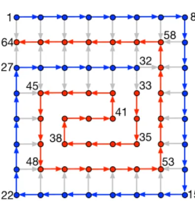
Fig. 4.2: 8 × 8 grid graph whose vertices are ordered in a spiral way; a few of the vertices are labeled with their number. All edges are oriented from a lower numbered vertex to a higher numbered one. There is a unique bipartition with 32 vertices in each side. The edges defining the total order are shown in red and blue, except the one from 32 to 33; the cut edges are shown in gray; other internal edges are not shown.
not directly usable for our purposes, as the partitions can be cyclic. Fixing such 495
partitions, by moving vertices to break the cyclic dependencies among the parts, can 496
increase the edge cut dramatically (with respect to the undirected cut). Consider for 497
example, the n × n grid graph, where the vertices are integer positions for i = 1, . . . n 498
and j = 1, . . . , n and a vertex at (i, j) is connected to (i0, j0) when |i − i0| = 1 or 499
|j − j0| = 1, but not both. There is an acyclic orientation of this graph, called spiral 500
ordering, as described in Figure 4.2 for n = 8. This spiral ordering defines a total 501
order. When the directions of the edges are ignored, we can have a bisection with 502
perfect balance by cutting only n = 8 edges with a vertical line. This partition is 503
cyclic; and it can be made acyclic by putting all vertices numbered greater than 32 504
to the second part. This partition, which puts the vertices 1–32 to the first part and 505
the rest to the second part, is the unique acyclic bisection with perfect balance for 506
the associated directed acyclic graph. The edge cut in the directed version is 35 as 507
seen in the figure (gray edges). In general one has to cut n2− 4n + 3 edges for n ≥ 8: 508
the blue vertices in the border (excluding the corners) have one edge directed to a red 509
vertex; the interior blue vertices have two such edges; finally, the blue vertex labeled 510
n2/2 has three such edges. 511
Let us also investigate the quality of the partitions from a more practical stand-512
point. We used MeTiS [16] as the undirected graph partitioner on a dataset of 94 513
matrices (their details are in Section 5). The results are given in Figure 4.3. For 514
this preliminary experiment, we partitioned the graphs into two with the maximum 515
allowed load imbalance ε = 3%. In the experiment, for only two graphs, the output 516
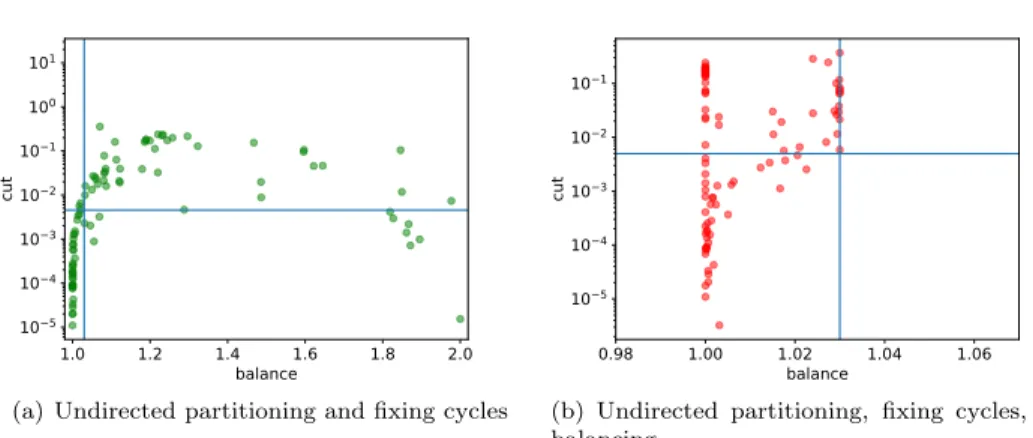
of MeTiS is acyclic, and the geometric mean of the normalized edge cut is 0.0012. 517
Figure 4.3(a)shows the normalized edge cut and the load imbalance after fixing the 518
cycles, while Figure 4.3(b) shows the two measurements after meeting the balance 519
criteria. A normalized edge cut value is computed by normalizing the edge cut with 520
respect to the number of edges. 521
In both figures, the horizontal lines mark the geometric mean of the normalized 522
edge cuts, and the vertical lines mark the 3% imbalance ratio. InFigure 4.3(a), there 523
are 37 instances in which the load balance after fixing the cycles is feasible. The 524
1.0 1.2 1.4 1.6 1.8 2.0 balance 105 104 103 102 101 100 101 cut
(a) Undirected partitioning and fixing cycles
0.98 1.00 1.02 1.04 1.06 balance 105 104 103 102 101 cut
(b) Undirected partitioning, fixing cycles, and balancing
Fig. 4.3: Normalized edge cut (normalized with respect to the number of edges), and the balance obtained after using an undirected graph partitioner and fixing the cycles (left), and after ensuring balance with refinement (right).
geometric mean of the normalized edge cuts in this subfigure is 0.0045, while in the 525
other subfigure, it is 0.0049. Fixing the cycles increases the edge cut with respect to 526
an undirected partitioning, but not catastrophically (only by 0.0045/0.0012 = 3.75 527
times in these experiments), and achieving balance after this step increases the cut 528
only a little (goes to 0.0049 from 0.0045). That is why we suggest using an undirected 529
graph partitioner, fixing the cycles among the parts, and performing a refinement 530
based method for load balancing as a good (initial) partitioner. 531
In order to refine the initial partition in a multilevel setting, we propose a scheme 532
similar to the iterated multilevel algorithm used in the existing partitioners [3,28]. In 533
this scheme, first a partition P is obtained. Then, the coarsening phase is employed 534
to match (or to agglomerate) the vertices that were in the same part in P . After 535
the coarsening, an initial partitioning is freely available by using the partition P 536
on the coarsest graph. The refinement phase then can work as before. Moreira 537
et al. [22] use this approach for the directed graph partitioning problem. To be 538
more concrete, we first use an undirected graph partitioner, then fix the cycles as 539
discussed inSection 4.2.2, and then refine this acyclic partition for balance with the 540
proposed refinement heuristics inSubsection 4.3. We then use this acyclic partition for 541
constraint coarsening and initial partitioning. We expect this scheme to be successful 542
in graphs with many sources and targets where the sources and targets can lie in any 543
of the parts while the overall partition is acyclic. On the other hand, if a graph is such 544
that its balanced acyclic partitions need to put sources in one part and the targets in 545
another part, then fixing acyclicity may result in moving many vertices. This in turn 546
will harm the edge cut found by the undirected graph partitioner. 547
5. Experimental evaluation. The partitioning tool presented (dagP) is imple-548
mented in C/C++ programming languages. The experiments are conducted on a 549
computer equipped with dual 2.1 GHz, Xeon E5-2683 processors and 512GB memory. 550
The source code and more information is available athttp://tda.gatech.edu/software/ 551
dagP/.
552
We have performed an extensive evaluation of the proposed multilevel directed 553
Graph Parameters #vertex #edge max. deg. avg. deg. #source #target 2mm P=10, Q=20, R=30, 36,500 62,200 40 1.704 2100 400 S=40 3mm P=10, Q=20, R=30, 111,900 214,600 40 1.918 3900 400 S=40, T=50 adi T=20, N=30 596,695 1,059,590 109,760 1.776 843 28 atax M=210, N=230 241,730 385,960 230 1.597 48530 230 covariance M=50, N=70 191,600 368,775 70 1.925 4775 1275 doitgen P=10, Q=15, R=20 123,400 237,000 150 1.921 3400 3000 durbin N=250 126,246 250,993 252 1.988 250 249 fdtd-2d T=20, X=30, Y=40 256,479 436,580 60 1.702 3579 1199 gemm P=60, Q=70, R=80 1,026,800 1,684,200 70 1.640 14600 4200 gemver N=120 159,480 259,440 120 1.627 15360 120 gesummv N=250 376,000 500,500 500 1.331 125250 250 heat-3d T=40, N=20 308,480 491,520 20 1.593 1280 512 jacobi-1d T=100, N=400 239,202 398,000 100 1.664 402 398 jacobi-2d T=20, N=30 157,808 282,240 20 1.789 1008 784 lu N=80 344,520 676,240 79 1.963 6400 1 ludcmp N=80 357,320 701,680 80 1.964 6480 1 mvt N=200 200,800 320,000 200 1.594 40800 400 seidel-2d M=20, N=40 261,520 490,960 60 1.877 1600 1 symm M=40, N=60 254,020 440,400 120 1.734 5680 2400 syr2k M=20, N=30 111,000 180,900 60 1.630 2100 900 syrk M=60, N=80 594,480 975,240 81 1.640 8040 3240 trisolv N=400 240,600 320,000 399 1.330 80600 1 trmm M=60, N=80 294,570 571,200 80 1.939 6570 4800
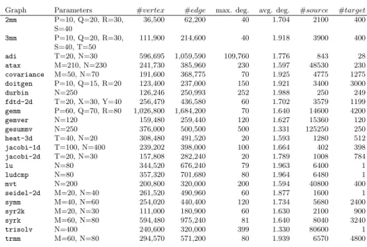
Table 5.1: Instances from the Polyhedral Benchmark suite (PolyBench).
acyclic graph partitioning method on DAG instances coming from two sources. The 554
first set of instances is from the Polyhedral Benchmark suite (PolyBench) [26], whose 555
parameters are listed in Table 5.1. The graphs in the Polyhedral Benchmark suite 556
arise from various linear computation kernels. The parameters in the second column 557
ofTable 5.1represent the size of these computation kernels. For more details, we re-558
fer the reader to the description of the Polyhedral Benchmark suite (PolyBench) [26]. 559
The second set of instances is obtained from the matrices available in the SuiteS-560
parse Matrix Collection (formerly known as the University of Florida Sparse Matrix 561
Collection) [8]. From this collection, we pick all the matrices satisfying the following 562
properties: listed as binary, square, and has at least 100000 rows and at most 226 563
nonzeros. There were a total of 95 matrices at the time of experimentation, where 564
two matrices (ids 1514 and 2294) having the same pattern. We discard the duplicate 565
and use the remaining 94 matrices for experiments. For each such matrix, we take 566
the strict upper triangular part as the associated DAG instance, whenever this part 567
has more nonzeros than the lower triangular part; otherwise we take the strict lower 568
triangular part. All edges have unit cost, and all vertices have unit weight. 569
Since the proposed heuristics have a randomized behavior (the traversals used 570
in the coarsening and refinement heuristics are randomized), we run them 10 times 571
for each DAG instance, and report the averages of these runs. We use performance 572
profiles [9] to present the edge-cut results. A performance profile plot shows the 573
probability that a specific method gives results within a factor θ of the best edge cut 574
obtained by any of the methods compared in the plot. Hence, the higher and closer 575
a plot to the y-axis, the better the method is. 576
We set the load imbalance parameter ε = 0.03 in (2.1) for all experiments. The 577
vertices are unit weighted, therefore, the imbalance is rarely an issue for a move-based 578
partitioner. 579
1.0 1.2 1.4 1.6 1.8 0.0 0.2 0.4 0.6 0.8 1.0
p
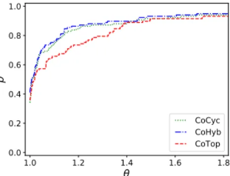
CoCyc CoHyb CoTopFig. 5.1: Performance profiles of the proposed multilevel algorithm variants using three difference coarsening heuristics in terms of edge cut.
5.1. Coarsening evaluation. We first evaluate the proposed coarsening heuris-580
tics. The aim is to find an effective one to set as a default coarsening heuristic. 581
The performance profile chart given inFigure 5.1shows the effect of the coarsen-582
ing heuristics on the final edge cut for the whole dataset. The variants of the proposed 583
multilevel algorithm which use different coarsening schemes are named as CoTop (
Sec-584
tion 4.1.1), CoCyc (Section 4.1.2), and CoHyb (Section 4.1.3). Here, and in the rest of 585
the paper, we used a randomized Depth-First topological order for the node traversal 586
in the coarsening heuristics, since it performed better in practice. In Figure 5.1, we 587
see that CoCyc and CoHyb behave similarly; this is expected as not all graphs have 588
vertices with large degrees. From this figure, we conclude that in general, the coars-589
ening heuristics CoHyb and CoCyc are more helpful than CoTop in reducing the edge 590
cut. 591
Another important characteristic to assess for a coarsening heuristic is its con-592
traction efficiency. It is important that the coarsening phase does not stop too early 593
and that the coarsest graph is small enough to be partitioned efficiently. Table 5.2
594
gives the maximum, the average, and the standard deviation of vertex and edge weight 595
ratios, and the average, the minimum, and the maximum number of coarsening levels 596
observed for the two datasets. An effective coarsening heuristic should have small 597
vertex and edge weight ratios. We see that CoCyc and CoHyb behave similarly and 598
provide slightly better results than CoTop on both datasets. The graphs from the two 599
datasets have different characteristics. All coarsening heuristics perform better on the 600
PolyBench instances compared to the UFL instances: they obtain smaller ratios in 601
the number of remaining vertices, and yield smaller edge weights. Furthermore, the 602
maximum vertex and edge weight ratios are smaller in PolyBench instances, again 603
with all coarsening methods. To the best of our understanding, these happen due to 604
two reasons; (i) the average degree in the UFL instances is larger than that of the 605
PolyBench instances (3.63 vs. 1.72); (ii) the ratio of the total number of source and 606
target vertices to the total number of vertices is again larger in the UFL instances 607
(0.13 vs. 0.03). Based on Figure 5.1 and Table 5.2, we set CoHyb as the default 608
coarsening heuristic, as it performs better than CoTop in terms of final edge cut, and 609
is guaranteed to be more efficient than CoCyc in terms of run time. 610
5.2. Constraint coarsening and initial partitioning. We now investigate 611
the effect of using undirected graph partitioners to obtain a more effective coarsen-612
Algorithm Vertex ratio (%) Edge weight ratio (%) Coarsening levels avg std. dev max avg std. dev max avg min max CoTop 1.29 6.34 46.72 26.07 24.95 87.00 12.45 2 17.0 CoCyc 1.06 6.31 47.29 25.97 24.86 87.90 12.74 2 17.6 CoHyb 1.08 6.27 46.70 26.00 24.80 87.00 12.69 2 17.7 CoTop 1.33 2.26 8.50 25.67 11.08 47.60 7.44 4 11.8 CoCyc 0.41 0.90 4.10 24.96 9.20 37.00 8.37 5 12.0 CoHyb 0.54 0.88 3.60 24.81 9.33 39.00 8.46 5 11.9 Table 5.2: The maximum, average, and standard deviation of vertex and edge weight ratios, and the average, the minimum, and the maximum number of coarsening levels for the UFL dataset on the upper half of the table, and for the PolyBench dataset on the lower half.
ing and better initial partitions as explained in Subsection 4.4. We compare three 613
variants of the proposed multilevel scheme. All of them use the refinement described 614
inSubsection 4.3in the uncoarsening phase. 615
• CoHyb: this variant uses the hybrid coarsening heuristic described in
Sec-616
tion 4.1.3and the greedy directed graph growing heuristic described in
Sec-617
tion 4.2.1 in the initial partitioning phase. This method does not use con-618
straint coarsening. 619
• CoHyb C: this variant uses an acyclic partition of the finest graph obtained as 620
outlined inSection 4.2.2 to guide the hybrid coarsening heuristic described 621
inSubsection 4.4, and uses the greedy directed graph growing heuristic in the 622
initial partitioning phase. 623
• CoHyb CIP: this variant uses the same constraint coarsening heuristic as the 624
previous method, but inherits the fixed acyclic partition of the finest graph 625
as the initial partitioning. 626
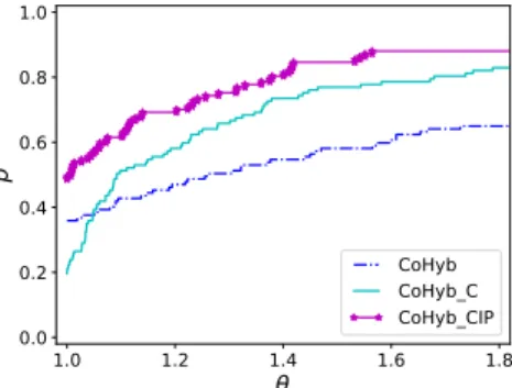
The comparison of these three variants are given in Figure 5.2 for the whole 627
dataset. FromFigure 5.2, we see that using the constraint coarsening is always helpful 628
with respect to not using them. This clearly separates CoHyb C and CoHyb CIP from 629
CoHyb after θ = 1.1. Furthermore, applying the constraint initial partitioning (on top 630
of the constraint coarsening) brings tangible improvements. 631
In the light of the experiments presented here, we suggest the variant CoHyb CIP 632
for general problem instances, as this has clear advantages over others in our dataset. 633
5.3. Evaluating CoHyb CIP with respect to a single level algorithm. We 634
compare CoHyb CIP (the variant of the proposed approach with constraint coarsening 635
and initial partitioning) with a single-level algorithm that uses an undirected graph 636
partitioning, fixes the acyclicity, and refines the partitions. This last variant is denoted 637
as UndirFix, and it is the algorithm described in Section 4.2.2. Both variants use 638
the same initial partitioning approach, which utilizes MeTiS [16] as the undirected 639
partitioner. The difference between UndirFix and CoHyb CIP is the latter’s ability to 640
refine the initial partition at multiple levels. Figure5.3presents this comparison. The 641
plots show that the multilevel scheme CoHyb CIP outperforms the single level scheme 642
UndirFix at all appropriate ranges of θ, attesting to the importance of the multilevel 643
scheme. 644
5.4. Comparison with existing work. Here we compare our approach with 645
the evolutionary graph partitioning approach developed by Moreira et al. [21], and 646
1.0 1.2 1.4 1.6 1.8 0.0 0.2 0.4 0.6 0.8 1.0
p
CoHyb CoHyb_C CoHyb_CIPFig. 5.2: Performance profiles for the edge cut obtained by the proposed multilevel algorithm using the constraint coarsening and partitioning (CoHyb CIP), using the constraint coarsening and the greedy directed graph growing (CoHyb C), and the best identified approach without constraints (CoHyb).
1.0 1.2 1.4 1.6 1.8 0.0 0.2 0.4 0.6 0.8 1.0
p
CoHyb_CIP UndirFixFig. 5.3: Performance profiles for the edge cut obtained by the proposed multilevel approach using the constraint coarsening and partitioning (CoHyb CIP) and using the same approach without coarsening (UndirFix).
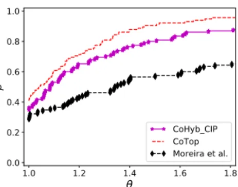
briefly with our previous work [15]. 647
Figure 5.4 shows how CoHyb CIP and CoTop compare with the evolutionary ap-648
proach in terms of the edge cut on the 23 graphs of the PolyBench dataset, for the 649
number of partitions k ∈ {2, 4, 8, 16, 32}. We use the average edge cut value of 10 650
runs for CoTop and CoHyb CIP and the average values presented in [21] for the evolu-651
tionary algorithm. As seen in the figure, the CoTop variant of the proposed multilevel 652
approach obtains the best results on this specific dataset (all variants of the proposed 653
approach outperform the evolutionary approach). 654
TablesA.1andA.2show the average and best edge cuts found by CoHyb CIP and 655
CoTop variants of our partitioner and the evolutionary approach on the PolyBench 656
dataset. The two tables just after them (Tables A.3 and A.4) give the associated 657
balance factors. The variants CoHyb CIP and CoTop of the proposed algorithm obtain 658
strictly better results than the evolutionary approach in 78 and 75 instances (out of 659
115), respectively, when the average edge cuts are compared. 660
1.0 1.2 1.4 1.6 1.8 0.0 0.2 0.4 0.6 0.8 1.0
p
CoHyb_CIP CoTop Moreira et al.Fig. 5.4: Performance profiles for the edge cut obtained by CoHyb CIP, CoTop, and Moreira et al.’s approach on the PolyBench dataset with k ∈ {2, 4, 8, 16, 32}.
As seen in the last row of TableA.2, CoHyb CIP obtains 26% less edge cut than 661
the evolutionary approach on average (geometric mean) when the average cuts are 662
compared (0.74 vs. 1.00 in the table); when the best cuts are compared, CoHyb CIP 663
obtains 48% less edge cut (0.50 vs. 0.96). Moreover, CoTop obtains 37% less edge cut 664
than the evolutionary approach when the average cuts are compared (0.63 vs. 1.00 665
in the table); when the best cuts are compared, CoTop obtains 41% less cut (0.57 666
vs. 0.96). In some instances (for example covariance and gemm in Table A.1 and 667
syrk and trmm in Table A.2), we see large differences between the average and the 668
best results of CoTop and CoHyb CIP. Combined with the observation that CoHyb CIP 669
yields better results in general, this suggests that the neighborhood structure can be 670
improved (see the notion of the strength of a neighborhood [24, Section 19.6]). All 671
partitions attain 3% balance. 672
The proposed approach with all the reported variants take about 30 minutes to 673
complete the whole set of experiments for this dataset, whereas the evolutionary ap-674
proach is much more compute-intensive, as it has to run the multilevel partitioning 675
algorithm numerous times to create and update the population of partitions for the 676
evolutionary algorithm. The multilevel approach of Moreira et al. [21] is more compa-677
rable in terms of characteristics with our multilevel scheme. When we compare CoTop 678
with the results of the multilevel algorithm by Moreira et al., our approach provides 679
results that are 37% better on average and CoHyb CIP approach provides results that 680
are 26% better on average, highlighting the fact that keeping the acyclicity of the 681
directed graph through the multilevel process is useful. 682
Finally, CoTop and CoHyb CIP also outperform the previous version of our mul-683
tilevel partitioner [15], which is based on a direct k-way partitioning scheme and 684
matching heuristics for the coarsening phase, by 45% and 35% on average, respec-685
tively, on the same dataset. 686
5.5. Single commodity flow-like problem instances. In many of the in-687
stances of our dataset, graphs have many source and target vertices. We investigate 688
how our algorithm performs on problems where all source vertices should be in a given 689
part, and all target vertices should be in the other part, while also achieving balance. 690
This is a problem close to the maximum flow problem, where we want to find the 691
maximum flow (or minimum cut) from the sources to the targets with balance on 692
part weights. Furthermore, addressing this problem also provides a setting for solving 693
1.0 1.2 1.4 1.6 1.8 0.0 0.2 0.4 0.6 0.8 1.0
p
CoHyb CoHyb_CIP UndirFixFig. 5.5: Performance profiles of CoHyb, CoHyb CIP and UndirFix in terms of edge cut for single source, single target graph dataset. The average of 5 runs are reported for each approach.
partitioning problems with fixed vertices. 694
For these experiments, we used the UFL dataset. We discarded all isolated ver-695
tices, added to each graph a source vertex S (with an edge from S to all source vertices 696
of the original graph with a cost equal to the number of edges) and target vertex T 697
(with an edge from all target vertices of the original graph to T with a cost equal 698
to the number of edges). A feasible partition should avoid cutting these edges, and 699
separate all sources from the targets. 700
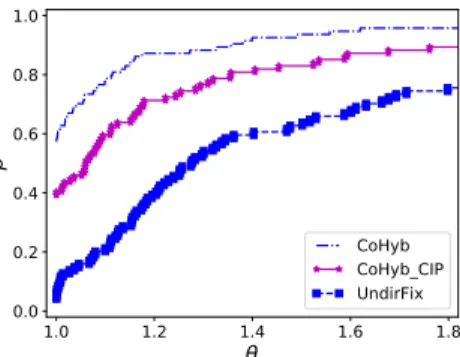
The performance profiles of CoHyb, CoHyb CIP and UndirFix are given in
Fig-701
ure 5.5with the edge cut as the evaluation criterion. As seen in this figure, CoHyb is 702
the best performing variant, and UndirFix is the worst performing variant. This is 703
interesting as in the general setting, we saw a reverse relation. The variant CoHyb CIP 704
performs in the middle, as it combines the other two. 705
5.6. Runtime performance. We now assess the runtime performance of the 706
proposed algorithms. Figure 5.6shows the runtime comparison and distribution for 707
13 graphs with the longest coarsening time for the CoTop variant. A description of 708
these 13 graphs can be found inTable 5.3. InFigure 5.6, each graph has three bars 709
representing the runtime for the multilevel algorithm using the coarsening heuristics 710
described inSubsection 4.1: CoTop, CoCyc, and CoHyb. We can see that the run time 711
performance of the three coarsening heuristics are similar. This means that, the cycle 712
detection function in CoCyc does not introduce a large overhead, as stated in
Sec-713
tion 4.1.2. Most of the time, CoCyc has a bit longer run time than CoTop, and CoHyb 714
offers a good tradeoff. Note that in Figure 5.6, the computation time of the initial 715
partitioning is negligible compared to that of the coarsening and uncoarsening phases, 716
which means that the graphs have been efficiently contracted during the coarsening 717
phase. 718
Figure 5.7 shows the comparison of the five variants of the proposed multilevel 719
scheme and the single level scheme on the whole dataset. Each algorithm is run 10 720
times on each graph. As expected, CoTop offers the best performance, and CoHyb 721
offers a good trade-off between CoTop and CoCyc. An interesting remark is that these 722
three algorithms have a better run time than the single level algorithm UndirFix. For 723
example, on the average, CoTop is 1.44 times faster than UndirFix. This is mainly due 724
to cost of fixing acyclicity. Undirected partitioning accounts for roughly 25% of the 725