HAL Id: hal-00909120
https://hal.inria.fr/hal-00909120
Submitted on 25 Nov 2013
HAL is a multi-disciplinary open access
archive for the deposit and dissemination of
sci-entific research documents, whether they are
pub-lished or not. The documents may come from
teaching and research institutions in France or
abroad, or from public or private research centers.
L’archive ouverte pluridisciplinaire HAL, est
destinée au dépôt et à la diffusion de documents
scientifiques de niveau recherche, publiés ou non,
émanant des établissements d’enseignement et de
recherche français ou étrangers, des laboratoires
publics ou privés.
Cloud
Frédéric Desprez, Jonathan Rouzaud-Cornabas
To cite this version:
Frédéric Desprez, Jonathan Rouzaud-Cornabas. SimGrid Cloud Broker: Simulating the Amazon AWS
Cloud. [Research Report] RR-8380, INRIA. 2013, pp.30. �hal-00909120�
0249-6399 ISRN INRIA/RR--8380--FR+ENG
RESEARCH
REPORT
N° 8380
November 2013SimGrid Cloud Broker:
Simulating the Amazon
AWS Cloud
RESEARCH CENTRE GRENOBLE – RHÔNE-ALPES
Inovallée
Amazon AWS Cloud
F. Desprez
∗, J. Rouzaud-Cornabas
∗Project-Team Avalon
Research Report n° 8380 — November 2013 — 30 pages
Abstract: Validating a new application over a Cloud is not an easy task and it can be costly
over public Clouds. Simulation is a good solution if the simulator is accurate enough and if it provides all the features of the target Cloud.
In this report, we propose an extension of the SimGrid simulation toolkit to simulate the Amazon IaaS Cloud. Based on an extensive study of the Amazon platform and previous evaluations, we integrate models into the SimGrid Cloud Broker and expose the same API as Amazon to the users. Our experimental results show that our simulator is able to simulate different parts of Amazon for different applications.
Key-words: Cloud, SimGrid, Simulation, Amazon Web Service, Performance evaluation, IaaS
d’Amazon
R´esum´e : La validation d’une nouvelle application sur un Cloud n’est pas une
tˆache facile et elle peut ˆetre coˆuteuse sur des Clouds publiques. La simulation
reste une bonne solution si le simulateur est suffisament pr´ecis et qu’il fournit toutes les fonctionnalit´es du Cloud cible.
Dans ce rapport, nous proposons une extension de l’outil de simulation Sim-Grid pour simuler le Cloud publique Amazon. En nous basant sur une ´etude extensive de la plate-forme Amazon et sur des ´evaluations pr´ec´edentes, nous int´egrons les mod`eles dans le SimGrid Cloud Broker et proposons la mˆeme API qu’Amazon. Nos r´esultats exp´erimentaux montrent que notre simulateur est capable de simuler les diff´erents ´el´ements du Cloud Amazon pour diff´erentes applications.
Mots-cl´es : Cloud, Simgrid, Simulation, Amazon Web Service, ´evaluation de
1
Introduction
Using Cloud Computing infrastructures and especially the Amazon Web Service
(AWS)1platform has become a major trend for both commercial and scientific
computing. Large scale data-intensive scientific workloads [6, 10, 14, 15, 17] have been shown to be good candidates for such platforms.
However, many application developpers and scientists want to evaluate if the Cloud is fitting their needs. But porting an application over a Cloud platform and evaluating it at scale comes with a high cost. Resources have to be rent for the time needed to test and run their application. Furthermore if an user wants to evaluate different strategies/algorithms, he/she need to repeat his/her experiments for a period of time that can be quite long. Researchers working on new models for Cloud applications, elastic resource management functions, provisioning algorithms, etc., have the same issue. They need to pay Amazon (or another Cloud provider) for resources they use during development and evaluation processes. Even if Amazon provides scientists with free resources on
their Cloud2, it is still an expensive and tedious way to validate applications.
Furthermore if scientists and application developpers want to optimize their applications, they will pass through numerous fail runs before finding the good trade-offs between multiple parameters such as instance and storage types. For example, using Spot Instances to reduce the cost of a computation has been the subject of numerous studies [35, 36]. These approaches were evaluated on a real Cloud. Accordingly, evaluating and refining them comes with a cost. Moreover AWS is an ever evoling platform and you can not know what other users execute on it. Accordingly when testing different strategies, you are not sure that the underlying platform is the same or what is the overall cost when using spot instances. Thus you can not do reproducible experimentations to compare different strategies on such Cloud. The noise coming from the platform itself and its users will perturbate the results.
Simulation is a simple and efficient approach to validate applications vided that an efficient and accurate simulator exists. In this paper, we pro-pose a multi-Cloud simulator, SimGrid Cloud Broker (SGCB), that provides researchers and engineers with such environments to evaluate their provisioning and elastic algorithms and full applications through simulation before running them on a full fledge Cloud. To avoid complex rewritting of applications, we have adopted the Amazon EC2 and S3 APIs. Thus for someone familiar with these APIs, it is straightforward for her/him to use our simulator. Right now, performance models included in our simulator are based on AWS observations. But they can be changed for any Cloud infrastructure as long as some basic evaluations are available or can be executed as presented in Section 5.3.
This paper is organized as follows. Section 2 gives a short overview of AWS and its main services. Section 3 presents the related work around simulators, performance evaluation of Clouds, and SimGrid. The following section (Sec-tion 4) explains the design of the SimGrid Cloud Broker and finally, before a conclusion and some future work, we explain our evaluation process.
1
http://aws.amazon.com
2
2
Amazon Web Service
Before explaining how we designed and developed our simulator and modeled the AWS infrastructure, we give a short presentation on AWS and the services it provides. From 10,000 feets, AWS is designed around compute (EC2) and storage (S3 and EBS) services.
Elastic Compute Cloud (EC2) EC2 provides computing service through
Virtual Machine abstraction i.e. instance. An instance has access to a set of
resources defined by the instance type 3 it has been instantiated from. The
instance type can be seen as a template of resources: processors’ speed and number, memory, and local storage size. The speed and number of processors are expressed in Elastic Computing Unit (ECU), a processor abstraction. When requesting an instance, the user must specify the instance type he/she wants to use and a disk image (Amazon Machine Image, AMI) that describes where the
operating system and applications are stored4.
Finally, there are three type of EC2 pricing: on-demand, reserved, and spot instances. For on-demand instances, the user pays a flat fee every hour. For reserved instance, the user pays a fee upfront and then a smaller fee than on-demand each hour. Contrary to the others two, the price of spot instances is dynamic and always changing. For spot instances, the user pays a small fee every hour but he must bid on a specific price. His spot instance will run while his bid is higher than the current price of spot instances. His instance will be killed by AWS when the price is higher than his bid. If an instance is killed due to an out of bid, the current hour is free for the user. For all princing schemes, the full hour is paid if the user terminates his instance. There are two policies for spot instances: one-time and persistent. With the one-time policy, the spot instance will be started and if killed, it will not be relaunched. With the persistent policy, spot instances are relaunched everytime the spot instance price is lower to the bidded price.
Simple Storage Service (S3) S3 provides a key-value storage available on each region. Accordingly, we need a set of Physical Machines (pm) in each region to host S3 services. The S3 of each region is available worldwide (from each region and from outside AWS). S3 can be used to store user’s data but also to store Virtual Machine Images. Within AWS, they are named Amazon Machine Image (AMI).
Elastic Block Storage (EBS) EBS provides a block storage. As for S3, it is
available in each region. Furthermore, a EBS Volume, i.e. a remote virtual disk with a quantity of storage reserved by an user, is specific to an availability zone. It can not be used in other availability zones or from outside AWS. EBS Volumes can be either be used for secondary storage and mount within an instance or used as root filesystem for an instance. Furthermore, it is possible to take a snapshot of an EBS Volume and store it into the S3 of the region. In this case,
the snapshot is compressed and the price of storage is specific to EBS snapshot5.
3 http://aws.amazon.com/ec2/instance-types/ 4 https://aws.amazon.com/amis 5 http://aws.amazon.com/ec2/pricing/
This snapshot can then be restored into another EBS Volume. It is not possible to transfer this snapshot to other regions but it can not be seen within S3.
3
Related Work
3.1
Cloud Simulators
Many papers present “experimental” results that have been done using simu-lators built for a specific part of a Cloud and customized for each paper. For example, as most of the work has been done around the mapping between Vir-tual Machines and Physical Machines within a datacenter or a Cloud, simulators try to mimic the behavior of Cloud resource brokers. Thus they can not be used for other target algorithms (involving data management for example). Further-more most of them lack of proper validation processes.
CloudSim [3] has been built upon the existing GridSim framework. It is mainly built to understand the behavior of a Cloud from the Cloud Service Provider point of view. To be able to do that it has to model and simulate Cloud infrastructures, including data centers, users, user workloads, and appli-cation provisioning. But as shown in [25], CloudSim is not scalable and lacks a proper validation process for its network model. CloudAnalyst [34] is built on top of the CloudSim toolkit; it provides visual modeling, easy to use graphical user interfaces, and large-scale application simulations deployed on the Cloud infrastructure. Application developers can use CloudAnalyst to determine the best approaches to allocate resources among available data centers to serve spe-cific requests and determine the related costs for these operations.
CReST [4] is a discrete event simulation toolkit built to evaluate Cloud provi-sioning algorithms. It was used for example to evaluate different communication protocols and network topologies in a distributed platform.
Alberto Nu˜nez et al. introduced in [22] a novel simulator of Cloud
infrastruc-tures called iCanCloud. It reproduces the instance types provided by a given CSP, and contains an user-friendly GUI for configuring and launching simula-tions, that goes from a single VM to large Cloud computing systems composed of thousands of machines. But they simulate a Cloud as viewed by a CSP and not by an Cloud user. Furthermore, they lack a proper validation process for their models and show a limited scalability in term of number of VMs.
GreenCloud [18] targets energy-aware cloud computing data centers. It is build as an extension of NS-2 and focuses on energy consumption at every level of the Cloud architecture.
3.2
AWS Performance Evaluation
A simulator is only useful if its performance model and results have been val-idated over an actual platform and if they are accurate enough. Indeed, the purpose of such a simulator is to closely reflect the environment it simulates. We have started our work by doing an extensive study of previous works on AWS and gathered all the information available at the moment.
Numerous papers present benchmarks and benchmark tool suites for Clouds. CloudCmp [19] proposes to compare different Cloud Service Providers. To do so, it measures the elastic computing, persistent storage, and networking services.
The tools and the data collected while running it are available online 6.
C-Meter [37] allows to measure the time to acquire and release virtual computing resources. It also allows to compare different configurations of Virtual Machines. Many papers [8, 12, 23, 27] study the performance variability of the same VM Template i.e. Instance Type, within AWS. On AWS, few instances are running on dedicated physical machines. Most of them are running on shared ones. Therefore, depending on what the other VMs are doing, performance can dramatically change [31]. Another factor of variability is the underlying hardware on which instances run. The authors of [23] have shown that the same instance type can be running on at least 3 different hardware configurations in the same AWS region. These different hardware configurations can induce up to 60% performance variation. But it is not possible to predict which hardware configuration an instance will get. Furthermore, the underlying hardware of AWS is rapidly changing. Thus, this variability can disappear or be worthen in the near future. Therefore, it is not possible to model such variability and we will not try to do so with our simulator. Our performance model is based on the mean performance observed and the instance type characteristics announced by
AWS7.
3.3
SimGrid
Simulators are often seen as a technical validation mean, and most of the time, a custom tool is developed for each paper. The problem is that most simula-tors have not gone through a proper validation. Accordingly, their accuracy and the reproducibility of their results have not been verified. To avoid these issues, we have implemented our AWS simulator on top of SimGrid [5]. It is an an opensource, generic distributed systems simulation framework providing very realistic and flexible simulation capabilities. SimGrid was conceived as a scientific instrument, thus the validity of its analytical models was thoughtfully
studied [32]. It has been used as simulator in 119 scientific publications8.
4
Designing an Extendable and General
Pur-pose Cloud Simulator
In this section, we first explain how we have modeled the AWS infrastructure and its instances. Then, we explain how we simulate the AWS middleware. Fur-thermore, we show how we manage the accounting of resources. This accounting is then used to replicate the billing process of AWS. Finally, we present the Sim-Grid Cloud Broker user API that emulates S3 and EC2 ones. In this first version of the simulator, we present simple but yet accurate models. Thanks to plugable interfaces for all the models, changing one model or all of them is an easy task. Furthermore, we keep the interface simple enough to ease the implementation of new models. 6 http://cgi.cs.duke.edu/∼angl/ 7 http://aws.amazon.com/ec2/instance-types/ 8 http://simgrid.gforge.inria.fr/Publications.html
4.1
Multi-Clouds Infrastructure Models
To be able to simulate AWS, we first had to model its infrastructure. Based on the knownledge gathered from the AWS website, we present our AWS infras-tructure model. Then we explain how we have modeled the instances and their performance.
4.1.1 AWS Infrastructure Models
The global infrastructure of AWS can be divided into regions. Regions are dis-persed and located in separate geographic areas. At the moment, there are 8 regions in Asia, Australia, Europe, South America, and North America. Fur-thermore, each region contains one or multiple availability zones. Availability Zones are distinct locations within a region that are engineered to be isolated from failures in other Availability Zones and provide inexpensive, low latency network connectivity to other Availability Zones in the same region. Finally we need to include in the model a specific pm that models the user. The user wants to deploy an application to compute and store a set of data. We model it as a pm connected to one or several regions. Based on these knowledges, we have created a general model of AWS presented in Figure 1. Each region is composed of a set of availability zones connected by a 100 GB/s link. Each region is connected to a set of other regions through a set of 100GB/s links. The user is connected to Northern California and Ireland Clouds through a 10 MB/s link. This model can be easily modified based on more fine grain knowledge. For example, through experimentation, it should be possible to have a better knowledge of network links between AWS regions and their bandwidth and la-tency. It can also be used to model any multi-Cloud or federation of Clouds that can be represented as a set of geographic locations that are composed of one or multiple datacenters. Therefore, most of the multi-Cloud infrastructures can be modeled like this.
As we have previously explained (see Section 3.2), we do not try to simu-late the variability due to different hardware configurations. Furthermore, it is impossible to simulate the interference coming from instances run by other users. Indeed, we lack representive traces of AWS workloads. Therefore, we can not model such interference. We simulate that an availability zone has a set of clusters. Each cluster is composed of physical machines. The physical machine configurations reflect the hardware capacity of instance types. As we do not model interference and resource sharing, we run one instance per pm. An instance will be affected to a pm with the same hardware configuration that the instance type it is based on. Therefore, we provide an instance with the exact resources AWS is claiming it gives it. On each computing pm, we run a process that simulates a hypervisor (see Section 4.2.3).
But the computing pm are not the only pm of the AWS infrastructure. We also need pm to run storage. There are two storage services on AWS: Elastic Block Storage (EBS) and Simple Storage Service (S3). At the moment, the S3 service (see Section 4.2.1) needs one pm per region to run and so does the EBS service (see Section 4.2.2). Finally, we need a set of pm to run the other administration services (see Sections 4.2.3 and 4.2.4).
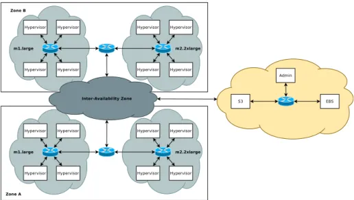
Figure 2 describes how we model a region and its availability zones. For the sake of clarity, we did not include all the instance types available on the
Figure 1: Amazon Web Service Global Infrastructure.
Figure 2: Amazon Web Service Region Infrastructure.
figure but they are available within the simulator. As for the general model, the region model can be easily modified based on more fine grained knowledge. Moreover, the region model can be used to describe any Clouds or part of a Cloud composed by a set of datacenters that share a geographical location. It can also be extended to provide pm to other services such as a load balancer or
a database. Finally, it can be extended to provide pm for new instance types.
4.1.2 Instance Types
As we have previously stated, we do not try to reproduce performance variability as it is not possible to model it. Therefore, the processor power is based on the definition of an EC2 Compute Unit (ECU) given on the Amazon website. One EC2 Compute Unit provides the equivalent CPU capacity of a 1.0-1.2 GHz 2007 Opteron or 2007 Xeon processor. This is also the equivalent to an early-2006 1.7 GHz Xeon processor referenced in our original documentation. Within
SimGrid, processor power are modeled through FLOPS counts9. Therefore, we
have translated 1 ECU to 4.4 GFLOPS as stated in [13]. We do have memory capacity available on our simulator but it is not currently used as SimGrid is not able to simulate memory contention. But it does not change the accuracy of the simulation.
For the local instance storage i.e. local hard drive, a performance model is presented in Section 4.2.3. For the remote block storage i.e. Elastic Block
Storage (EBS) 10, a performance model is presented in Section 4.2.2. For the
network performance, the model is presented in Section 4.1.4
4.1.3 Instance Life Cycle
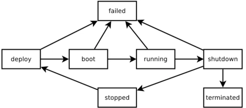
As AWS, we have divided the life cycle of instances into 7 different states: deployed, booted, running, stopped, shutdown, terminated, and failed. The S3-backed instance can not be stopped. Indeed, when in a stopped state, an instance is not allocated to a pm but its disk is kept. The disk of S3-backed instance are volatile, i.e. it is stored on the local disks of a pm when the instance is in the running state but destroyed when shutdown. Accordingly, the stopped state is only available for the EBS-backed instances, i.e. EBS is a persistent disk and can be kept even after an instance went through the shutdown state. Therefore, only EBS-backed instances have the ability to be stopped and restarted. Other instances can only be started once and terminated. Figure 3 displays the complete life cycle of an instance.
Figure 3: Life cycle of an instance. 9
FLOPS: FLoating-point Operations Per Second
10
When an user requests an instance, it is marked as deployed. The deploy-ment process on Amazon EC2 has been deeply studied in [20]. In our simulator, the first step of a deployment process consists in selecting an available pm (see Section 4.2.3). Depending on the storage instance, the deployment is different. For S3-backed instance, the AMI is downloaded to the selected pm from the S3 storage specified in the AMI metadata. In [20], the authors have conducted an extensible study of instance startup time on AWS and other Clouds. As in [13], the authors observe that multi-instance requests i.e. requesting more than one instance at a time, do not impact the startup time. Furthermore the instance type does not impact the startup time. The startup time is the same in all AWS regions and at all time of a day.
As observed in [20], the main impact on startup time is the size of the AMI. Therefore, it is the transfer between S3 and the pm where the instance will be started that impacts the startup time. As multi-instance requests do not impact startup time, the bandwidth limitation is by flow as also observed in the two other studies. Accordingly, we use the model presented in Section 4.2.1 to limit the rate of each flow between instances or pm and S3 service.
As explained in Section 4.2.3, the startup time is longer as spot instance management service only verifies if there are some spot instances to start every 5 minutes. Therefore, in the worst case, it adds 5 minutes to the startup time. This is done to mimic AWS as observed in [20].
For EBS-backed instances, the EBS Snapshot specified in the AMI meta-data is used to create a new EBS Volume (see Section 4.2.2). Then, the EBS Volume is mounted on the selected pm. Therefore, the EBS service must load the snapshot from the S3 service. We apply the same performance model than between pm and S3 service i.e. a 10.9 MB/s bandwidth limitation.
When the instance disk has been uploaded to the selected pm or when the root EBS volume mounted, the instance can be booted. As observed in [20], the boot time depends of the operating system, i.e. Linux or Windows. We could easily support both but we focus on Linux in this work. Moreover as previously explained, the instance type has almost no impact on the boot time. Accordingly, we simulate the boot time as a static number of seconds. The boot time contains the Operating System boot time and the virtualization layer creation time. From the observation given in [13, 20], we have set this value to 96 seconds.
When the instance has finished to boot, its state changes to running. When running, an instance can receive SimGrid tasks that simulate network interac-tions such as remote command execution or application invocation (see Sec-tion 4.2.3).
When the user requests it (or when a spot instance is out of bill), the instance is shutdown and terminated. As for startup time, multi-instance requests, in-stance types, time of the day, or AWS region do not impact the release time, i.e. termination of an instance. Therefore, as release time is the time to shutdown the Operating System and remove the virtualization layer at the pm level, we have modeled it as a static variable. Through observation gathered from [13, 20], we have set this value to 6 seconds.
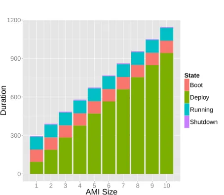
Figure 4 shows our simulated life-cycle of multiple instances with different AMI sizes. As one can see, the results are similar than the one observed on AWS and reported in [20].
0 300 600 900 1200 1 2 3 4 5 6 7 8 9 10
AMI Size
Dur
ation
State Boot Deploy Running ShutdownFigure 4: AWS Middleware Simulation.
any moment. In this case, the instance is shut down and put in the stopped state. The related EBS volume is not destroyed and the instance can be restarted later. Furthermore, when in a stopped state, an instance is not allocated to a given pm. To be restarted, the instance goes back to the deployment state but a new EBS Volume is not created but the old one is mounted to the newly selected pm and the instance is booted again. Accordingly, when an instance is stopped and restarted, it can have moved from a pm to another one.
At any moment, an instance state can change to the failed one. It describes any faults that renders the instance not working. It can happen if the registred AMI is incorrect, if the network transfer failed during the deployment state, pm has crashed, etc..
4.1.4 Instance Network Connectivity
On AWS, one instance is only useful if it is possible to connect to it through network. Indeed a large part of the AWS instances are used for Web Services thus they must be accessible through the Internet. Furthermore, deploying AWS is used to deploy n-tier web applications and scientific applications. Most of the time, these services use multiple instances that communicate. Accordingly, it is critical to model the network performance on AWS. As we have built our simulator on top of SimGrid, we already benefit from its accurate network model. Nonetheless we need to calibrate the bandwidth between the instances and between the instances and the outside world.
AWS network performance have studies numerous times [8, 19, 33]. Using them, we deduced a network bandwidth between instances in the same region of 75 MB/s and an inter-region (and Internet) bandwidth of 37.5MB/s. This
model does not take into account the cluster compute instances with larger network bandwidth. For network storage, i.e. S3 and EBS, we have other network models presented in Sections 4.2.1 and 4.2.2.
4.2
Cloud Middleware Simulation
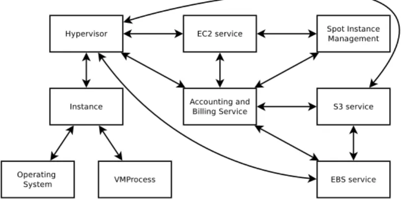
In this section, we present how we emulate the different services that compose the AWS middleware. First, we show how we added a virtualization layer on top of SimGrid with complete hypervisor and Virtual Machine abstractions. Then we show how we are able to simulate storage services and the related performance models. Finally, we show how we extended SimGrid to do real-time resource accounting and used it to emulate the billing process of AWS. Figure 5 presents our AWS middleware simulation and how the different services are inter-connected. We now explain each of these services.
Figure 5: AWS Middleware Simulation.
4.2.1 Simple Storage Service
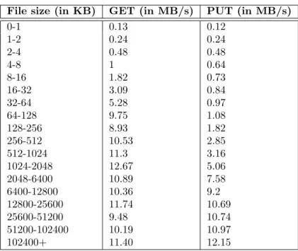
The S3 simulation is straightforward. It emulates a key-value storage with ob-jects stored into buckets. From a simulation point of view, we are not interested by the actual data stored into each object. We are only interested by its size. Accordingly, we just manage a set of buckets that contain a set of objects of a given size. As the software that builds S3 is not available and as we do not know on which hardware it runs, we were not able to construct an advanced performance model. We threated S3 as a blackbox and we only observed it from the outside, i.e. by interacting with the S3 API. Based on multiple studies such as [11, 24, 26], we used the performance model presented in Table 1. Our model only threats mono-thread interaction with S3. We do not try to model multiple threads ones.
The user can interact with S3 trough its API. Other services such as EBS are also interacting with S3 through its API.
4.2.2 Elastic Block Storage
As one can see in Figure 2, an EBS service is available per region. But as we previously stated, the EBS volumes are specific to an availability zone. We
File size (in KB) GET (in MB/s) PUT (in MB/s) 0-1 0.13 0.12 1-2 0.24 0.24 2-4 0.48 0.48 4-8 1 0.64 8-16 1.82 0.73 16-32 3.09 0.84 32-64 5.28 0.97 64-128 9.75 1.08 128-256 8.93 1.82 256-512 10.53 2.85 512-1024 11.3 3.16 1024-2048 12.67 5.06 2048-6400 10.89 7.58 6400-12800 10.36 9.2 12800-25600 11.74 10.69 25600-51200 9.48 10.74 51200-102400 10.19 10.97 102400+ 11.40 12.15
Table 1: I/O Performance model for S3.
enforce this separation at the service level. An EBS Volume can only be mounted by one instance at a time. This limitation is also enforced at the service level.
The EBS service provides an API that deals with the creation, modification, and deletion of an EBS Volume. It also provides API call to snapshot an EBS Volume and to restore it into an EBS Volume. Furthermore, API calls are available to mount the EBS Volume as root or secondary hard drive for a given instance. The API is used by the hypervisors and by the EC2 middleware. To store and retrieve snapshots, EBS interacts with the S3 service. Snapshots are stored into a specific bucket (snapshot) that does not appear when a user lists its bucket within S3. An EBS service only interacts with the S3 service of its region.
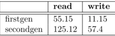
As S3, EBS is not a service based on an available software and we do not know on which hardware it runs. Accordingly, we were not able to construct an advanced performance model. We threated EBS as a blackbox and only we observed it through the outside i.e. within an instance that uses a EBS Volume. Due to better network performance, EBS I/O performance are not the same on all instance types. As for local disk, we have two models: one for small, medium, and first generation (m1) instance types and one for second genera-tion (m2) instance types. For the moment, we have not tried to model I/O performance of RAID array composed of multiple EBS Volume. Our model is presented in Table 2.
4.2.3 Compute
The Elastic Compute Cloud service is simulated through 4 different compo-nents within SGCB: hypervisor, instance, operating system, and EC2 service.
read write
firstgen 55.15 11.15
secondgen 125.12 57.4
Table 2: I/O Performance model for EBS Volume (in MB/s).
Together, they provides the same services than an IaaS middleware such as
OpenNebula [21] or OpenStack11.
EC2 Service The EC2 service manages the AMI, the different instance types, the placement of instances on pm, etc. It implements all the management tasks behind the EC2 API. Accordingly, it has a catalog of all registered AMI and where the related operating system and applications are stored. It also has a catalog of all available instance types and their related capacities and prices. It has a list of all pms of a region and which ones are available, i.e. on which no instance is running. It is in charge of the placement of instances on pm. It keeps a list of instances where they are running, in which state they are in their life cycle. It interacts with other services (EBS and S3) to provision instances and their related data to the selected hypervisor. As for EBS service, EC2 service enforces a set of limitations. For example, AWS users can not request more than 10 on-demand and 50 spot instances. EC2 service enforces this limitation. A part of the EC2 service is externalized into another service: Spot Instance Management (SIM). This service is dedicated to manage spot instances life-cycle and their dynamic prices. Based on spot instances requests and the related bid provided by the user, the spot instance management starts and kills spot in-stances depending of the dynamic price. This dynamic price can be simulated through tree strategies: random, file, and model. The random strategy is quite simple. The dynamic price is set to 40% of the price of on-demand instances. Then every 5 minutes, the price is incremented or decremented by a value be-tween 0 and 0.01. The file stragegy replays a price trace from a file. We use a csv to store the trace (date, price). The model strategy implements the model presented in [1]. It is also possible to add new strategies e.g. the model pre-sented in [16]. Finally, every 5 minutes, the SIM service checks if there is some spot instances to start or terminate.
Hypervisor The hypervisor receives commands from the EC2 service to start,
stop, and manage the instance hosted on the pm where it runs. Accordingly, the hypervisor fetches from S3 the operating system and the applications, i.e. the set of objects linked to the AMI. It can also request to mount an EBS Volume to an instance by interacting with the EBS service. It launches the instance i.e. the VM abstraction and the operating system inside it. It mounts or unmounts secondary EBS volumes to the instance. And it can stop an instance and the related operating system. Finally, it gathers accounting data from the instance and sends it on request to the accounting service (see Section 4.2.4).
11
read write
moderate 81.03 45.85
m1.high 481.67 149.44
m2.high 690.41 242.84
Table 3: I/O Performance model for local disks (in MB/s).
Instance Instance is an extension of the virtualization layer of SimGrid, i.e.
VM. Within SimGrid, a VM is a container that contains a set of processes. An instance has always an Operating System process and a set of VMProcesses.
An instance provides an I/O abstraction to read/write on disk. Depending if the operation happen on a local or a remote (EBS) disk, it applies different performance models. For the local (ephemeral) disk, there are different I/O
performance policies 12 depending of the instance type. But even if first and
second generation instances with high I/O performance must have similar I/O performance, we have observed the opposite. Based on data gathered by
Cloud-Harmony13, we have differenciated three local disk performance models: one for
small and medium instance types (moderate), one for m1 large and xlarge ones (m1.high) and one for m2 xlarge, 2xlarge and 4xlarge instance types (m2.high). As explained in [13], local disks have a buffer in memory. Our model does not take it into account. Therefore, we only model the direct I/O to the local disk. It is displayed in Table 3.
For EBS disk, a message of the size of the data is sent to the EBS service. The EBS performance model is presented in section 4.2.2.
The VMProcesses are similar to SimGrid processes but they expose a virtual network abstraction allowing instances to send and receive messages.
Operating System The Operating System (OS) process is a VMProcess with
a set of functions to receive and send messages and to execute processes. First of all, the OS process simulates the boot time as described in Section 4.1.3. The OS can receive special messages that request to load and execute an application. It is also aware of the availability of secondary EBS storage and mounts them. It provides two other services: one to package and send the root directory to S3 and another one to load a S3 object into a mounted disk (local or remote).
4.2.4 Accounting and Billing
As we previously explained, accounting is critical to simulate a Cloud. As we want to provide a full simulation of AWS, we need to account all the resources that are billed by it. Accordingly, on top of accounting how many instances of each instance type and the chosen pricing model, we need to account the quantity of S3 and EBS storage and all the network traffics.
The Account and Billing Service (ABS) interacts with EC2 Service to gather knowledge about the running instances. When an instance has run for an hour, it is billed to the user. When an instance is terminated, it is billed to the user as a full hour even if not all the time has been consummed (as AWS does).
12
http://aws.amazon.com/ec2/instance-types/
13
For the storage, every 5 minutes, ABS contacts S3 and EBS services and retrieves the amount of data stored. It needs the size of all the objects stored in S3, the size of reserved EBS Volume and the size of all EBS snapshots. At the end of every hour, it selects the maximum size used during the hour e.g. if an user has used 10GB of S3 storage during 20min and then 5GB during 40min, it will select 10GB. Then it converts it into Byte-Hour e.g. 10GB/H in this example. It sums this value to the amount of Byte-Hour already used during the previous hour. At the end of a month or the simulation, it converts the Byte-Hour into GB-Month metric. By doing so, we replicate the behavior of
AWS 14. We apply the same process for EBS and EBS snapshots. Therefore,
we have three GB-Month variables one per type of storage.
For the data transfer, we need to account the amount of traffic for four differ-ent types of transfers: intra-availability zone, intra-region i.e. inter-availability zone within a region, and internet, i.e. inter-region, and transfer coming or going to pm outside of AWS. To do so, we have extended S3 service and the virtualization layer (hypervisor, instance and VMProcesses) to log the size of every messages they send/receive and where they send/receive it. When an instance is asked, it aggregates all the message sizes and destinations into a table containing the destination and the total amount of data send to. Every 5 minutes, ABS asks each hypervisor to send the network accounting data. The hypervisor gathers these information from the instance and sends them back to ABS. Then, ABS does the same for S3. Using all the network accounting data, ABS reconstructs all the network traffic. Then it classifies it depending where it comes from/to: the same availability zone, region, other regions, or Internet.
By using the information gathered from EC2 15 and S3 pricing pages 16
and all the information gathered by ABS, we are able to replicate AWS’ billing policy.
4.3
User interfaces
Replicating EC2 and S3 API To ease the usage of our simulator, we have
implemented the EC2 and S3 APIs. Accordingly, EC2 and S3 services presented in Sections 4.2.3 and 4.2.1 provide an interface similar to REST API. The syntax
of these REST calls are similar to the one described in the EC2 17 and S3 18
API reference. As for AWS, a REST API interface is available for each region. Accordingly, an SGCB user will see AWS as a set of EC2 and S3 API interfaces that are the same as the Amazon ones. As for AWS, the user can request real-time accounting data to know what he/she has consumed and what is it billed in each region. For example, these data can be used by adaptive provisioning algorithms to enforce a given budget.
Experimental Scenarios To furthermore ease the simulation of an
applica-tion, we have implemented a experimental scenario life-cycle. Indeed, most of the application on a Cloud have the same life-cycle that can be divided into
14
http://aws.amazon.com/s3/faqs/#How will I be charged and billed for my use of Amazon S3 15 http://aws.amazon.com/ec2/pricing/ 16 http://aws.amazon.com/s3/pricing/ 17 http://docs.aws.amazon.com/AWSEC2/latest/APIReference/query-apis.html 18 http://docs.aws.amazon.com/AmazonS3/latest/API/APIRest.html
Figure 6: AWS Experimental Scenario
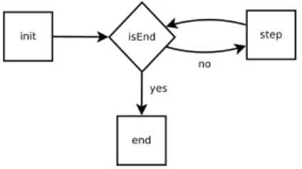
four states as presented in Figure 6. When each scenario begins, there is no instance or AMI within AWS. Accordingly, it is requested to do all the steps of deploying an application. It brings a complete view of the cost and complex-ity of the deployment of a new application in AWS. The first state (init) is a provisioning and configuration process. The user selects a set of instances and their storage and requests them on one or more regions. Then he/she deploys his/her application on them. The second state (isEnd) is a conditional state. The scenario checks if the ending condition is true, for example, if the appli-cation has finished to process all its tasks or if a deadline is reached. If the ending condition is false, the scenario goes to the third state (step). During this state, the scenario verifies if the application has enough resources and if it needs to add more resources or delete some of them. Accordingly this state im-plements the elasticity function related to the application. The last state (end) is reached if the ending state is true. This state is important as it must properly shutdown the application and releases all the resources it has used. Indeed if not all resources have been released, the user will continue to pay for them.
For example, a basic Bag of Tasks scenario can be to run 10 stateless service with the cheapest m1.large instance type. The ending condition is reached if all the 1,000 tasks are processed by an instance of the stateless service. In the init state, the scenario selects the region that provides the cheapest price for m1.large spot instances. Then, it uploads the operating system and the application to the S3 storage of the region. Only after doing it, the scenario can register the AMI and request 10 m1.large spot instances of this AMI. The scenario goes to the isEnd state. It checks if all the tasks have been sent. If it is not the case, it goes to the step state. By checking the state of each instance, it can verify which one are running. If they are running, it can send a set of tasks to process and fetch the results of the completed tasks. When the result of a task is fetched from an instance, the tasks is marked as done. During the step state, the scenario can also request to check if another region is now cheaper than this one. If it is the case, all the spot instances are canceled and new ones are requested in the new region. Warning, an AMI is specific to a region thus the upload and register of an AMI must be done within each region. When the isEnd state is true i.e. all the tasks have been processed and the results fetched, the scenario goes to the end state. The scenario must release all the spot instances, delete the AMI and the related S3 objects.
4.3.1 Building PaaS and SaaS Simulations on Top of SGCB
We have presented how SGCB can be used to test provisioning algorithms and simulate applications on top of AWS. Using the different SGCB services, it is
possible to create a set of VMProcesses that will run other VMProcesses, e.g. for simulating a PaaS or a composition of VMProcesses distributed onto different instances, e.g. a SaaS application. Therefore, SGCB is able to simulate any application that is running on top of AWS and can be extended to simulate PaaS and SaaS Cloud.
4.3.2 Traces and Post-Analysis
SimGrid already provides a large set of visualisation tools [28, 29, 30] to ease the analysis of simulation runs. We also have extended the tracing module of SimGrid to take into account virtualization and AWS services. Accordingly, it is possible to retrieve all the state of an instance life cycle in the trace. The spot instance dynamic price changes are also available within these traces. All the accounting data are traced at each step of the simulation. We provide a set of R scripts that are able to analyze the traces and we used them to produce the figures of Section 5. They can reconstruct the different parts of the bill (network, compute, storage) for each region. It is also possible to see the time for each state of the instance lifecycle and the time taken to run each VMProcess. This trace can be compared with real AWS traces to validate the simulation and modify the different models (AWS ones and the application one) to increase the accuracy.
For example, for the Bag of Tasks scenario, it is possible to reconstruct how many tasks have been computed by each instance and compute the price per task. Furthermore, the trace can be compared with a run on AWS and use to improve the accuracy of the performance model of these tasks on different instance types.
5
Evaluation
To evaluate our simulator, we wrote some basic examples. The purpose is to demonstrate the easiness to use it and the large spectrum of functionalities available. In Section 5.1, we show that it is easy to test a large set of basic AWS tasks. Moreover, we present a simple Bag of Tasks application to describe how a complete application can be simulated in Section 5.2. Furthermore, we show how the traces can be used to easily compare the cost and performance of different resource reservation policies. In Section 5.4, we show that we are able to simulate even the larger applications that run on AWS. Finally, we explain how SGCB can be extended to support other instance types, AWS regions, and services in Section 5.3. Moreover, we also describe in this section how other Cloud platforms such as HelixNebula, could be simulated within SGCB.
5.1
Expressivness
Uploading and downloading data to/from S3 can be done by writing only few lines of Java. In Listing 1, we show how to create a bucket (line #1-4) and upload an object into it (line #5-8). On line #1, we create a new S3 REST-like call. Then, we declare that this call will be a CreateBucket call (line #2) to create a bucket (testBucket). On line #3, we send it. The S3 service sends its response of the call and it is received on line #4. Then, we do the same but to
upload (PutObject) an object (testObject) of size (objectSize) into the bucket (testBucket). Lines #3 and #7 show that we interact with the eu 1 region.
Listing 1: Creating a bucket and uploading an object into it.
✞ ☎
1 S 3 C a l l c a l l B u c k e t = new S 3 C a l l ( ) ; 2 c a l l B u c k e t . C r e a t e B u c k e t ( ” t e s t B u c k e t ” ) ; 3 c a l l B u c k e t . i s e n d ( ”S3CONTROLER eu 1” ) ;
4 S3Reply r e p l y B u c k e t = ( S3Reply ) Task . r e c e i v e ( ) ; 5 S 3 C a l l c a l l = new S 3 C a l l ( o b j e c t S i z e ) ;
6 c a l l . PutObject ( ” t e s t B u c k e t ” , ” t e s t O b j e c t ” , new S 3 O b j e c t ( ” t e s t O b j e c t ” , o b j e c t S i z e ) ) ;
7 c a l l . i s e n d ( ”S3CONTROLER ”+cloudName ) ; 8 S3Reply r e p l y = ( S3Reply ) Task . r e c e i v e ( ) ;
✝ ✆
The same approach of REST-like calls is available for interacting with EC2. In Listing 2, we show how to acquire on-demand instances for the us west 1 region. From lines #1 to #9, we upload the instance image to S3. Lines #11-14 are responsible to register the AMI (testImage) that use the previously uploaded image (testObject in the bucket testBucket). Finally, we start one
m1.smallinstance (lines #16-19).
Listing 2: Acquiring one m1.small on-demand instance from us west 1
✞ ☎
1 S 3 C a l l c a l l B u c k e t = new S 3 C a l l ( ) ; 2 c a l l B u c k e t . C r e a t e B u c k e t ( ” t e s t B u c k e t ” ) ; 3 c a l l B u c k e t . i s e n d ( ”S3CONTROLER us west 1” ) ; 4 S3Reply r e p l y B u c k e t = ( S3Reply ) Task . r e c e i v e ( ) ; 5
6 S 3 C a l l c a l l = new S 3 C a l l ( o b j e c t S i z e ) ;
7 c a l l . PutObject ( ” t e s t B u c k e t ” , ” t e s t O b j e c t ” , new S 3 O b j e c t ( ” t e s t O b j e c t ” , o b j e c t S i z e ) ) ;
8 c a l l . i s e n d ( ”S3CONTROLER us west 1” ) ; 9 S3Reply r e p l y = ( S3Reply ) Task . r e c e i v e ( ) ; 10
11 EC2Call c a l l R = new EC2Call ( ) ;
12 c a l l R . r e g i s t e r I m a g e ( ” t e s t B u c k e t ” , ” t e s t O b j e c t ” , ” t e s t I m a g e ” ) ; 13 c a l l R . i s e n d ( ”EC2CONTROLER us west 1” ) ;
14 EC2Reply r e p l y R = ( EC2Reply ) Task . r e c e i v e ( ) ; 15
16 EC2Call c a l l = new EC2Call ( ) ;
17 c a l l . r u n I n s t a n c e s ( 1 , r e p l y R . g e t A t t r ( ) . g e t ( ” imgId ” ) , ”m1 . s m a l l ” , n u l l ) ; 18 c a l l . s e n d ( ”EC2CONTROLER us west 1” ) ;
19 EC2Reply r e p l y = ( EC2Reply ) Task . r e c e i v e ( ) ;
✝ ✆
Instead of acquiring on-demand instances, it is possible to request spot in-stances. Lines #1-14 of Listing 2 remain unchanged. Only the lines #16-19 are replaced by the one presented in Listing 3. Unlike on-demand instances, spot instances request a bidding price (set to 0.12 here) and a spot instance policy (persistent here).
Listing 3: Acquiring one m1.small spot instance from us west 1
✞ ☎
1 EC2Call c a l l = new EC2Call ( ) ;
2 c a l l . r e q u e s t S p o t I n s t a n c e s ( 0 . 1 2 , 1 , ”m1 . s m a l l ” , r e p l y R . g e t A t t r ( ) . g e t ( ” imgId ” ) , n u l l , ” p e r s i s t e n t ” ) ;
3 c a l l . i s e n d ( ”EC2CONTROLER us west 1” ) ;
✝ ✆
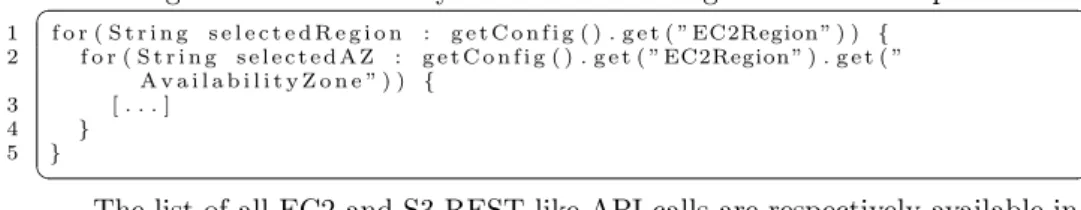
By just adding a loop, such as the one presented in Listing 4, it is possible to do request in multiple availability zone (line #2) and/or AWS region (line #1). Accordingly, testing multi-availability zones and multi-region scenario are easy within SGCB.
Listing 4: Multi-availability zones and multi-regions instance acquisition ✞ ☎ 1 f o r ( S t r i n g s e l e c t e d R e g i o n : g e t C o n f i g ( ) . g e t ( ” EC2Region ” ) ) { 2 f o r ( S t r i n g s e l e c t e d A Z : g e t C o n f i g ( ) . g e t ( ” EC2Region ” ) . g e t ( ” A v a i l a b i l i t y Z o n e ” ) ) { 3 [ . . . ] 4 } 5 } ✝ ✆
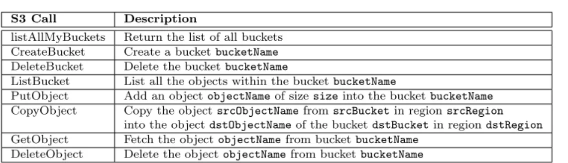
The list of all EC2 and S3 REST-like API calls are respectively available in Tables 4 and 5.
EC2 Call Description
describeInstances Return a list describing all the instances of an user (or a list or only one) describeImages Return a list describing all the AMIs
of an user (or a list or only one) describeTemplates Return a list describing all the
instance types (or a list or only one) (not an official EC2 API call) describeTemplatesPrice Return a list describing all the
instance type on-demand prices (or a list or only one) (not an official EC2 API call)
rebootInstances Reboot one (or multiple) started instance(s) runInstances Start nbInstances of a instanceType
instance types using an AMI imageId and a list of requirement listRequirement
such as the availability zone.
startInstances Start one (or multiple) EBS-backed instance(s) that was (were) stopped.
stopInstances Stop one (or multiple) EBS-backed instance(s) that was (were) started.
terminateInstances Terminate one (or multiple) running instance(s). requestSpotInstances Request nbInstances of a instanceType
instance types using an AMI imageId and a list of requirement listRequirement such as the availability zone with a bid of spotPrice
cancelSpotInstanceRequests Cancel one (or multiple) Spot Instance requests describeSpotInstanceRequests Return a description of all (one or a list)
of spot instance requests
describeSpotInstancePrices Return a description of one (or a list)
of Spot Instances prices for one or multiple instance types. createSnapshot Create a snapshot of an EBS Volume ebsId.
deleteSnapshot Delete a snapshot snapshotId.
describeSnapshots Return a description of one (or a list) snapshots. createVolume Create an EBS Volume of size MB and
optionally populate it with a snapshot snapshotId and within a specific availability zone zone
deleteVolume Delete the EBS Volume ebsId
attachVolume Attach the EBS Volume ebsId to the instance vmId detachVolume Detach the EBS Volume ebsId from the instance vmId describeVolumes Return a description of one (or a list) EBS Volume. registerImage Register an AMI imgName with data located in
s3bundleobject in the bucket s3bucket deregisterImage Deregister the AMI imgId
getBill Return the description of the current bill (overall and per resource types)
(not an official EC2 API call)
S3 Call Description
listAllMyBuckets Return the list of all buckets CreateBucket Create a bucket bucketName DeleteBucket Delete the bucket bucketName
ListBucket List all the objects within the bucket bucketName
PutObject Add an object objectName of size size into the bucket bucketName CopyObject Copy the object srcObjectName from srcBucket in region srcRegion
into the object dstObjectName of the bucket dstBucket in region dstRegion GetObject Fetch the object objectName from bucket bucketName
DeleteObject Delete the object objectName from bucket bucketName
Table 5: S3 API Calls.
5.2
Application Simulation
To demonstrate how to simulate a full application, we take a simple Bag Of
Tasks one. For example, New York Time TimesMachine19 is such application
and has been runned on AWS. In [9], the author explains how they processed a large amount of TIFF images into PNG images. The application is described in Figure 7. The purpose of the application is to run computing tasks sent by the user. First, the user sends (1) a task to the Central Service (CeS). Then, he uploads (2) the input file of the task in the Input Storage (InS). A Compute Service (CoS) fetches (3) a computing tasks and the related input file (4). After computing it, CoS sends (5) the result to the Output Storage (OuS). Finally, the user fetches (6) the results from the OuS.
Figure 7: Simulation of a complete Bag of Tasks application.
Provisioning resources for such application can be done through the combi-nation of multiple services. Our purpose here is not to be comprehensive but to show the expressivness of SGCB. We do neither try to have efficient pro-visioning algorithms. Accordingly, we only use 1 m1.xlarge instance for CoS
19
od_ebs_ebs od_ebs_local od_ebs_s3 od_local_ebs od_local_local od_local_s3 od_s3_ebs od_s3_local od_s3_s3 si_ebs_ebs si_ebs_local si_ebs_s3 si_local_ebs si_local_local si_local_s3 si_s3_ebs si_s3_local si_s3_s3
0e+00 5e+05 1e+06
Duration Scenar io State Start RequestVM SendTasks ReceiveResults TerminateVM End
Figure 8: Makespan of SimpleBoT for each scenario.
and 5 m2.2xlarge instances in the eu 1 region. Furthermore, all the computing tasks have an input file of 1GB and an output file of 500MB. The user always sends 1,000 tasks in one burst at the beginning. The application stops when the results of all the tasks have been fetched by the user. The whole application and its performance model have been coded with 300 lines of Java code.
We have evaluated 18 strategies for this application. For every strategy, CeS is using an on-demand instance. We have evaluated all the combinations of storage for input and output data, i.e. storing the data on the local disk (local), on a EBS volume (ebs), or on a S3 storage (s3). The selected storage can be different (or the same) for input and output data. Furthermore, we have used on-demand (od) or spot instances (si) for CoS. In the following figures, the name of each strategy is built as follow: the type of instances used for CoS, the storage for input data, and the one for output data.
Thank to the trace and a custom R library, we can easily compare the different scenarios. In Figure 8, we can see that the makespan is almost the same for all the scenarios. But by looking of the per-task makespan shown in Figure 9, we can see the impact of the scenario on the processing of each individual task. The other important point is to be able to compare the impact of the scenario on the cost of running the application. In Figure 10, we can see that the biggest part of the bill is due to running instances. Storage and network transfert costs are much smaller. As it could be predicated, it is cheaper to use Spot Instances even if they are less reliable. Using these figures, the process of selecting the proper resource allocation policies is facilitated and the user can select the one that fits his needs. It also goes further and looks for the storage and network consumption for each scenario as shown in Figures 11 and 12.
Furthermore, it is possible to go deeper in the application execution. For example, if the goal is to evaluate an elasticity function, it is possible to generate a figure showing the number of running instances for each period in the Cloud
od_ebs_ebs od_ebs_local od_ebs_s3 od_local_ebs od_local_local od_local_s3 od_s3_ebs od_s3_local od_s3_s3 si_ebs_ebs si_ebs_local si_ebs_s3 si_local_ebs si_local_local si_local_s3 si_s3_ebs si_s3_local si_s3_s3 0 500 1000 1500 Duration Scenar io State SendInput ReceiveInput WriteInput ExecuteTask ReadOutput SendOutput ReceiveOutput
Figure 9: Makespan of each task with SimpleBoT for each scenario.
od_ebs_ebs od_ebs_local od_ebs_s3 od_local_ebs od_local_local od_local_s3 od_s3_ebs od_s3_local od_s3_s3 si_ebs_ebs si_ebs_local si_ebs_s3 si_local_ebs si_local_local si_local_s3 si_s3_ebs si_s3_local si_s3_s3 0 500 1000 1500 2000 Price Scenar io Type EBS Network S3 Network VM S3 VM OD VM SI
Figure 10: Cost of running SimpleBoT for each scenario.
e.g. every hour. It is possible to specialize the figure by adding the number per instance types and/or per region. An example is shown in Figure 13. Finally, the trace also stores the evolution of spot instance prices during the simula-tion. Accordingly, it is possible to create a figure displaying them as shown on Figure 14 or even to do statistical analysis on them.
EBS S3 0 500 1000 GBMonth T ype Scenario od_ebs_ebs od_ebs_local od_ebs_s3 od_local_ebs od_local_local od_local_s3 od_s3_ebs od_s3_local od_s3_s3 si_ebs_ebs si_ebs_local si_ebs_s3 si_local_ebs si_local_local si_local_s3 si_s3_ebs si_s3_local si_s3_s3
Figure 11: Accounting of the storage consumption of SimpleBoT for each sce-nario.
Internet Network VM Intranet Network VM Network S3
0e+00 2e+11 4e+11 6e+11
GB T ype Scenario od_ebs_ebs od_ebs_local od_ebs_s3 od_local_ebs od_local_local od_local_s3 od_s3_ebs od_s3_local od_s3_s3 si_ebs_ebs si_ebs_local si_ebs_s3 si_local_ebs si_local_local si_local_s3 si_s3_ebs si_s3_local si_s3_s3
Figure 12: Accounting of the network consumption of SimpleBoT for each sce-nario.
5.3
Extendability
All the AWS configuration is done through a XML file. By extending this file, it is possible to modify the capacities of each instance type, their prices but also add new ones. For example, to add a new instance type, it only takes three
asia_1 eu_1 usa_east_1 usa_west_1 1 2 3 4 5 6 7 8 9 10 9 10 11 12 13 9 10 11 12 13 9 10 11 12 13 9 10 11 12 13 Hour Number of VM Template m1.large m2.xlarge
Figure 13: Number of running instances for each instance type at each hour in each region.
m1.small m1.large m1.xlarge m2.xlarge m2.2xlarge m2.4xlarge c1.medium c1.xlarge
0.0 0.5 1.0 1.5 0 100 200 300 0 100 200 300 0 100 200 300 0 100 200 300 0 100 200 300 0 100 200 300 0 100 200 300 0 100 200 300 Hour Pr ice Region brasil_1 asia_2 asia_1 eu_1 usa_east_1 usa_west_1 usa_west_2
Figure 14: Evolution of spot instance prices during a simulation.
lines of XML. In Listing 5, we show how to add a new instance m4.2xlarge with 34.2GB of RAM, 8 VCPU of 3.25 ECU and 850GB of local disk with a cost of 2.21$ per hour. By modifying and/or extending the XML file, it is possible to change the whole billing policy for compute, storage, and network resources.
0 2000 4000 6000 8000 0 10000 20000 Number of started VMs Ex
ecution time (in seconds)
Figure 15: Scalability of SimGrid Cloud Broker.
Listing 5: Adding a new instance type
✞ ☎ 1 <i n s t a n c e i d=”m4 . 2 x l a r g e ” vcpu=” 8 ” c o m p u t i n g u n i t=” 3 . 2 5 ” memory=” 34200 ” d i s k=” 850 ”> 2 <o n d e m a n d p r i c e p r i c e=” 2 . 2 1 ” /> 3 </ i n s t a n c e> ✝ ✆
The hardware infrastructure is described in another XML file. For the in-frastructure description, we reuse the SimGrid platform file [2]. Accordingly, we are able to describe any large scale distributed platforms. From a SGCB point of view, it allows us to easily add new regions and services.
5.4
Scalability
To evaluate the scalability of SGCB, we ran multiple simulations with an in-creasing number of instances, i.e. between 1 and 30,000. As from a SGCB point of view, it does not cost more resources to run a small or a very large instance types, all the instances were using the same instance types. In Fig-ure 15, we show the execution time to run one month of simulated time with different numbers of VMs. As one can see, the execution time is linear with the number of instances. With 10,000 VMs and more, the larger execution time can be explained by an increasing cost of sending messages on large platforms with SimGrid. Accordingly, SGCB has a very good scaling factor and is able to easily simulate the larger applications that run on AWS.
6
Conclusion
We have designed a new Cloud Simulator to ease the evaluation of applications on Cloud and the related elastic and provisioning algorithms. Our goal is to
provide a simulation of a Cloud and multiple Clouds as seen by a Cloud User. As most of the interactions between a Cloud and a User is done through an API interface, we reproduce the same approach. Moreover, as AWS is the most well known and used Cloud and its related APIs (EC2 and S3) are defacto standards, we replicate them in our simulator to ease the transition between our simulator and AWS or other Clouds providing the APIs. Finally, even if at the moment most of Cloud users only host their applications in one Cloud or one Region of AWS, we think that the trend will quickly evolve to multi-Clouds and multi-Regions applications mainly due to availability reasons. Therefore, our simulator is able to present multiple Clouds and AWS regions to the user. Thanks to an easy interface to the simulator [7], we are able to improve it over time and add new features and new models.
Our future work will be first around the availability of more complex perfor-mance models. For example, we want to create a network model that takes into account the instance types, the size of the transfer and the different segmenta-tion of AWS (availability zone, region, inter-region), etc.. Scalability can also be an issue for very large instances. Finally, we plan to simulate other Cloud platforms.
Acknowledgment
This work is partially supported by ANR (Agence National de Recherche), project reference ANR 11 INFRA 13 (SONGS).
References
[1] Orna Agmon Ben-Yehuda, Muli Ben-Yehuda, Assaf Schuster, and Dan Tsafrir. Deconstructing Amazon EC2 Spot Instance Pricing. In Proceed-ings of the 2011 IEEE Third International Conference on Cloud Computing Technology and Science, CLOUDCOM ’11, pages 304–311, Washington, DC, USA, 2011. IEEE Computer Society.
[2] Laurent Bobelin, Arnaud Legrand, David A. Gonz´alez M´arquez, Pierre Navarro, Martin Quinson, Frederic Suter, and Christophe Thiery. Scalable Multi-purpose Network Representation for Large Scale Distributed System Simulation. In Proceedings of the 2012 12th IEEE/ACM International Sym-posium on Cluster, Cloud and Grid Computing (ccgrid 2012), CCGRID ’12, pages 220–227, Washington, DC, USA, 2012. IEEE Computer Society. [3] Rodrigo N. Calheiros, Rajiv Ranjan, Anton Beloglazov, César
A. F. De Rose, and Rajkumar Buyya. CloudSim: A Toolkit for Mod-eling and Simulation of Cloud Computing Environments and Evaluation of Resource Provisioning Algorithms. Softw. Pract. Exper., 41(1):23–50, January 2011.
[4] J. Cartlidge and D. Cliff. Comparison of Cloud Middleware Protocols and Subscription Network Topologies using CReST, the Cloud Research Simu-lation Toolkit. In Procs of the 3rd International Conf. on Cloud Computing and Services Science (CLOSER-2013), May 2013.
[5] Henri Casanova, Arnaud Legrand, and Martin Quinson. SimGrid: a Generic Framework for Large-Scale Distributed Experiments. In Proceed-ings of the Tenth International Conference on Computer Modeling and Sim-ulation, UKSIM ’08, pages 126–131, Washington, DC, USA, 2008. IEEE Computer Society.
[6] Ewa Deelman, Gurmeet Singh, Miron Livny, Bruce Berriman, and John Good. The Cost of Doing Science on the Cloud: the Montage Example. In Proceedings of the 2008 ACM/IEEE conference on Supercomputing, pages 50:1–50:12. IEEE Press, 2008.
[7] Fr´ed´eric Desprez and Jonathan Rouzaud-Cornabas. SimGrid Cloud Broker: Simulating the Amazon AWS Cloud. Technical Report RR-8380, INRIA, October 2013.
[8] Benjamin Farley, Ari Juels, Venkatanathan Varadarajan, Thomas Risten-part, Kevin D. Bowers, and Michael M. Swift. More for Your Money: Ex-ploiting Performance Heterogeneity in Public Clouds. In Proceedings of the Third ACM Symposium on Cloud Computing, SoCC ’12, pages 20:1–20:14, New York, NY, USA, 2012. ACM.
[9] Derek Gottfrid. Self-Service, Prorated Supercomputing Fun!, November 2007.
[10] Qiming He, Shujia Zhou, Ben Kobler, Dan Duffy, and Tom McGlynn. Case Study for Running HPC Applications in Public Clouds. In Proceedings of the 19th ACM International Symposium on High Performance Distributed Computing, pages 395–401, 2010.
[11] HostedFTP. Amazon S3 and EC2 Performance Report – How fast is S3?, March 2009.
[12] A. Iosup, N. Yigitbasi, and D. Epema. On the Performance Variability of Production Cloud Services. In Cluster, Cloud and Grid Computing (CC-Grid), 2011 11th IEEE/ACM International Symposium on, pages 104 –113, may 2011.
[13] Alexandru Iosup, Simon Ostermann, Nezih Yigitbasi, Radu Prodan, Thomas Fahringer, and Dick Epema. Performance Analysis of Cloud Com-puting Services for Many-Tasks Scientific ComCom-puting. IEEE Trans. Parallel Distrib. Syst., 22(6):931–945, June 2011.
[14] Keith R. Jackson, Lavanya Ramakrishnan, Krishna Muriki, Shane Canon, Shreyas Cholia, John Shalf, Harvey J. Wasserman, and Nicholas J. Wright. Performance Analysis of High Performance Computing Applications on the Amazon Web Services Cloud. In Proceedings of the 2010 IEEE Second In-ternational Conference on Cloud Computing Technology and Science, pages 159–168, 2010.
[15] Keith R. Jackson, Lavanya Ramakrishnan, Karl J. Runge, and Rollin C. Thomas. Seeking Supernovae in the Clouds: A Performance Study. In Pro-ceedings of the 19th ACM International Symposium on High Performance Distributed Computing, pages 421–429, 2010.
[16] Bahman Javadi, Ruppa K. Thulasiramy, and Rajkumar Buyya. Statistical Modeling of Spot Instance Prices in Public Cloud Environments. In Pro-ceedings of the 2011 Fourth IEEE International Conference on Utility and Cloud Computing, UCC ’11, pages 219–228, Washington, DC, USA, 2011. IEEE Computer Society.
[17] Gideon Juve, Ewa Deelman, G. Bruce Berriman, Benjamin P. Berman, and Philip Maechling. An Evaluation of the Cost and Performance of Scientific Workflows on Amazon EC2. J. Grid Comput., 10(1):5–21, March 2012. [18] D. Kliazovich, P. Bouvry, and S. Ullah Khan. GreenCloud: A Packet-Level
Simulator of Energy-Aware Cloud Computing Data Centers. The Journal of Supercomputing, 62(3):1263–1283, December 2012.
[19] Ang Li, Xiaowei Yang, Srikanth Kandula, and Ming Zhang. CloudCmp: Comparing Public Cloud Providers. In Proceedings of the 10th ACM SIG-COMM conference on Internet measurement, pages 1–14, 2010.
[20] Ming Mao and M. Humphrey. A Performance Study on the VM Startup Time in the Cloud. In Cloud Computing (CLOUD), 2012 IEEE 5th Inter-national Conference on, pages 423 –430, june 2012.
[21] Rafael Moreno-Vozmediano, Ruben S. Montero, and Ignacio M. Llorente. IaaS Cloud Architecture: From Virtualized Datacenters to Federated Cloud Infrastructures. Computer, 45(12):65 –72, dec. 2012.
[22] Alberto Nunez, JoseL. Vazquez-Poletti, AgustinC. Caminero, GabrielG. Castan´e, Jesus Carretero, and IgnacioM. Llorente. iCanCloud: A Flexible and Scalable Cloud Infrastructure Simulator. Journal of Grid Computing, 10(1):185–209, 2012.
[23] Zhonghong Ou, Hao Zhuang, Jukka K. Nurminen, Antti Yl¨a-J¨a¨aski, and
Pan Hui. Exploiting Hardware Heterogeneity Within the Same Instance Type of Amazon EC2. In Proceedings of the 4th USENIX conference on Hot Topics in Cloud Ccomputing, HotCloud’12, pages 4–4, Berkeley, CA, USA, 2012. USENIX Association.
[24] Mayur R. Palankar, Adriana Iamnitchi, Matei Ripeanu, and Simson Garfinkel. Amazon S3 for Science Grids: A Viable Solution? In Proceedings of the 2008 international workshop on Data-aware distributed computing, DADC ’08, pages 55–64, New York, NY, USA, 2008. ACM.
[25] Martin Quinson, Cristian Rosa, and Christophe Thiery. Parallel Simulation of Peer-to-Peer Systems. In Proceedings of the 2012 12th IEEE/ACM In-ternational Symposium on Cluster, Cloud and Grid Computing, CCGRID ’12, pages 668–675, 2012.
[26] Mark S. Rasmussen. Network Performance within Amazon EC2 and to Amazon S3, November 2011.
[27] J¨org Schad, Jens Dittrich, and Jorge-Arnulfo Quian´e-Ruiz. Runtime Mea-surements in the Cloud: Observing, Analyzing, and Reducing Variance. Proc. VLDB Endow., 3(1-2):460–471, September 2010.
[28] Lucas Mello Schnorr, Guillaume Huard, and Philippe O.A. Navaux. Triva: Interactive 3D visualization for performance analysis of parallel applica-tions. Future Generation Computer Systems, 26(3):348 – 358, 2010. [29] Lucas Mello Schnorr, Guillaume Huard, and Philippe Olivier Alexandre
Navaux. A Hierarchical Aggregation Model to Achieve Visualization Scala-bility in the Analysis of Parallel Applications. Parallel Computing, 38(3):91 – 110, 2012.
[30] Lucas Mello Schnorr, Arnaud Legrand, and Jean-Marc Vincent. Detection and Analysis of Resource Usage Anomalies in Large Distributed Systems through Multi-Scale Visualization. Concurrency and Computation: Prac-tice and Experience, 24(15):1792–1816, 2012.
[31] Venkatanathan Varadarajan, Thawan Kooburat, Benjamin Farley, Thomas Ristenpart, and Michael M. Swift. Resource-Freeing Attacks: Improve Your Cloud Performance (At Your Neighbor’s Expense). In Proceedings of the 2012 ACM conference on Computer and communications security, CCS ’12, pages 281–292, New York, NY, USA, 2012. ACM.
[32] Pedro Velho and Arnaud Legrand. Accuracy Study and Improvement of Network Simulation in the SimGrid Framework. In Proceedings of the 2nd International Conference on Simulation Tools and Techniques, Simutools ’09, pages 13:1–13:10, ICST, Brussels, Belgium, Belgium, 2009. ICST (In-stitute for Computer Sciences, Social-Informatics and Telecommunications Engineering).
[33] Guohui Wang and T. S. Eugene Ng. The Impact of Virtualization on Network Performance of Amazon EC2 Data Center. In Proceedings of the 29th conference on Information communications, INFOCOM’10, pages 1163–1171, Piscataway, NJ, USA, 2010. IEEE Press.
[34] B. Wickremasinghe, R.N. Calheiros, and R. Buyya. CloudAnalyst: A CloudSim-Based Visual Modeller for Analysing Cloud Computing Envi-ronments and Applications. In Advanced Information Networking and Ap-plications (AINA), 2010 24th IEEE International Conference on, pages 446–452, 2010.
[35] Sangho Yi, A. Andrzejak, and D. Kondo. Monetary Cost-Aware Check-pointing and Migration on Amazon Cloud Spot Instances. Services Com-puting, IEEE Transactions on, 5(4):512 –524, 2012.
[36] Sangho Yi, Derrick Kondo, and Artur Andrzejak. Reducing Costs of Spot Instances via Checkpointing in the Amazon Elastic Compute Cloud. In Proceedings of the 2010 IEEE 3rd International Conference on Cloud Com-puting, pages 236–243, 2010.
[37] Nezih Yigitbasi, Alexandru Iosup, Dick Epema, and Simon Ostermann. C-Meter: A Framework for Performance Analysis of Computing Clouds. In Proceedings of the 2009 9th IEEE/ACM International Symposium on Cluster Computing and the Grid, CCGRID ’09, pages 472–477, Washing-ton, DC, USA, 2009. IEEE Computer Society.