Hierarchical clustering using equivalence test : application on automatic segmentation of dynamic contrast enhanced image sequence

HAL Id: tel-02110810

https://tel.archives-ouvertes.fr/tel-02110810

Submitted on 25 Apr 2019

HAL is a multi-disciplinary open access archive for the deposit and dissemination of sci-entific research documents, whether they are pub-lished or not. The documents may come from teaching and research institutions in France or abroad, or from public or private research centers.

L’archive ouverte pluridisciplinaire HAL, est destinée au dépôt et à la diffusion de documents scientifiques de niveau recherche, publiés ou non, émanant des établissements d’enseignement et de recherche français ou étrangers, des laboratoires publics ou privés.

application on automatic segmentation of dynamic

contrast enhanced image sequence

Fuchen Liu

To cite this version:

Fuchen Liu. Hierarchical clustering using equivalence test : application on automatic segmentation of dynamic contrast enhanced image sequence. Imaging. Université Sorbonne Paris Cité, 2017. English. �NNT : 2017USPCB013�. �tel-02110810�

Thèse en convention CIFRE ANRT avec la société INTRASENSE présentée par

Fuchen LIU

pour obtenir le grade de

Docteur en Mathématiques Appliquées - Statistiques

Hierarchical clustering using equivalence test:

Application on automatic segmentation of Dynamic

Contrast Enhanced image sequence

réalisée sous la direction de

Yves Rozenholc et Charles-André Cuénod

préparée au laboratoire UMR CNRS 8145 - MAP5 de l’Université PARIS DESCARTES au sein de l’École Doctorale ED 474 - Frontière du Vivant

Soutenue publiquement le 11 Juillet 2017 devant le jury composé de :

Bouveyron Charles Examinateur Université Paris Descartes, MAP5

Bridal S. Lori Examinateur UPMC / CNRS

Chemouny Stéphane Membre invité INTRASENSE

Cuénod Charles-André Directeur de Thèse Université Paris Descartes / HEGP

Felblinger Jacques Rapporteur Université de Lorraine / CHU de Nancy-Brabois Friboulet Denis Rapporteur INSA de Lyon

Guillevin Rémy Examinateur Université de Poitiers Robin Stéphane Rapporteur AgroParisTech / INRA Rozenholc Yves Directeur de Thèse Université Paris Descartes

3

Résumé

L’imagerie de perfusion permet un accès non invasif à la micro-vascularisation tissulaire. Elle apparaît comme un outil prometteur pour la construction de biomarqueurs d’imagerie pour le diagnostic, le pronostic ou le suivi de traite-ment anti-angiogénique du cancer. Cependant, l’analyse quantitative des séries dynamiques de perfusion souffre d’un faible rapport signal sur bruit (SNR). Le SNR peut être amélioré en faisant la moyenne de l’information fonctionnelle dans de grandes régions d’intérêt, qui doivent néanmoins être fonctionnellement homogènes.

Pour ce faire, nous proposons une nouvelle méthode pour la segmentation automatique des séries dynamiques de perfusion en régions fonctionnellement homogènes, appelée DCE-HiSET. Au coeur de cette méthode, HiSET

(Hierarchi-cal Segmentation using Equivalence Test ou Segmentation hiérarchique par test d’équivalence) propose de segmenter des caractéristiques fonctionnelles ou signaux

(indexées par le temps par exemple) observées discrètement et de façon bruité sur un espace métrique fini, considéré comme un paysage, avec un bruit sur les observations indépendant Gaussien de variance connue. HiSET est un algorithme de clustering hiérarchique qui utilise la p-valeur d’un test d’équivalence multiple comme mesure de dissimilarité et se compose de deux étapes. La première exploite la structure de voisinage spatial pour préserver les propriétés locales de l’espace métrique, et la seconde récupère les structures homogènes spatialement déconnectées à une échelle globale plus grande. Etant donné un écart d’homogénéité δ attendu pour le test d’équivalence multiple, les deux étapes s’arrêtent automatiquement par un contrôle de l’erreur de type I, fournissant un choix adaptatif du nombre de régions. Le paramètre δ apparaît alors comme paramètre de réglage contrôlant la taille et la complexité de la segmentation. Théoriquement, nous prouvons que, si le paysage est fonctionnellement constant par morceaux avec des caractéristiques fonctionnelles bien séparées entre les morceaux, HiSET est capable de retrouver la partition exacte avec grande probabilité quand le nombre de temps d’observation est assez grand.

sont obtenues à l’aide d’une modélisation des intensités (signaux) et une stabilisation de la variance qui dépend d’un paramètre supplémentaire a et est justifiée a posteriori. Ainsi, DCE-HiSET est la combinaison d’une modélisation adaptée des séries dynamiques de perfusion avec l’algorithme HiSET. A l’aide de séries dynamiques de perfusion synthétiques en deux dimensions, nous avons montré que DCE-HiSET se révèle plus performant que de nombreuses méthodes de pointe de clustering.

En terme d’application clinique de DCE-HiSET, nous avons proposé une stratégie pour affiner une région d’intérêt grossièrement délimitée par un clin-icien sur une série dynamique de perfusion, afin d’améliorer la précision de la frontière des régions d’intérêt et la robustesse de l’analyse basée sur ces régions tout en diminuant le temps de délimitation. La stratégie de raffinement automa-tique proposée est basée sur une segmentation par DCE-HiSET suivie d’une série d’opérations de type érosion et dilatation. Sa robustesse et son efficacité sont vérifiées grâce à la comparaison des résultats de classification, réalisée sur la base des séries dynamiques associées, de 99 tumeurs ovariennes et avec les résultats de l’anapathologie sur biopsie utilisés comme référence. Finalement, dans le contexte des séries d’images 3D, nous avons étudié deux stratégies, utilisant des structures de voisinage des coupes transversales différentes, basée sur DCE-HiSET pour obtenir la segmentation de séries dynamiques de perfusion en trois dimensions.

Cette thèse de doctorat a été supportée par un contrat CIFRE de l’ANRT (Association Nationale de la Recherche et de la Technologie) avec la société IN-TRASENSE qui conçoit, développe et commercialise des solutions de visualisation et d’analyse d’imagerie médicale, incluant Myrian®_{. L’outil DCE-HiSET a été} porté sur Myrian® _{et testé complètement fonctionnel.}

5

Abstract

Dynamical contrast enhanced (DCE) imaging allows non invasive access to tissue

micro-vascularization. It appears as a promising tool to build imaging biomarker for diagnostic, prognosis or anti-angiogenesis treatment monitoring of cancer. However, quantitative analysis of DCE image sequences suffers from low signal to noise ratio (SNR). SNR may be improved by averaging functional information in large regions

of interest, which however need to be functionally homogeneous.

To achieve SNR improvement, we propose a novel method for automatic seg-mentation of DCE image sequence into functionally homogeneous regions, called

DCE-HiSET. As the core of the proposed method, HiSET (Hierarchical Segmenta-tion using Equivalence Test) aims to cluster funcSegmenta-tional (e.g. with respect to time)

features or signals discretely observed with noise on a finite metric space consid-ered to be a landscape. HiSET assumes independent Gaussian noise with known constant level on the observations. It uses the p-value of a multiple equivalence test as dissimilarity measure and consists of two steps. The first exploits the spatial neighborhood structure to preserve the local property of the metric space, and the second recovers (spatially) disconnected homogeneous structures at a larger (global) scale. Given an expected homogeneity discrepancy δ for the multiple equivalence test, both steps stop automatically through a control of the type I error, providing an adaptive choice of the number of clusters. Parameter δ appears as the tuning parameter controlling the size and the complexity of the segmentation. Assuming that the landscape is functionally piecewise constant with well separated functional features, we prove that HiSET will retrieve the exact partition with high probability when the number of observation times is large enough.

In the application for DCE image sequence, the assumption is achieved by the modeling of the observed intensity in the sequence through a proper variance stabilization, which depends only on one additional parameter a. Therefore, DCE-HiSET is the combination of this DCE imaging modeling step with our statistical core, HiSET. Through a comparison on synthetic 2D DCE image sequence, DCE-HiSET has been proven to outperform other state-of-the-art clustering-based

methods.

As a clinical application of DCE-HiSET, we proposed a strategy to refine a roughly manually delineated ROI on DCE image sequence, in order to improve the precision at the border of ROIs and the robustness of DCE analysis based on ROIs, while decreasing the delineation time. The automatic refinement strategy is based on the segmentation through DCE-HiSET and a series of erosion-dilation operations. The robustness and efficiency of the proposed strategy are verified by the comparaison of the classification of 99 ovarian tumors based on their associated DCE-MR image sequences with the results of biopsy anapathology used as benchmark.

Furthermore, DCE-HiSET is also adapted to the segmentation of 3D DCE image sequence through two different strategies with distinct considerations regarding the neighborhood structure cross slices.

This PhD thesis has been supported by contract CIFRE of the ANRT (Asso-ciation Nationale de la Recherche et de la Technologie) with a french company INTRASENSE, which designs, develops and markets medical imaging visualization and analysis solutions including Myrian®_{. DCE-HiSET has been integrated into} Myrian® _{and tested to be fully functional.}

Contents

1.1.1.2 Detection and Monitoring . . . 18

1.1.1.3 Indicators in cancer therapy . . . 19

1.1.2 Perfusion Imaging . . . 20

1.1.2.1 Technique . . . 20

1.1.2.2 Modalities . . . 21

1.1.2.3 Protocol . . . 22

1.1.2.4 Perfusion analysis . . . 23

1.2 Issues in DCE imaging . . . 24

1.2.1 Issues for analysis of DCE image sequences . . . 24

1.2.2 SNR improvement via segmentation . . . 25

1.3 Statistical core of this PhD thesis . . . 26

1.4 Medical applications . . . 27

1.4.1 2D and 3D segmentation . . . 27 7

1.4.2 ROI refinement and tumor classification . . . 27

1.5 Reading guide . . . 28

2 Previous state of the art 29 2.1 Previous works related to DCE image sequence segmentation . . . . 29

2.1.1 One-stage unsupervised approaches . . . 29

2.1.2 Multi-stage approaches mixing unsupervised and supervised methods . . . 32

2.1.3 Discussion . . . 32

2.2 Clustering methods for DCE image sequence segmentation . . . 34

2.2.1 Issues of DCE image sequence segmentation . . . 34

2.2.2 Categories of clustering-based method . . . 35

2.2.2.1 Model-based methods . . . 35

2.2.2.2 Graph-based methods . . . 36

2.2.2.3 Hybrid methods . . . 37

2.2.3 k-means . . . 37

2.2.4 Hidden Markov random field with fuzzy c-means clustering (HMRF-FCM) . . . 38

2.2.5 Mean shift (MS) clustering . . . 43

2.2.6 Normalized cut (NC) . . . 44

2.2.7 Simple linear iterative clustering (SLIC) . . . 46

3 DCE-HiSET 49 3.1 DCE statistical model and objective . . . 49

3.1.1 First assumption . . . 49

3.1.2 Variance Stabilization . . . 50

3.1.3 Second (Generalized) assumption . . . 51

3.1.4 Intensity model . . . 51

3.1.5 Objective . . . 53

3.2 Equivalence test and dissimilarity measure . . . 54

CONTENTS 9

3.2.2 Equivalence test . . . 55

3.2.2.1 Gaussian case . . . 56

3.2.2.2 Chi-square case . . . 56

3.2.3 Multiple equivalence test . . . 59

3.3 HiSET: Clustering using equivalence test . . . 62

3.3.1 Local clustering . . . 63

3.3.2 Global clustering . . . 65

3.3.3 Automatic selection of number of clusters . . . 66

3.3.4 Adaptation to hierarchical clustering . . . 73

3.3.5 Parameter interpretation . . . 75

3.3.6 Algorithm . . . 76

3.3.7 Generalization . . . 77

3.4 Illustration of DCE-HiSET . . . 78

4 Segmentation of 2D DCE-MR image sequence 85 4.1 Materials: DCE image sequences and ROIs . . . 85

4.2 Competitors . . . 88

4.3 Evaluation on the synthetic sequence . . . 90

4.4 Comparison of the robustness with respect to SNR . . . 97

4.5 Experiment on real sequences . . . 98

4.5.1 Model justification and parameter a selection . . . 98

4.5.2 Segmentation results . . . 99

5 Automatic refinement of manual ROI 109 5.1 Materials . . . 112

5.2 Filtration of average TCs . . . 113

5.3 Automatic refinement of ROI . . . 115

5.4 Test of the automatic ROI refinement on ovarian tumors . . . 117

5.4.1 Extraction of features from average TCs . . . 117

5.4.2 Classification of the ovarian tumors . . . 119

5.5 Results . . . 122

5.5.1 Auto-refinement of ROI . . . 122

5.5.2 Classification of the ovarian tumors using ROIs . . . 123

5.6 Discussion . . . 125

6 Segmentation on 3D DCE-MR image sequence 133 6.1 Materials . . . 133

6.2 Segmentation strategies . . . 134

6.2.1 2D-to-3D strategy . . . 136

6.2.2 Direct 3D strategy . . . 137

6.2.3 From intensity-based to enhancement-based segmentation . . 137

6.2.4 Tuning of parameter δ . . . 139 6.3 Results . . . 139 6.4 Discussion . . . 141 7 Implementation in Myrian® ₁₅₃ Conclusion 157 Bibliography 161

List of Figures

1.1 Three tumors with their vascular structures: the left one illustrates a solid tumor with relatively simple vascular structure; the middle one illustrates a tumor growing from the left one due to tumorous angiogenesis, more capillaries and small vessels are formed during its growth; the right one illustrates an invasive tumor with an completely disorganized micro-vascular structure. . . 17 1.2 DCE-imaging and contrast agent circulation. The patient’s body is

materialized by the mixed arrow. . . 23 3.1 Equivalent test in Gaussian case: if the confidence interval is included

in [−δ, δ], equivalence is accepted. ca= Ψ−1(1 − a). . . 56

3.2 Selection of number of clusters for both local and global clustering: The solid curve is the control function defined in (3.43). The dotted (resp. dashed) curve is the minimum dissimilarity function (with correction) defined in (3.57) for the local (resp. global) clustering step. When the dotted curve reaches the solid one, `loc _{is defined}

and the local clustering stops. The global clustering starts from `loc

with the dashed curve. When the dashed curve reaches the solid one,

`∗ is defined and the algorithm stops, providing the final partition.

Both local and global minimum dissimilarity functions are shown even after they reach the control function to illustrate their typical behavior. . . 75

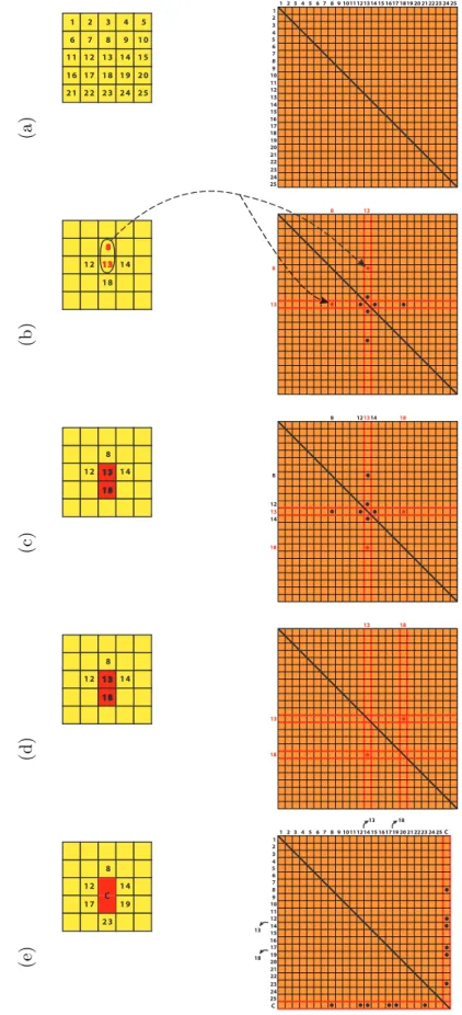
3.3 Illustration of one iteration in clustering process: (a) build the dis-similarity matrix; (b) compute the dissimilarities between neighbors; (c) locate the minimum dissimilarity; (d) merge the voxels and shrink

the matrix; (e) compute and add new dissimilarities. . . 80 3.4 Chessboard image sequence with 50 by 50 voxels and only two

clusters: (a) the red one and the black one; (b,c,e,f) the image at

t = 1, t = 10, t = 20 and t = 50 among 100 times; (d) the straight

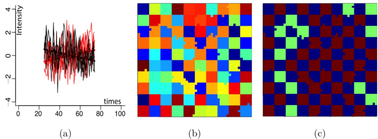
lines are the true TCs for two clusters and the noisy ones are the observations randomly picked from the sequence. . . 81 3.5 Local and global segmentation of Chessboard image sequence: (a)

the selection of number of local clusters: the red curve is the the control function in term of iteration and the green is the dissimilarity function during local clustering; (b) the color map of 100 local clusters from local clustering; (c) the averaged (estimated) TCs of local clusters in (b); (d) selection of number of global clusters: the purple curve, additional to (a), is the dissimilarity function during global clustering. (e) the color map of 2 global clusters from global clustering; (f) the average (estimated) TCs of global clusters. . . . 82 3.6 Local and global segmentation of shrunken Chessboard image

se-quence: (a) the shrunken true and observed observed TCs; (b) local clustering of shrunken chessboard with 2 clusters: the color map of 89 local clusters from local clustering; (c) global clustering of shrunken chessboard with 2 global clusters: the color map of 3 global clusters from global clustering. . . 83 4.1 Synthetic DCE image sequence: (left) The ground-truth

segmenta-tion of X ; (right) The true enhancement curves, ix_{(t), associated to}

LIST OF FIGURES 13 4.2 Two DCE-MRI image sequences on female pelvis with ovarian tumors

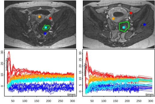
- each column shows one sequence. Up: image obtained at time t30 (after arterial phase) with the tumor ROI (green) together with four 4x4 squared neighborhoods (red, cyan, orange and blue), the red ones covering the iliac artery identified by the radiologist. Bottom (with corresponding colors): the sets of 16 time enhancement curves,

Ix(t

j), observed in the four squares after variance stabilization using

a= 0.45. . . 87

4.3 Synthetic image sequence segmentation using DCE-HiSET when δ varies: (Left) Fowlkes-Mallows Index (black stars) and its weighted version (red crosses) - (Right) number of clusters. Result with best indexes is achieved at δ = 0.6 (green dashed line). . . 92 4.4 Segmentation results of DCE-HiSET of synthetic image sequence

with δ equals to 0.5 (left), δ∗ _{= 0.6 (middle) and 2.0 (right) when}

α= 0.001. . . 92

4.5 FM index (left) and weighted FM index (right) when true enhance-ment curves, ix(t) (Fig. 4.1), are multiplied by 1 (solid), 2/3 (dashed)

and 4/3 (dotted). . . 93 4.6 Error maps when the SNR decreases by multiplying the true

en-hancements by 4/3 (left), 1 (middle) and 2/3 (right). . . 93 4.7 Competitors’ best results on synthetic sequence. Top: Best result of

k-means among 250 runs given the true number of clusters k = 11

(left); with highest FM index (middle) and with highest wFM index (right). Bottom: Results of HMRF-FCM, initialized by the result of

k-means with k = 11 and using ε = 0.2 (left), ε = 0.5 (middle) and ε= 2 (right). . . 95

4.8 Competitors’ best results on synthetic sequence. Left: MS (bwt,rts)=(0.06,11).

4.9 Error maps on synthetic sequence. From left to right, (Top) k-means with highest FM, HMRF-FCM with the highest FM, k-means with highest wFM, HMRF-FCM with highest wFM, (Bottom) best (FM-and wFM) results for MS, MS-NC, SLIC-NC (FM-and DCE-HiSET. . . 96 4.10 Segmentation results (the first two rows) and error maps (the last

two rows) of six methods when the true enhancements are multiplied by 1/2. The result with highest FM index is given for each method except HiSET. The right number of clusters is given for k-means and HMRFFCM. For HiSET, δ = 1 and α = 0.001. . . 100 4.11 Segmentation results (the first two rows) and error maps (the last

two rows) of six methods when the true enhancements are multiplied by 2/3. The result with highest FM index is given for each method except HiSET. The right number of clusters is given for k-means and HMRFFCM. For HiSET, δ = 1 and α = 0.001. . . 101 4.12 Segmentation results (the first two rows) and error maps (the last

two rows) of six methods when the true enhancements are multiplied by 4/3. The result with highest FM index is given for each method except HiSET. The right number of clusters is given for k-means and HMRFFCM. For HiSET, δ = 1 and α = 0.001. . . 102 4.13 Segmentation results (the first two rows) and error maps (the last

two rows) of six methods when the true enhancements are multiplied by 5/3. The result with highest FM index is given for each method except HiSET. The right number of clusters is given for k-means and HMRFFCM. For HiSET, δ = 1 and α = 0.001. . . 103 4.14 Segmentation results (the first two rows) and error maps (the last

two rows) of six methods when the true enhancements are multiplied by 2. The result with highest FM index is given for each method except HiSET. The right number of clusters is given for k-means and HMRFFCM. For HiSET, δ = 1 and α = 0.001. . . 104

LIST OF FIGURES 15 4.15 FM index (left) and weighted FM index (right) of best result of each

method when true enhancement curves are multiplied by ratios from 1/2 to 7/3. Only four methods (MS, MSNC, SLICNC and HiSET) are shown for FM and all methods are shown for weighted FM index.105 4.16 Number of clusters when α and δ vary for (left) local and (right)

global steps. . . 105 4.17 Normalized residual distributions (with δ=1/2/3/4/5, one color

for each) and normal distribution density (black and dashed) with

a=0.5/0.45/0.4 of variance stabilization. . . 105

4.18 Segmentation results of the two real DCE-MR image sequences using

δ= 3. . . 106

4.19 Squared zoom for the DCE-MR image sequence with δ equals 2 (left), 3 (middle) and 4 (right). Manually segmented ROI appears in black and clusters inside are numbered. The first sequence shows from 9 to 6 clusters (top). The second from 18 to 6 (bottom). . . . 106 4.20 Average TCs (after variance stabilisation) of the clusters inside the

manually segmented ROIs (see Fig. 4.19) with δ=2, 3 and 4 from left to right. Size of the corresponding clusters are given at the top of each subfigure with corresponding colors. . . 107

5.1 The improvement of SNR induced by HiSET. Left: Enhancement TCs of three randomly selected voxels. Right: Average enhancement TCs of clusters, to which the voxels belong, segmented by HiSET. . 113

5.2 Average enhancement TCs of clusters segmented by HiSET in a DCE image sequence. (a) ones of clusters in the entire DCE image sequence; (b) ones of clusters intersecting with manual ROI; (c) ones remained after filtration. Colors are assigned to clusters according to the AUC of the corresponding average TC. Red relates to the large AUCs and blue to the low ones. k stands for the total number of clusters. The size of each cluster (scaled by the size of image) is given as the length of its color bar on the color scale on the right. . 113

5.3 The filters remove from Figure 5.2 the average TCs showing (a) no enhancement, (b) negative enhancement, (c) arterial behavior, and (d) bumps or spikes, where (b) and (d) being due to motion artifacts. 114

5.4 The evolution of ROI during refinement process. From top to bottom: (a) manually delineated ROI by locating vertices of a polygon; (b) erosion of manual ROI by two voxels; (c) aggregate all clusters resulting from the segmentation by HiSET and intersecting eroded ROI; (d) a second erosion of previous ROI; (e) discard the small segments disconnected with the main one of previous ROI; (f) dilation of previous ROI to have final refined ROI. Left: binary mask of each ROI. Right: transparent mask of each ROI on color map of segmentation result. Colors are assigned to clusters according to the AUC of the corresponding average TC. Red relates to the large AUCs and blue to the low ones. . . 116

5.5 Filtration of average TCs within the refined ROI. Left: all average TCs; Right: filtered average TCs. Colors are consistent to Figure 5.2. k stands for the number of average TCs. The size of each cluster is given as the length of its color on the color bar on the right. . . . 117

LIST OF FIGURES 17 5.6 Qualitative features extracted from average TCs include (a)

max-imum enhancement (ME), enhancement amplitude (EA), and the slope angle during early and late phase made on one smoothed TC, and (b) Span/heterogeneity (SP) at the end of late phase based on the smoothed version (colored) of the average TCs (gray). . . 120 5.7 The results of auto-refinement of ROIs, for 6 DCE image sequence,

with various size. Each row shows the results for one DCE image sequence and its patient number is given at the beginning of the row. From left to right, (a) cropped binary masks of manual ROIs; (b) transparent masks on color maps of segmentation results of manual ROIs; (c) cropped binary masks of refined ROIs; (d) transparent masks on color maps of segmentation results of refined ROIs. Colors are assigned to clusters according to the AUC of the corresponding average TC. Red relates to the large AUCs and blue to the low ones. 124 5.8 Number of clusters resulted from manual ROI, manual ROI with

filtration of average TCs and refined ROI with filtration, in 17 DCE image sequences. . . 125 5.9 Binary classifications of ovarian tumor (potentially benign and

ma-lignant) based on two features: wmME and wmCA. From left to right, classification is based on (a) manual ROI, (b) manual ROI with filtration of average TCs and (c) refined ROI with filtration. From top to bottom, three classification method are used: k-means, LDA and SVM. Each type of tumor is represented with a shape, which is filled if the tumor is correctly classified (with ‘+’ in legend) by the model, otherwise (‘-’) is left unfilled. Decision area of each class is covered by dots in green for benign, blue for borderline and red for malignant. . . 127

5.10 Performance of binary classification of ovarian tumor (potentially benign and malignant), based on two features: wmME and wmCA. From left to right, three classification methods are used: (a) k-means, (b) LDA and (c) SVM. For each method, ROCs of both the classification (solid thinner line) and the leave-one-out cross-validation (dashed thicker line) are shown for three ROIs (black for manual ROI, red for manual ROI with filtration and green for refined ROI with filtration). Specially, for k-means, the ROC of the classification and the one of cross-validation are overlapped for each ROI. . . 128

5.11 Classifications of ovarian tumor with three classes (benign, borderline and malignant), based on two features: wmME and wmCA. From left to right, classification is based on (a) manual ROI, (b) manual ROI with filtration of average TCs and (c) refined ROI with filtration. Two classification methods are used: k-means (top) and SVM (bottom). Each type of tumor is represented with a shape, which is filled if the tumor is correctly classified (with ‘+’ in legend) by the model, otherwise (‘-’) is left unfilled. Decision area of each class is covered by dots in green for benign, blue for borderline and red for malignant. 129

5.12 The classification accuracy (ACC) in percentage. The classifications are based on (a) two features: wmME and wmCA; (b) three features: wmEA, wmCA and SP. Each group of bars corresponds to one of five classification models, including k-means with 2 classes, k-means with 3 classes, LDA with 2 classes, SVM with 2 classes and SVM with 3 classes. In each group, classifications are made individually on manual ROI, manual ROI with filtration of average TCs and refined ROI with filtration. . . 130

LIST OF FIGURES 19 6.1 Multi-view of two DCE volumes at portal phase: axial plane (left

column), coronal plane (middle column), sagittal plane (right col-umn). For both patients, sub-volumes are selected (surrounded by color frames in three plans) for further evaluation. . . 135

6.2 Multi-view of 3D DCE image sequence: axial plane (top row), coronal plane (middle row), sagittal plane (bottom row). From left to right, each column corresponds to a phase. . . 135

6.3 Residual densities after segmentations of different slices using the same sets of values of a and δ. Each column corresponds to one slice. The first row shows the segmentations based on a variance stabilization transform with a = 0.3 while the second with a = 0.25. For both values of a, two values of δ, 20 and 30, are used in HiSET. 136

6.4 For one slice given a = 0.3 and α = 0.001: (a) intensity-based seg-mentation using δl = δg = 20; (b) enhancement-based segmentation

based on average enhancement of clusters from last segmentation using δenh= 40; (c-d) intermediate segmentation using h = 0.5; (e-f)

intermediate segmentation using h = 1; (h-g) intermediate segmen-tation using h = 2. In (a-c,e,h), colors are arranged according to AUC of average intensity/enhancement curves from red (high AUC) to blue (low AUC), and the number of clusters in each segmentation is given on the left. In (d,f,g), same scatter is shown with every solid triangle standing for a cluster from intensity-based segmentation and ellipses highlight the cluster aggregations in intermediate segmentation.142

6.5 For one slice given a = 0.3 and α = 0.001: (a) intensity-based seg-mentation using δl= δg = 20; (b) enhancement-based segmentation

based on average enhancement of clusters from last segmentation using δenh = 40; (c-d) intermediate segmentation using h = 0.5; (e-f)

intermediate segmentation using h = 1; (h-g) intermediate segmen-tation using h = 2. In (a-c,e,h), colors are arranged according to AUC of average intensity/enhancement curves from red (high AUC) to blue (low AUC), and the number of clusters in each segmentation is given on the left. In (d,f,g), same scatter is shown with every solid triangle standing for a cluster from intensity-based segmentation and ellipses highlight the cluster aggregations in intermediate segmentation.143 6.6 DCE volume segmentation strategies. . . 144 6.7 Multi-view of 3D segmentations of three DCE volumes with a = 0.3

and α = 0.001. Left column: sub-volume #1, δl = 10, δg = 20, δ3D = 20 and δenh = 40; Middle column: sub-volume #3, δl = δg = 20,

δ3D = 20 and δenh = 40; Right column: sub-volume #2, δl = δg = 20

and δenh = 40. . . 144

6.8 The number of clusters in slices of which every cluster in volume consists, after volume segmentation of DCE volume #1 with a = 0.3,

α = 0.001, δl = 10, δg = 20, δ3D = 20 and different δenh for

enhancement clustering at the end. The width of box is proportional to the number of clusters in volume. . . 145 6.9 Effect of δl and δg: multi-view of 2D-to-3D segmentations of DCE

volume #1 with a = 0.3, α = 0.001, δ3D = 40 for volume seg-mentation based on intensity of slice segseg-mentation, δenh = 60 for

enhancement clustering at the end, and different δl and δg for slice

LIST OF FIGURES 21 6.10 Effect of δ3D: multi-view of 2D-to-3D segmentations of DCE volume

#1 with a = 0.3, α = 0.001, δl= 10, δg = 20 for slice segmentation,

δenh= 40 for enhancement clustering at the end, and different values

of δ3D. . . 147 6.11 Effect of δenh: multi-view of 2D-to-3D segmentations of DCE volume

#1 with a = 0.3, α = 0.001, δl = 10, δg = 20 for slice

segmenta-tion, δ3D = 20 for volume segmentation based on intensity of slice segmentation, and different values of δenh. . . 148

6.12 Multi-view of 2D-to-3D segmentations of DCE volume #1 with

a = 0.3 and α = 0.001. Top row: δl = 10, δg = 20, δ3D = 20 and

δenh = 40; Middle row: δl = δg = 20, δ3D = 30 and δenh = 50;

Bottom row: δl = δg = 30, δ3D = 40 and δenh = 60. . . 149

6.13 Multi-view of 2D-to-3D segmentations of DCE volume #3 with

a = 0.2 and α = 0.001. Top row: δl = 10, δg = δ3D = 20 and

δenh = 40; Middle row: δl = δg = 20, δ3D = 30 and δenh = 50;

Bottom row: δl = δg = 30, δ3D = 40 and δenh = 60. . . 150

6.14 Multi-view of direct 3D segmentation of DCE volume #2 with

a = 0.3 and α = 0.001. Top row: δl = 10, δg = δ3D = 20 and

δenh = 40; Middle row: δl = δg = 20, δ3D = 30 and δenh = 50;

List of Tables

4.1 The parameter information and the performance of all competitors and of DCE-HiSET. . . 94 4.2 FM index of the best result of each method given the true

enhance-ments are multiplied by different ratios. . . 98 4.3 Weighted FM index of the best result of each method given the true

enhancements are multiplied by different ratios. . . 98 5.1 Performance of classifications based on two features: wmME and

wmCA. . . 126 5.2 Performance of classifications based on three features: wmEA, wmCA

and SP. . . 126 6.1 Summary information of sub-volumes. . . 134

Chapter 1

Introduction

We start this introduction with a detailed context of cancer, perfusion imaging and their relationship, in order to help readers to understand the observations and the statistical challenge which was at the origin of this work. Then we introduce the statistical core of this thesis, which aims to address this challenge in a general framework and the several applications we have tackled using our development.

1.1 Medical context

1.1.1 Cancer

Being responsible to 8.2 million deaths and 14.1 million new cases all over the world in 2012 [Ferlay et al., 2013], cancer has been one of the most mortal and prevalent diseases in the world during decades. Several different factors such as the development of new therapeutic methodology and the improvement of detection and monitoring techniques for therapeutic follow-up provide strong hopes for cancer treatment. On one hand, more targeted and personalized therapeutic care with respect to patient’s states can significantly reduce the mortality. On the other hand, more advanced and comprehensive detection and monitoring tools might help provide earlier and more accurate diagnosis and detailed feedback about treatment used.

In this context, as an indispensable tool for radiologists to detect tumors and to monitor treatments, recent medical imaging tools, such as DCE-imaging, should pursue more standardized operation protocol as well as more robust analysis techniques, in order to more precisely and efficiently characterize the effect of therapies or drugs on tumors in clinical studies. With currently widely used imaging modalities, the development of medical imaging analysis techniques capable of exhibiting subtle functional information in an accurate and robust way plays one of the principle roles in the fight against cancer.

1.1.1.1 Treatments

In clinical practice, cancer can be treated by surgery, radiotherapy, chemotherapy, hormonal therapy, and targeted therapy. More recently, studies have shown that angiogenesis inhibitors controlling for example the VEGF has potential in treatment to many types of cancer, at least associated with other drugs.

Surgery

Surgery is an effective way to cure cancer showing localized tumors. However, once the cancer has metastasized to other sites of the body, a complete surgical removal is usually impossible since single metastatic tumorous cell can potentially grow into a new tumor. Unfortunately, localized tumors may be invasive cancer.

Radiotherapy

Radiation therapy consists in irradiating tumors with ionizing radiation to kill tumorous cells or at least stop their division by damaging their genetic material, and shrink tumors by stopping their growth. As surgery, radiation therapy works efficiently to localized tumors. Although in practice radiation therapy is provided in repeated small doses, such that most normal cells can recover from the effects of radiation, the damage to nearby healthy tissue can not be ignored. Moreover, radiotherapy is less effective when tumors are hypoxic because oxygen is an efficient radio-sensitizer.

1.1. MEDICAL CONTEXT 29

Chemotherapy

Chemotherapy consists in destroying tumorous cells with cytotoxic drugs and is typically applied along with radiotherapy or surgery when tumor metastasis has occurred. However, due to the complex characteristics of the tumorous vascular network (Figure 1.1), efficient targeting of the tumor with cytotoxic drugs could be a very difficult task. Most forms of chemotherapy target rapidly dividing cells and are not specific to tumorous cells. Therefore, chemotherapy might harm healthy tissue, especially tissues that have a high replacement rate. Moreover, during chemotherapy, patients can develop resistance to the cytotoxic drugs, which reduces the therapeutic effects.

Figure 1.1: Three tumors with their vascular structures: the left one illustrates a solid tumor with relatively simple vascular structure; the middle one illustrates a tumor growing from the left one due to tumorous angiogenesis, more capillaries and small vessels are formed during its growth; the right one illustrates an invasive tumor with an completely disorganized micro-vascular structure.

Hormonal therapy

Hormonal therapy consists in inhibiting the growth of certain types of tumorous cell by manipulating levels and activities of certain hormones. During the treatment, patients may suffer several side effects such as headache, nausea and tiredness, and increased risk of endometrial cancer, blood clots and stroke.

Targeted therapy

that can lead to cancers using agents targeting these pathways. Targeted therapy has to be adapted to issues such as patient’s state and type of tumors to be effective. However, researches show that cancer cells may become resistant to the drug.

Anti-angiogenic therapy

Angiogenesis is the process through which new blood vessels are generated from pre-existing ones [Birbrair et al., 2015]. In order to transform from a benign state to a malignant one, tumors need a dedicated blood supply to provide the oxygen and other essential nutrients they require. Therefore, tumors undergo an ‘angiogenic switch’ that breaks the balance between pro and anti-angiogenic factors in tumorous angiogenesis. Tumor vascular network is extended in a disorganized and inundant way.

From this perspective, anti-angiogenic therapy has been introduced in recent decades to regulate tumorous angiogenesis. It reduces the production of pro-angiogenic factors, prevent them binding to their receptors and block their actions. New therapeutic strategies have entered trials to combine anti-angiogenic inhibitor with chemotherapy to enhance delivery of cytotoxic molecules [Jain, 2005]. However, since many factors are involved in angiogenic phenomena, patients can develop resistance to anti-angiogenic therapy [Eikesdal and Kalluri, 2009]. With respect to these issues, indicators of tumorous vascular structure can play a significant role to personalized anti-angiogenic treatment to monitor their effects and to detect the development of drug resistance.

1.1.1.2 Detection and Monitoring

The choice of therapy depends upon the location, the grade of the tumor, the stage of the disease, as well as the general state of the patient. Meanwhile, each option has its specific targets, limitations and undesirable side effects. Therefore, for each individual, in order to avoid unnecessary burden brought by inefficient or even inappropriate therapy, critical decisions must be made based on both accurate

1.1. MEDICAL CONTEXT 31 information obtained at diagnosis and later during the monitoring of the treatment leading to a personalized treatment. In addition, pre-clinical studies (REMISCAN) which aim at improving the efficiency of a new drug also require accurate tumor characterization and monitoring techniques. These techniques are expected to be able to assess morphological, molecular or functional indicators, which are specific and predictive, of tumor state.

1.1.1.3 Indicators in cancer therapy

In order to help therapists and doctors in the personalization of the treatment, several tools are available.

Morphological

In clinical practice, morphological features of tumor, such as tumor size, have been considered to be indicators of the tumor’s therapeutic sensitivity [Stanley et al., 1977] and of the metastasis probability [Koscielny et al., 1984]. The RECIST criteria [Eisenhauer et al., 2009] is currently a clinical standard for the evaluation of cancer therapy, which classify tumors into three categories: stable, in regression or in progression. However, by definition, these criteria do not provide functional information on the tumor. For instance, according to this criteria, a tumor with a large necrotic core would be identified to be of equal risk as a highly vascularized tumor of the same size.

Molecular

Since certain specific molecules are produced along with the growth and func-tional modifications of tumors, monitoring the evolution of the concentration of those molecules can provide valuable information about the type and the stage of cancer [Ludwig and Weinstein, 2005]. Therefore, new technologies that can simul-taneously assess the concentration of thousands proteins has been developed and achieved a major improvement in diagnosis and tumor classification [Kulasingam and Diamandis, 2008].

Functional

As mentioned above, the assessment of tumor angiogenesis is able to reveal massive informations about functional modification of tumors. Quantification of the blood circulation inside tumorous vascular network became a proper indicator for cancer therapy. However, due to the complexity of tumorous vascular network during tumor growth (Figure 1.1), the blood circulation in the capillaries and small pe-ripheral vessels, which is defined as the micro-circulation, appear as the target to evaluate.

A common way to achieve this purpose is to visualize micro-vascular perfusion in order to characterize micro-vascular properties. The perfusion can be tracked by an imaging modality that measures the signal changes in the tissue of interest. The patterns of these changes are connected to the underlying perfusion. According to pathologists, tumorous tissue differs from normal tissue and usually shows heterogeneity, leading to similar variations in its micro-vascular properties. However, due to the growth of the tumor, one can expect the tumor to exhibit homogeneous sub-regions. Therefore, finding the sub-regions in tumorous tissue with similar perfusion patterns provides valuable information about tumor structure and its angiogenesis.

1.1.2 Perfusion Imaging

1.1.2.1 Technique

Among the new techniques, dynamic contrast enhanced (DCE) imaging using computed tomography (DCE-CT), magnetic resonance imaging (DCE-MRI) or ultrasonic imaging (DCE-US) is very promising, because it can non-invasively monitor the local changes in microcirculation secondary to the development of new vessels (neo-angiogenesis) induced by the growth of cancers. DCE imaging follows and analyzes the local distribution of a contrast agent in the blood circulation system after intravenous injection, using a sequential acquisition [Ingrisch and

1.1. MEDICAL CONTEXT 33 Sourbron, 2013]. The imaging modalities (CT, MRI and US) allow to have a 2D or 3D vision of a volume of the body during the acquisition. The DCE images taken at the same cross-section of patient during the entire acquisition period compose a

DCE image sequence. Since each image in DCE image sequence has a thickness,

every pixel in image has a volume. Therefore, DCE image consists of voxels instead of pixels as in general image.

1.1.2.2 Modalities Computed Tomography

The CT scanner is a device that measures the absorption by the tissues of X-rays emitted by a ray tube that rotates around the patient providing a Radon transform of the image [Herman, 2009]. After inversion of the Radon transform that is specific to each brand of device, it is possible to have a 2D or 3D vision reconstruction of a patient. The scanner allows to observe all areas of the body and all types of tissues (organs, bone, blood vessels, etc.).

Magnetic Resonance Imaging

With respect to CT, MRI is a less invasive tool based on the principle of nuclear magnetic resonance and uses some properties of atomic nuclei when exposed to magnetic fields. This tool is mainly dedicated to the imaging of the central nervous system, muscles, heart and tumors, it can observe the “soft” tissues with higher contrast than the scanner. Nevertheless, the CT scanner is not yet possible to be completely replaced by the MRI since some tissues such as bones are not observable with MRI, and moreover MRI does not allow precise localization at high time frequency, which indeed is needed for following the injection of a contrast agent bolus.

Ultrasonic imaging

Ultrasonic imaging uses high frequency sound waves that are reflected by tissue to produce images. Ultrasonic imaging is a non-invasive modality, which can be

brought directly and quickly to the patient in real time with a relatively low cost. However, it may provide less anatomical detail than CT and MRI. Moreover, it performs very poorly when there is a gas between the transducer and the organ of interest [Iftimia et al., 2011], due to the extreme differences in acoustic impedance.

1.1.2.3 Protocol

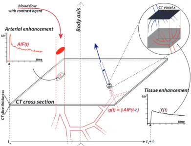
A contrast agent intravenously injected following the blood circulation is sketched in Figure 1.2, which illustrates the sequential image acquisition. The imaging acquisition starts before the injection in order to measure the pre-injection baseline consisting of non-uniform gray levels across the image without enhancement induced by contrast agent. The contrast agent is then sequentially followed during and after injection to monitor the kinetic of the vessel and tissue enhancements over time. The contrast agent arrives with the oxygenated blood through the aorta and main arteries. Its concentration within unit volume voxels is measured for the first time when it passes through the cross-section of the image. This measured concentration within a unit volume voxel inside the aorta is called the arterial input function (AIF). Afterwards, the contrast agent is distributed within the arterial system to enter the microvascular network made of capillaries within the tissues. The exchange within the tissue of oxygen, nutriments (such as glucose), and wastes (such as CO2) as well as contrast agent occurs at the microvascular level, and the concentration of contrast agent during this exchange is measured in all tissue voxels inside the image cross-section. Later, the contrast agent returns to the venous system with the deoxygenated blood. Each type of normal and pathological tissue has its own and specific microvascular architecture and physiology, leading to specific functional behavior, and therefore different temporal enhancement behavior after contrast injection.

This course of contrast agent is monitored by CT, MRI or US, which allows observations and therefore analysis at the voxel level at the same voxel grid for every image in the sequence. At each voxel of the image sequence, it provides a

1.1. MEDICAL CONTEXT 35

Blood flow with contrast agent

CT slic e thick ness Bo dy axis CT cross section 0 50 100 150 200 250 300 0 100 200 300 400 500 600 Arterial enhancement time UH 0 50 100 150 200 250 300 0 100 200 300 400 500 600 Tissue enhancement time UH CT voxel x AIF(t) g(t) = βAIF(t-δ) t_{* t*+} δ Y(t)

Figure 1.2: DCE-imaging and contrast agent circulation. The patient’s body is materialized by the mixed arrow.

injection) and the varying effect of the contrast agent related to its concentration (after the injection). Removing the pre-injection phase and subtracting the baseline from the time-intensity curve, we can construct a time enhancement curve (TEC) only for the enhancement induced by contrast agent during the the post-injection phase. In Figure 1.2, the red curve represents the TEC for a voxel in the aorta, and the black curve represents TEC for a voxel in the tissue of interest such as tumor. Two types of curves reveal different characteristics of tissues and both are of interest of further analysis. In the sequel, without more precision, time curve (TC) will refer either to TIC or TEC, depending on the study purpose.

1.1.2.4 Perfusion analysis

The TCs from the DCE image sequences can be analyzed using qualitative or quantitative approaches. In qualitative analysis, descriptive features such as maximum enhancement (ME), area under the curve (AUC) and time to peak (TTP) are directly derived from the observed TCs of voxels. These measures are used either individually [Tuncbilek et al., 2005; Medved et al., 2004; Tuncbilek et al., 2004] or as a combination [Lavini et al., 2006]. However, they are not

normalized and are sensitive to the variations of patient’s physiology (stress, blood pressure, heartbeat, etc.) and the acquisition protocols such as the number of images in the sequence, the amount of injected contrast agent, and the total acquisition duration. In quantitative analysis, pharmacokinetic models such as standard and extended Tofts [Tofts et al., 1995; Tofts, 1997] and Brix models [Brix and et al., 2004] and blood flow models [Axel, 1980; Fieselmann et al., 2011; Ostergaard et al., 1996] are commonly used in order to remove dependencies existing in qualitative analysis. These models describe the diffusion of contrast agent from blood plasma into the extracellular extravascular space (EES) using different assumptions and simplifications. Well-defined physiological parameters, such as tissue blood flow, blood volume and vessel permeability, are extracted by the deconvolution of the tissue response to the patient’s AIF, through 1) parametric estimation in pharmacokinetic models [Brochot et al., 2006], 2) semi-parametric techniques based on adaptive smoothing of each observed TC [Schmid et al., 2009] and 3) non-parametric estimation based on Laplace deconvolution in the blood flow model [Comte et al., 2014].

1.2 Issues in DCE imaging

1.2.1 Issues for analysis of DCE image sequences

DCE imaging, however, suffers from several issues, which hamper its large diffusion. First of all, consensus is lacking for the analysis strategy. Secondly, voluntary and involuntary movements (such as breathing and cardiac motion, and non-periodic motions such as bowel peristalsis) limit the quality of the analysis, and can be addressed by motion correction methods [Glocker et al., 2011; Sotiras et al., 2009]. Finally, low SNR is a common issue in dynamic in vivo imaging due to the short time allowed to record the signal within the image sequence and affects any quantitative estimation1_{. For CT, because of the need to minimize the tissue irradiation during}

1.2. ISSUES IN DCE IMAGING 37 the entire sequence, using low Kvs and MAs to reduce the total X ray dose leads to very poor quality for individual images. For MRI, high-speed sequences are obtained with a high cost in signal. The larger resolution we want without changing magnetic field, fewer protons arrive at the each voxel, therefore, the lower SNR is.

1.2.2 SNR improvement via segmentation

To improve SNR when analyzing DCE images, either large manual regions of interest (ROI) are drawn by the radiologist or image sequence is denoised by spatial filtering techniques. However, large ROI could end up with a lack of homogeneity by mixing different types of TCs, and, filtering techniques could trigger a tricky balance between information and noise when the TC shows variation of high frequency and induce a low spatial resolution. This work focus on this last issue.

DCE image sequence reveals tissues (organs, tumors, metastasis, vessels, bones, muscles, fat, etc.) having homogeneous properties that can be considered from an image processing point-of-view as objects in a scene. Consequently, one can think to recover these tissues/objects. It leads to segment the DCE image sequence into regions (of voxels) showing homogeneous TCs. This provides the opportunity to improve SNR without loss of spatial and temporal information, by averaging the TCs in these recovered regions. This alternative is known as DCE image sequence

segmentation. In this context, DCE image sequence is considered as a spatial (2D

or 3D) domain made of voxels. At each voxel, one can observe a TC in time domain. Hence, one needs a double representation of both spatial structure (voxel) and time structure (curve). Segmentation in this context is to obtain a partition of the spatial domain into subsets having their time structure homogeneous.

Depending on the plain positions of the DCE image sequences, the amount of tissues could potentially vary from only a few to many. These tissues could be filled, surrounded or interrupted by air, water or pure geometry effects (e.g. colon) but also appear at several disconnected locations in the image. Therefore, DCE image segmentation should have the ability in presence of noise to recover an

unknown number of homogeneous regions that could be numerous and spatially disconnected. Moreover, DCE image segmentation should take advantage of functional information embedded in the image sequence in order to preserve as much as possible the temporal information. From a statistical point-of-view, this is ensured by the use of adaptive methods (in time domain). However, let us point out that, as the functional information results from the convolution with the AIF, one can expect the signals to be smooth enough in Hölder spaces.

1.3 Statistical core of this PhD thesis

We present the statistical core of this PhD thesis in a general context. In this work, we propose a new method, called Hierarchical Segmentation using Equivalence Test

(HiSET), aiming to cluster functional (e.g. with respect to time) features or signals

discretely observed with noise on a finite metric space considered to be a landscape and where the noise on the observations is assumed independent Gaussian with known constant variance. HiSET employs a multiple equivalence test derived from a multi-resolution comparison test in the time domain, which is known to be adaptive to the unknown Hölder regularity of signal, in order to compare two elements in the landscape. Considering the p-value of the multiple equivalence test as dissimilarity measure, HiSET is a bottom-up hierarchical clustering algorithm consisting of two steps: one local and one global.

In the local step (region growing), starting from a partition made of all elements

of the metric space, only spatial neighbors may be aggregated into larger clusters. One can view the resulting partition of this local step as the collection of spatially adaptive super-elements.

In the global step (region merging), starting from the partition resulting from the

local step, all clusters may be aggregated into larger clusters, regardless of their disconnectedness.

1.4. MEDICAL APPLICATIONS 39 homogeneity discrepancy between two functional features and α the significance level (upper bound of the Type I error) of the multiple equivalence test, which controls the probability to stop too late in the iterative process. Given α and

δ, both steps stop automatically through a proper control of the Type I error,

providing an adaptive choice of the number of clusters. Homogeneity discrepancy is ensured as parameter δ controls whether the difference of two functional features is close to 0 or not, regardless any modeling of these features. In this spirit, it is a human interpretable parameter as it is meaningful on noiseless observations.

For a set made of functionally piecewise homogenous subsets, HiSET is proven to be able to retrieve the true partition with high probability when the number of observation times is large enough.

In the application for DCE image sequence, the assumption is achieved by the modeling of the observed intensity in the sequence through a proper variance stabilization, which depends only on one additional parameter a. Combing this DCE imaging modeling step with our statistical core, HiSET, provides DCE-HiSET.

1.4 Medical applications

1.4.1 2D and 3D segmentation

We have applied DCE-HiSET on both 2D and 3D DCE image sequence segmentation. For 3D sequences, we have considered two strategies, a 2D-to-3D strategy and a direct 3D strategy. The 2D-to-3D strategy aims to propagate 2D-regions obtained from a first 2D-segmentation of each slice by doing the complete 3D-segmentation starting from the partition made of all 2D-partitions. The direct 3D strategy applies DCE-HiSET directly considering neighbors in the 6 directions (4 in the slice plus 2 to go from slice to slice).

1.4.2 ROI refinement and tumor classification

We also used DCE-HiSET as a preprocessing step to refine a roughly manually delineated ROI made by cliniciens. Followed by a series of erosion-dilation process, DCE-HiSET helps remove the regions only located at or connected to the border of the manual ROI while preserving the homogeneous regions connected to the interior of the ROI. We apply the result of this refinement to a series of DCE image sequences of 99 ovarian tumors graded with respect to their aggressiveness according to the biology from a biopsy. Using several classification models covering unsupervised and supervised approaches, we show that the classification with respect to their grade of these ovarian tumors based on the functional features observed in the ROI was improved after ROI refinement.

1.5 Reading guide

In Chapter 2, we review the existing clustering methods that have been applied to DCE image sequence segmentation. In Chapter 3, we describe the statistical model (§3.1), the multiple equivalence test (§3.2) and the two-step clustering procedure with its theoretical properties (§3.3). In Chapter 4, we apply and evaluate the proposed method on 2D DCE image sequence. We compare the proposed method to other state-of-the-art methods with synthetic DCE image sequence and study the parameter influence on the segmentation result with real DCE image sequences, along with the model verification. Additionally, in Chapter 5, an automatic strategy aiming to refine the manual ROI is described with an evaluation of robustness and efficiency. In Chapter 6, we evaluate the proposed method on 3D DCE image sequence. We explore and evaluate several segmentation strategies based on the proposed method. This work being supported by a CIFRE contract in the company Intrasense, Chapter 7 is devoted to present shortly the company, its medical imaging software Myrian®, together with how this work has been implemented in Myrian® and how the company may benefit from this implementation.

Chapter 2

Previous state of the art

2.1 Previous works related to DCE image sequence

segmentation

Region (object)-based segmentation has been investigated for detecting lesions [Agner et al., 2013; Chen et al., 2006; Irving et al., 2016; McClymont et al., 2014; Shi et al., 2009; Shou et al., 2016; Stoutjesdijk et al., 2012; Tartare et al., 2014], or for retrieving internal structure of organs using a prior knowledge on the number of tissue in the organ of interest [Abdelmunim et al., 2008; Chevaillier et al., 2011; Lecoeur et al., 2009; Li et al., 2012a]. With respect to the requirement of training dataset, we divide all classification methods, which have been used in these works to classify voxels into classes (regions), into two categories: supervised and unsupervised. Supervised approaches require training dataset to build the classifiers that are used to classify new dataset. Unsupervised approaches do not require training dataset and are referred in this work as clustering-based image segmentation methods. Supervised approaches are usually used in conjunction with unsupervised approaches to achieve a more specific objective.

2.1.1 One-stage unsupervised approaches

Chen et al. [2006] used a fuzzy c-means (FCM) clustering to segment a predefined breast ROI into two classes: lesion and non-lesion. In this work, DCE image sequence has six acquisition times: one for pre-contrast and five for post-contrast. FCM takes enhancements at post-contrast times as input. After FCM, the soft membership map is binarized (two classes) with a empirically chosen threshold. And hole filling is needed to get a closed lesion.

Shi et al. [2009] also used FCM with two classes to segment suspicious breast lesion. After the hole filling operation to remove isolated voxels within lesion region, the level-set (LS) method was used to refine the boundary of lesion. In this work, each sequence has 10 images: one for pre-contrast and 9 for post-contrast, but only the standard deviation and maximum enhancement computed for every voxel are used for FCM.

Lecoeur et al. [2009] investigated the segmentation of lesion and internal struc-ture in brain for multimodal (multi-channel as RGB) imaging, which is very similar to DCE imaging in the sense of image sequence. This work introduced a hierar-chical segmentation method that iteratively uses graph cut (GC) to separate two classes/tissues (object and background), until expected number of classes/tissues are segmented. The energy function to be minimized in GC contains region in-formation and border inin-formation. For region inin-formation, each class is modelled by a multivariate (univariate for each channel) Gaussian distribution. Border information is provided by the spectral gradient.

Chevaillier et al. [2011] proposed a two step method for the segmentation of internal structure (compartments) in kidney. In the first step, it constructs a graph structure with automatically determined number of nodes from all voxels, using a growing neural gas algorithm. In the second step, it merges the nodes into three classes using two thresholds of qualitative parameters based on time curves, which have 256 acquisition times.

2.1. PREVIOUS WORKS RELATED TO DCE IMAGE SEQUENCE SEGMENTATION43 with k equal to 5. Wavelet coefficients were selected by hard thresholding with

minimizing Stein’s unbiased risk. It used cosine distance of selected wavelet coefficient as distance for k-means.

Shou et al. [2016] developed soft null hypotheses in testing procedure to classify (identify) brain lesion voxels with enhancement out of other voxels without, leading to a binary classification: lesion and non-lesion. Several null hypotheses were proposed to quantify the qualitative behavior of time series. PCA was used to reduce the dimension. The third and fourth principle components (PCs) are considered as the representative of enhancement and are further used in testing. In this work, soft null hypotheses were compared to the clustering based on a mixture of k normal distributions with k varying. This work also proposed two points to argue the failure of clustering: there is a continuous change in intensity from non enhancement to strong enhancement, and lesion only accounts for a small portion of voxels that do not have high influence on the estimation of the parameters for mixture distributions.

For breast lesion segmentation, Agner et al. [2013] proposed to use a spectral embedding (SE) to represent time intensity curves with only 3 dimensions in order to have a stronger gradient and to provide more descriptive region statistics for active contour (AC) model, which is later used to define the boundary of lesion. Regional information is modelled by a mixture of two multivariate Gaussian distributions, one for lesion and the other for non-lesion. In this work, the proposed method, SE-AC, was compared to FCM-AC that uses FCM in conjunction with AC model. Tartare et al. [2014] used spectral clustering to partition a ROI on prostate into clusters. Considering a k-nearest neighbor graph, the computed affinity matrix incorporates the spatial information of image. The number of clusters equals to the number of eigenvectors used in spectral representation of time curves and is automatically estimated using a normalized modularity criterion. With this number, voxels are clustered using k-means. Additionally, clusters were labelled by comparing the averaged curves to AIF.

clustering and GC for breast lesion detection and delineation. MS clustering is able to produce spatially contiguous regions by treating spatial coordinates as part of input along with feature domain and does not need a predefined number of clusters. After removing clusters corresponding to vessels and non-enhanced tissues, a region adjacent graph was constructed considering each remaining cluster as a vertex. GC was made to separate lesion from surroundings. Like some earlier works, DCE image sequence has only 4 or 5 acquisition times: one for pre-contrast and others for post-contrast. For each voxel, MS used a feature vector consisting of its spatial coordinate and its enhancement at post-contrast times. GC used a measure based on the mean enhancement during post-contrast.

2.1.2 Multi-stage approaches mixing unsupervised and

su-pervised methods

Stoutjesdijk et al. [2007, 2012] proposed a three-step strategy for the segmentation of lesion and subdivision in breast. Firstly, Otsu thresholding [Otsu, 1979] was applied on the first enhancement to delineate a lesion in breast. Secondly, mean shift (MS) clustering was used to subdivide the lesion into contiguous and homo-geneous clusters using enhancement parameters. Finally, classifiers such as linear discriminative analysis (LDA) and support vector machine (SVM) were trained on kinetic parameters to select the most malignant ROI.

Irving et al. [2014, 2016] used a supervoxel over-segmentation to retrieve local homogenous regions and a parts-based graphical model to include global anatomical relationships. To get supervoxels, an adapted k-means clustering method, simple linear iterative clustering (SLIC), was used on the data represented by PCA with the first three PCs. SLIC is based on a new distance combining the feature distance and spatial distance. The number of supervoxels and the compactness parameter are required to be defined. Then supervised classifier LDA was trained to assign one of three classes (tumor, bladder and lumen) to each supervoxel. Supervoxel connectivity was represented by a graph and belief propagation was used to identify

2.1. PREVIOUS WORKS RELATED TO DCE IMAGE SEQUENCE SEGMENTATION45 three nodes for three classes from all supervoxel candidates. In addition, these

works pointed out that supervoxels can be produced using methods including SLIC, MS, normalized cut (NC), etc.

2.1.3 Discussion

In summary, these works focused only on the partial segmentation for lesions and organs. However, the approaches that have been investigated in [McClymont et al., 2014; Irving et al., 2014, 2016] revealed a two-step framework that can be generalized to DCE image sequence segmentation, which, to remind, is a complete segmentation of the entire spatial domain in image. In this framework, the over-segmented supervoxels are generated using methods such as MS or SLIC in the first step, and then fully connected conditional random fields (CRF) or normalized cut (NC, multi-class version of GC for binary) propagates the supervoxels into a final partition of the entire spatial domain. In other words, the method according with this framework will also be a local-global method, as what we expected for our method. Hence, they appear to be excellent competitors.

2.2 Clustering methods for DCE image sequence

segmentation

In this section, we will first describe the issues of DCE image sequence segmentation. Then, considering that DCE image sequence segmentation is a special case of general image segmentation, we will broaden the survey of literature and review the clustering methods, mentioned in the works from Section 2.1, in the perspective of image segmentation. Roughly speaking, we divide these clustering methods into three categories and discuss about their limitations. Finally, among these methods, we will introduce the technical details, according to the original problem setting, about five of them, which will be compared to our method later in Section 4.2.

2.2.1 Issues of DCE image sequence segmentation

In this thesis, we focus only on unsupervised approach that does not require a training dataset. Clustering-based methods involved in previous works provide only a partial (or binary) segmentation of the DCE image sequence. Despite being potentially adaptable to our purpose (complete segmentation of the spatial domain), these methods have never been used for this objective to our knowledge. Moreover, we do not expect to have a prior knowledge on the number of regions since we want to deal with large images potentially covering several organs, tumors or metastasis that are known to be heterogeneous.

With respect to time structure representation in DCE image sequence, both parametric and non-parametric approaches have been investigated. Parametric representations use a fixed number of qualitative descriptors based on curves (slope, ME, AUC, etc), or, of eigenvectors resulting from a principle component analysis (PCA) [Irving et al., 2016; Shou et al., 2016] or from a spectral embedding [Agner et al., 2013; Tartare et al., 2014] for all the curves. By construction, these approaches can not be adaptive to the curve regularity that may change from voxel to voxel. Non-parametric representations such as wavelet coefficient [Li et al.,